Magnetization Degree of Gamma-Ray Burst Fireballs: Numerical Study

Abstract

The relative strength between forward and reverse shock emission in early gamma-ray burst afterglow reflects that of magnetic energy densities in the two shock regions. We numerically show that with the current standard treatment, the fireball magnetization is underestimated by up to two orders of magnitude. This discrepancy is especially large in the sub-relativistic reverse shock regime (i.e. the thin shell and intermediate regime) where most optical flashes were detected. We provide new analytic estimates of the reverse shock emission based on a better shock approximation, which well describe numerical results in the intermediate regime. We show that the reverse shock temperature at the onset of afterglow is constant, $(\bar{\Gamma}_{d}-1)\sim 8\times 10^{-2}$, when the dimensionless parameter $\xi_{0}$ is more than several. Our approach is applied to case studies of GRB 990123 and 090102, and we find that magnetic fields in the fireballs are even stronger than previously believed. However, these events are still likely to be due to a baryonic jet with $\sigma\sim 10^{-3}$ for GRB 990123 and $\sim 3\times 10^{-4}-3$ for GRB 090102.

1 INTRODUCTION

A widely accepted model for producing gamma-ray bursts (GRBs) is based on the dissipation of a relativistic outflow (e.g. Piran 2004; Zhang & Mészáros 2004). The internal energy produced by shocks is believed to be radiated via synchrotron emission. Although the presence of strong magnetic fields is crucial in the model, the origin and its role in the dynamics are still unknown. Understanding the nature of the relativistic outflow, especially the energy content, acceleration and collimation, is a major focus of international theoretical and observational efforts. Relativistic outflow from a GRB central engine is conventionally assumed to be a baryonic jet, producing synchrotron emission with tangled magnetic fields generated locally by instabilities in shocks (Medvedev & Loeb 1999; Nishikawa et al. 2005; Spitkovsky 2008). Recently an alternative magnetic model is attracting attention from researchers (e.g. Drenkhahn & Spruit 2002; Fan et al. 2004; Zhang & Kobayashi 2005; Lyutikov 2006; Giannios 2008; Mimica et al. 2009, 2010; Zhang & Pe’er 2009; Zhang & Yan 2011; Narayan et al. 2011; Granot 2012). The rotation of a black hole and an accretion disk might cause a helical outgoing Magnetohydrodynamic (MHD) wave which accelerates material frozen into the field lines (Tchekhovskoy et al. 2008; McKinney & Blandford 2009; Komissarov et al. 2009). In the magnetic model, a fireball is expected to be endowed with primordial magnetic fields from the central engine.

The first detection of ten percent polarization of an optical afterglow just 160 sec after the GRB explosion (Steele et al. 2009) opens the exciting possibility of directly measuring the magnetic properties of the GRB outflow. Recently polarization measurements of the prompt gamma-ray emission were also reported (Kalemci et al. 2007; McGlynn et al. 2007; Götz et al. 2009; Yonetoku et al. 2011). Although these polarization measurements suggest that at least some GRB outflows contain ordered magnetic fields and they are still baryonic, the sample is small and further observations will be necessary to confirm the magnetic model and/or to understand the role of magnetic fields in the dynamics. In this paper, we revisit the magnetization estimate of the GRB outflow (hereafter “fireball”) based on photometric observations of early optical afterglow. It is more sensitive to the magnetic energy density, rather than the length scale of magnetic fields in the fireball, and it is complementary to polarimetric methods (e.g. Lazzati 2006; Toma et al. 2009).

A steep decay in early optical afterglow light curves is usually considered as a signature of the reverse shock emission (e.g. Akerlof et al.1999; Sari & Piran 1999; Meszaros & Rees 1999; Soderberg & Ramirez-Ruiz 2002; Li et al. 2003; Fox et al. 2003; Nakar & Piran 2005). The early emission contains precious information on the original ejecta from the central engine. The magnetization of the fireball can be evaluated by using the relative strength of the forward and reverse shock emission (Fan et al. 2002, 2005; Zhang et al. 2003; Kumar & Panaitescu 2003; Gomboc et al. 2008). However, the standard method is obtained by using a simplified shock dynamics model, and Nakar & Piran (2004) have shown that the simple model is inaccurate in the intermediate regime between the thin and thick shell extremes. Since most observed events are in the intermediate regime, here we numerically re-examine the interplay between the forward and reverse shock emission at the onset of afterglow. In Section 2 we set out a simple conventional approach to understanding the two shock emissions and refine the definition of the magnetization parameter in Section 3. In Section 4 we consider a new approximation to discuss the reverse shock emission in the intermediate regime. In Section 5, we then test these analytic approximations with numerical simulations. In Section 6 we present case studies of GRB 990123 and 090102 in terms of the magnetization parameter. Finally in Section 7 we summarize the results.

2 Forward and Reverse Shock

We consider a homogeneous fireball of energy $E$ and a baryonic load of total mass $M$ confined initially in a sphere of radius $r_{0}$. We define the dimensionless entropy $\Gamma_{0}\equiv E/Mc^{2}\gg 1$. This fireball expands into a homogeneous interstellar medium (ISM) of particle density $n_{1}$. This can be considered to be a free expansion in its initial stage. After a short acceleration phase, the motion becomes highly relativistic, and a narrow shell is formed. After the fireball shell uses up all its internal energy, it coasts with a Lorentz factor of $\Gamma_{0}$ and the radial width $\Delta_{0}\sim r_{0}$.

The deceleration process of the shell is described with two shocks: a forward shock propagating into the ISM and a reverse shock propagating into the shell. The forward shock is always ultra relativistic, while the evolution of the reverse shock is determined by a dimensionless parameter $\xi_{0}=(l/\Delta_{0})^{1/2}\Gamma_{0}^{-4/3}$ where $l=(3E/4\pi m_{p}n_{1}c^{2})^{1/3}$ is the Sedov length and $m_{p}$ is the proton mass. If $\xi_{0}<1$ (so called thick shell case), the reverse shock becomes relativistic in the frame of the unshocked shell material and it drastically decelerates the shell. If $\xi_{0}>1$ (thin shell case), the reverse shock is inefficient at slowing down the shell. The deceleration radius $r_{d}$ and the Lorentz factor $\Gamma_{d}$ of the shocked material at $r_{d}$ are usually approximated as $r_{d}\sim l^{3/4}\Delta_{0}^{1/4}$ and $\Gamma_{d}\sim(l/\Delta_{0})^{3/8}$ for $\xi_{0}<1$, and $r_{d}\sim l/\Gamma_{0}^{2/3}$ and $\Gamma_{d}\sim\Gamma_{0}$ for $\xi_{0}>1$ (Sari and Piran 1995; Kobayashi et al. 1999). After the deceleration, the profile of the shocked ISM medium begins to approach the Blandford & McKee (1977) solution.

We first discuss the forward and reverse shock emission by using these conventional estimates, and the accuracy (i.e. correction factors) will be numerically examined later. The deceleration of a shell happens at an observer time

$$t_{d}=C_{t}\frac{l}{c\Gamma_{0}^{8/3}},$$ (1)

where $C_{t}\sim(\Gamma_{d}/\Gamma_{0})^{-8/3}\sim\max(1,\xi_{0}^{-2})$ and all the correction factors in this paper, including $C_{t}$, are defined as ones relative to the conventional thin shell estimates. At the deceleration time, the forward and reverse shock regions have almost the same Lorentz factor and internal energy density. However, the reverse shock region has a much larger mass density and therefore it has a lower temperature. Introducing a magnetization parameter $R_{B}\equiv\epsilon_{B,r}/\epsilon_{B,f}$, it is shown that the typical frequencies $\nu_{m}$ and peak fluxes $F_{\nu,max}$ of the synchrotron emissions from the two shocks are related as (Kobayashi & Zhang 2003; Zhang et al. 2003)

$$\frac{\nu_{m,r}(t_{d})}{\nu_{m,f}(t_{d})}=C_{m}\Gamma_{0}^{-2}R_{B}^{1/2},\ \ \ \ \frac{F_{\nu,max,r}(t_{d})}{F_{\nu,max,f}}=C_{F}\Gamma_{0}R_{B}^{1/2},$$ (2)

where $C_{m}\sim(\Gamma_{d}/\Gamma_{0})^{-4}\sim\max(1,\xi_{0}^{-3})$ and $C_{F}\sim(\Gamma_{d}/\Gamma_{0})^{2}\sim\min(1,\xi_{0}^{3/2})$ are correction factors, the subscripts $r$ and $f$ indicate reverse and forward shock, respectively. We have assumed that the electron equipartition parameter $\epsilon_{e}$ and the electron power-law index $p$ are the same for the two shock regions, but with different magnetic equipartition parameter $\epsilon_{B}$ as parametrized by $R_{B}$. The reason we introduce the $R_{B}$ parameter is that the fireball might be endowed with primordial magnetic fields from the central engine. We can give a simple relation $\nu_{c,r}/\nu_{c,f}\sim R_{B}^{-3/2}$ between the cooling break frequencies of the two shock emissions (Zhang et al. 2003). As we will see in the next section, this simple estimate is good enough for the magnetization estimate.

3 Magnetization Estimates

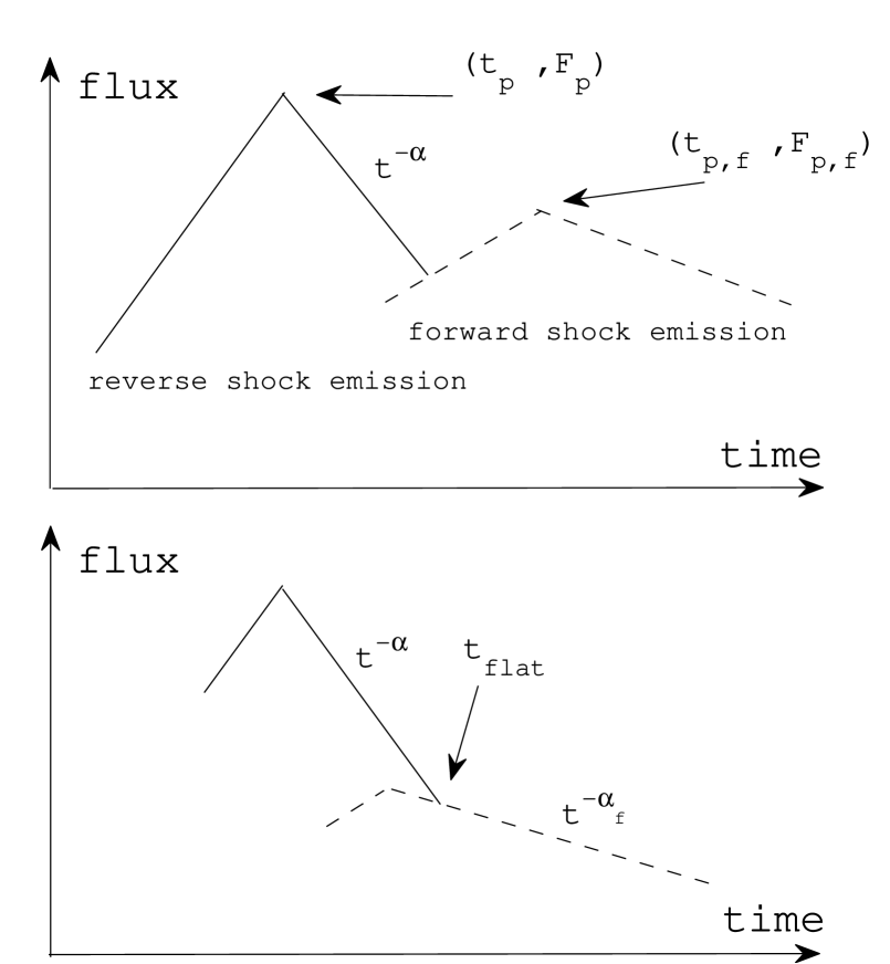
Figure 1: Early steep decay: optical afterglow, produced as a composition of the reverse shock emission (solid line) and forward shock emission (dashed line). Two peaks (top panel) and a flattening (bottom panel) in the light curve.

For no or moderate primordial magnetic fields in a fireball , we expect $\nu_{m,r}\ll\nu_{m,f}$ and $\nu_{c,r}\lower 2.15277pt\hbox{$\;\buildrel<\over{\sim}\;$}\nu_{c,f}$ at the peak time of the reverse shock emission $t_{p}\sim t_{d}$. The optical band $\nu_{opt}$ should satisfy a relation $\nu_{m,r}<\nu_{opt}<\nu_{c,r}$ during the early steep decay phase of the reverse shock emission. Otherwise the decay is much slower or faster than the typical decay $t^{-2}$ (Kobayashi 2000). There are four possible relations between the break frequencies and the optical band at the peak time $t_{p}$: (a) $\nu_{m,r}<\nu_{opt}<\nu_{m,f}<\nu_{c,r}<\nu_{c,f}$, (b) $\nu_{m,r}<\nu_{opt}<\nu_{c,r}<\nu_{m,f}<\nu_{c,f}$, (c) $\nu_{m,r}<\nu_{opt}<\nu_{c,r}<\nu_{c,f}<\nu_{m,f}$, and (d) $\nu_{m,r}<\nu_{m,f}<\nu_{opt}<\nu_{c,r}<\nu_{c,f}$. In the cases (a) and (b), the forward shock emission peaks at $t_{p,f}$ when the typical frequency $\nu_{m,f}$ goes through the optical band (the top panel in figure 1). Using $\nu_{m,f}\propto t^{-3/2}$, we get the peak time and peak flux ratio

$$R_{t} \equiv t_{p,f}/t_{p}=\left(\nu_{m,f}(t_{p})/\nu_{opt}\right)^{2/3},$$ (3)

$$R_{F} \equiv F_{p}/F_{p,f}=(F_{\nu,max,r}(t_{p})/F_{\nu,max,f})(\nu_{opt}/\nu_{m,r}(t_{p}))^{-(p-1)/2}$$ (4)

where $F_{p}$ and $F_{p,f}$ are optical peaks in the time domain, while $F_{\nu,max,r}$ and $F_{\nu,max,f}$ are peaks in the spectral domain for a given time. The hydrodynamics evolution of a reverse shocked shell is investigated in Kobayashi & Sari (2000), and the decay index $\alpha\sim(3p+1)/4\sim 2$ of the reverse shock emission is found to be almost independent of $\xi_{0}$ when $\nu_{m,r}<\nu_{opt}<\nu_{c,r}$. Combining Equations (2), (3) and (4), we obtain (Gomboc et al. 2008)

$$R_{B}=\left(\frac{R_{F}^{3}\Gamma_{0}^{4\alpha-7}}{C_{F}^{3}C_{m}^{2(\alpha-1)}R_{t}^{3(\alpha-1)}}\right)^{2/(2\alpha+1)}\sim\left(\frac{R_{F}^{3}\Gamma_{0}}{C_{F}^{3}C_{m}^{2}R_{t}^{3}}\right)^{2/5}.$$ (5)

At this stage, we assume that $\Gamma_{0}$ is a known quantity, and we will discuss how to estimate $\Gamma_{0}$ from early afterglow observations in section 5.3. In the case (c), if the forward shock emission makes a transition from the fast cooling to the slow cooling regime before it peaks, it becomes equivalent to the case (b). The estimate (5) is valid. On the other hand, if it is still in the fast cooling regime when $\nu_{c,f}$ crosses the optical band, the forward shock emission rises and decays very slowly as $t^{1/6}$ and $t^{-1/4}$ (Sari et al. 1998). Since this behavior is not consistent with most early afterglows, we do not discuss the details . Finally, in the case (d), the forward shock emission also peaks at the onset of afterglow, and it follows that $R_{t}=1$. It is possible to show that Equation (5) is still valid.

When an early afterglow light curve shows a flattening at $t=t_{flat}$ after the steep decay phase (the bottom panel in figure 1), the reverse shock emission dominates at early times. The forward shock peak is masked by the reverse shock emission, the peak ($t_{p,f}$, $F_{p,f}$) is not observationally determined. In such a case, the upper limit $t_{p,f}=t_{flat}$ gives a rough estimate of $R_{B}$. Considering that the reverse and forward shock emission components are comparable at the flattening, we obtain $R_{F}\sim R_{t}^{\alpha}$. Substituting this relation into Equation (5), we get

$$R_{B}\sim\left(\frac{R_{t}^{3}\Gamma_{0}^{4\alpha-7}}{C_{F}^{3}C_{m}^{2(\alpha-1)}}\right)^{2/(2\alpha+1)}\sim\left(\frac{R_{t}^{3}\Gamma_{0}}{C_{F}^{3}C_{m}^{2}}\right)^{2/5}.$$ (6)

where $R_{t}=t_{flat}/t_{p}$. If the forward shock emission peaks earlier $t_{p,f}<t_{flat}$, the real value of $R_{B}$ might be slightly different. To evaluate how $R_{B}$ depends on $t_{p,f}$, we refer to the scalings $R_{t}\propto t_{p,f}$ and $R_{F}\propto t_{p,f}^{\alpha_{f}}$ where $\alpha_{f}$ is the decay index of the forward shock emission. Using these scalings, one finds that the dependence is weak: $R_{B}\propto t_{p,f}^{6(1+\alpha_{f}-\alpha)/(1+2\alpha)}$. If the forward shock decays as the theory suggests $\alpha_{f}=3(p-1)/4$, a relation 1+$\alpha_{f}-\alpha=0$ holds, and $R_{B}$ does not depend on $t_{p,f}$ (Gomboc et al. 2008).

For weakly magnetized fireballs, the ratio $\sigma$ between the Poynting flux energy and the kinetic energy (the baryonic component) around $t_{p}$ is expressed as a function of the magnetization parameter $R_{B}$ as

$$\sigma\sim\left(\frac{\bar{\Gamma}_{d}-1}{\bar{\Gamma}_{d}}\right)\epsilon_{B,f}R_{B},$$ (7)

where $\bar{\Gamma}_{d}$ is the Lorentz factor of shocked shell material relative to the unshocked shell.

4 Shocks in the intermediate regime

The simple estimates of $r_{d}$ and $\Gamma_{d}$, which we have discussed in section 2, provide useful insights into the fireball dynamics. However, these are order-of-magnitude estimates, and obtained by assuming that the reverse shock is ultra-relativistic or Newtonian. Since most observed bursts are actually in the intermediate regime $\xi_{0}\sim 1$, we here consider a better approximation which is similar to one discussed by Nakar & Piran (2004).

The deceleration of an expanding shell happens when it gives a significant fraction of the kinetic energy to the ambient medium. Equalizing the energy in the shock ambient matter with $E/2$, we obtain $r_{d}=2^{-1/3}l/\Gamma_{d}^{2/3}$. The Lorentz factor $\Gamma_{d}$ in the shock regions is given as a function of the initial Lorentz factor $\Gamma_{0}$ and the density ratio $n_{4}/n_{1}$ between the unshocked shell material and the ambient medium (Sari & Piran 1995). For a homogeneous shell with width $\Delta$, the particle density is $n_{4}\sim(E/m_{p}c^{2}\Gamma_{0})/(4\pi r_{d}^{2}\Delta\Gamma_{0})$. Since the shock jump conditions and equality of pressure along the contact discontinuity give a relation $n_{4}/n_{1}\sim 4\Gamma_{d}^{2}/\left[(4\bar{\Gamma}_{d}+3)(\bar{\Gamma}_{d}-1)\right]$, we get an equation for $x\equiv\Gamma_{d}/\Gamma_{0}$ as

$$\xi^{2}\sim\frac{24x^{8/3}}{2^{2/3}(1-x)^{2}(2+3x+2x^{2})},$$ (8)

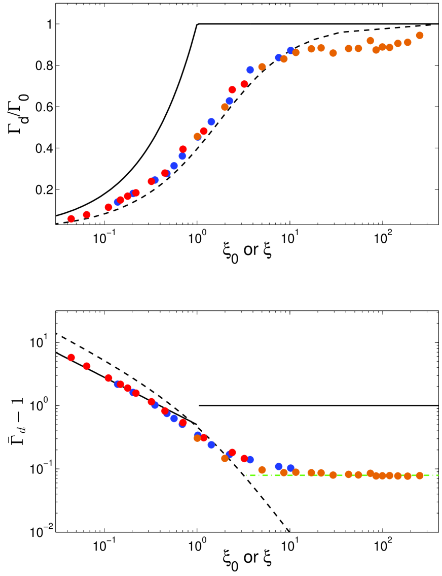
Figure 2: $\Gamma_{d}/\Gamma_{0}$ (Top panel) and $(\bar{\Gamma}_{d}-1)$ (Bottom panel) as functions of $\xi_{0}$ or $\xi$. The conventional estimates (black solid lines), the approximation (8) (black dashed lines), and the numerical results (orange dots: $r_{0}=10^{9}$cm, blue dots: $6\times 10^{11}$cm, and red dots: $6\times 10^{12}$cm). See the text concerning to the choice of $\xi_{0}$ or $\xi$.

where $\xi=(l/\Delta)^{1/2}\Gamma_{0}^{-4/3}$ and we have used $\bar{\Gamma}_{d}\sim(x+1/x)/2$. The corresponding results are shown in figure 2. For $\xi\ll 1$, we obtain $x\sim 0.47\xi^{3/4}$, while for $\xi\gg 1$, we obtain $x\sim 1$. In the rest of the paper, we call the estimates obtained in this section as the approximation (8) or the estimates based on Equation (8), while the estimates discussed in section 2 are called the conventional estimates. Since Equation (8) gives $x$ for a given $\xi$, to estimate $x$ at the deceleration radius $r_{d}$, we need to use the value of $\xi$ at $r_{d}$. In the thick shell regime $\xi_{0}<1$, $\xi$ is a constant during the deceleration process and we can use the initial value $\xi_{0}$. However, in the thin shell regime $\xi_{0}\gg 1$, due to the shell’s spreading $\Delta\sim\Delta_{0}+r_{d}/\Gamma_{0}^{2}\sim\Delta_{0}(1+\xi_{0}^{2})$, the value $\xi\sim\xi_{0}(1+\xi_{0}^{2})^{-1/2}$ is always about unity at $r_{d}$ (Sari & Piran 1995). Then, if we plot $x$ and the reverse shock temperature $(\bar{\Gamma}_{d}-1)$ as functions of the initial value $\xi_{0}$, they are expected to flatten in the intermediate regime. Since $\xi\sim\xi_{0}$ in the thick shell and intermediate regime, we can directly compare the two approximations, and we find that the conventional approximation overestimates $x$ and $(\bar{\Gamma}_{d}-1)$ in the intermediate regime. The conventional estimates are $x=\xi_{0}^{3/4}$ and $(\bar{\Gamma}_{d}-1)=\xi_{0}^{-3/4}/2$ for $\xi_{0}<1$ and $x\sim 1$ and $(\bar{\Gamma}_{d}-1)\sim 1$ for $\xi_{0}>1$.

Using the deceleration radius $r_{d}$ and the Lorentz factor $\Gamma_{d}$, the deceleration time is $t_{d}\sim r_{d}/(2c\Gamma_{d}^{2})=l/(2^{4/3}c\Gamma_{d}^{8/3})$. For the solution of Equation (8), we have an estimate of the correction factor $C_{t}=2^{-4/3}x^{-8/3}$. Assuming no gradients in the distribution functions of the pressure and velocity in the shock regions, we obtain $\nu_{m,r}/\nu_{m,f}\sim(\bar{\Gamma}_{d}-1)^{2}/\Gamma_{d}^{2}$ and $F_{\nu,max,r}/F_{\nu,max,f}\sim\Gamma_{d}^{2}/\Gamma_{0}$ where we have assumed $R_{B}=\epsilon_{B,r}/\epsilon_{B,f}=1$. Then, we get the correction factors $C_{m}\sim(1-x)^{4}/(4x^{4})$ and $C_{F}\sim x^{2}$.

5 Numerical Simulation

The two analytic estimates which we have discussed include approximations (e.g. a simplified shock approximation and no gradients in the distribution functions of hydrodynamics quantities in the shock regions). Furthermore, the estimate (8) gives the Lorentz factor $\Gamma_{d}$ for a given $\xi$ at the deceleration radius $r_{d}$, instead of the initial value $\xi_{0}$. Since the typical frequency of the reverse shock emission is sensitive to the temperature $(\bar{\Gamma}_{d}-1)$, it is important to investigate how $\xi$ at $r_{d}$ depends on $\xi_{0}$ (or where $\xi$ becomes a constant) and what asymptotic value the reverse shock temperature takes in the thin shell regime. To examine the accuracy of the approximations and evaluate the shock Lorentz factors and the corrections factors $C_{t}$, $C_{m}$ and $C_{F}$, we employ a spherical Lagrangian code based on the Godunov method with an exact Riemann solver (Kobayashi et al. 1999; Kobayashi & Sari 2000; Kobayashi & Zhang 2007). No MHD effects are included in our purely hydrodynamic calculations. However, if the magnetization of a fireball is not too large (i.e. the ratio of magnetic to kinetic energy flux $\sigma\lower 2.15277pt\hbox{$\;\buildrel<\over{\sim}\;$}0.1$; Giannios et al. 2008; Mimica et al. 2009), the dynamics of shocks is not affected by magnetic fields, and our numerical results can be used to model the synchrotron emission from forward and reverse shocks. We will evaluate the correction factors for $R_{B}=\epsilon_{B,r}/\epsilon_{B,f}=1$.

The initial configuration for our simulations is a static uniform fireball surrounded by a uniform cold ISM. The hydrodynamic evolution is evaluated through the stages of initial acceleration, coasting, energy transfer to the ISM and deceleration. The evolution of a fireball is fully discussed in Kobayashi et al. (1999). We assume explosion energy $E_{0}=10^{52}$ ergs and ambient density $n_{1}=1~{}\mbox{proton~{}cm}^{-3}$ for all the simulations, while we vary the dimensionless entropy ($40~{}<~{}\Gamma_{0}~{}<~{}10^{3}$) and the initial fireball size ($r_{0}~{}=~{}10^{9}$cm, $6\times 10^{11}$cm, or $6\times 10^{12}$cm) to cover a wide rage of $\xi_{0}$.

5.1 Spectra and Light Curves

We evaluate shock emission as a sum of photons from Lagrangian cells (fluid cells) in numerical calculations. First consider a single fluid cell with Lorentz factor $\Gamma$, internal energy density $e$, particle density $n$ and mass $m$ in a shocked region (forward or reverse shock). Electrons are assumed to be accelerated in the shock to a power-law distribution with index $p=2.5$ above a minimum Lorentz factor $\gamma_{m}$. We assume that constant fractions $\epsilon_{e}=6\times 10^{-2}$ and $\epsilon_{B}=6\times 10^{-3}$ of the shock energy are given to electrons and magnetic fields, respectively. Our results are insensitive to the exact values of the microphysical parameters as long as $R_{B}=1$, but they are included here for completeness. The typical random Lorentz factor and the energy of magnetic fields evolve as $\gamma_{m}\propto e/n$ and $B^{2}\propto e$. The typical synchrotron frequency in the observer frame is $\nu_{m}\propto\Gamma\gamma_{m}^{2}B$, and the peak spectral power is $F_{\nu,max}\propto N_{e}\Gamma B$ for a total number $N_{e}\sim m/m_{p}$ of electrons in the cell. As we use a Lagrangian code, $N_{e}$ remains constant throughout the numerical evolution. The flux at a given frequency above $\nu_{m}$ is $F_{\nu}=F_{\nu,max}(\nu/\nu_{m})^{-(p-1)/2}\propto m\Gamma^{(p+1)/2}e^{(5p-3)/4}n^{1-p}$ , while below $\nu_{m}$ we have a synchrotron low-energy tail as $F_{\nu}=F_{\nu,max}(\nu/\nu_{m})^{1/3}\propto m\Gamma^{2/3}e^{-1/3}n^{2/3}$. Then, the emission from a cell can be estimated by using hydrodynamic quantities.

We treat a fluid cell as a particle that continually emits photons. However, we only have the locations of the cell $\{r_{j}\}$ and flux estimates $\{F_{\nu,j}\}$ at discrete timesteps $\{t_{lab,j}\}$ where the subscript $j$ indicates quantities at lab timestep $j$ and $r_{j}$ indicates the inner boundary of the cell. We assume all the photons are emitted from the inner boundary (i.e. we neglect the radial width of the cell). Prior to the light curve construction we generate a series of (logarithmic) bins with boundaries $\{t_{k}\}$ in the observer time domain, and we assume bin $k$ is bounded by $t_{k}$ and $t_{k+1}$. We now consider the emission from a single fluid cell between two consecutive lab timesteps: $j$ and $j+1$. Since a photon emitted at timestep $j$ arrives at the observer at $t_{j}\equiv t_{lab,j}-r_{j}/c$, photons spread over observer time bins between $t_{j}$ and $t_{j+1}$. Note that the observational time $t_{j}$ monotonically increases with $j$. Assuming that the observed flux $F_{\nu}$ evolves linearly between $t_{j}$ and $t_{j+1}$, and that the observer detects photons between $\nu_{R}$ and $\nu_{R}+d\nu$, we can estimate the amount of energy deposited to each time bin.

By monitoring the entropy evolution of a fluid cell, we can determine when the cell is heated by a forward or reverse shock. Then, we take into account all the timesteps after the shock heating for the construction of the light curve of the single fluid cell. We can apply this technique to all the cells inside (or outside) the contact discontinuity, and the total energy from all the cells in each time bin is divided by the bin size to get the reverse (or forward) shock light curve. It is then the simple matter of finding the maximum flux to obtain the peak time $t_{p}$ of the reverse shock emission.

To numerically define a property $f$ of the fireball shell at the peak time, we consider an average value

$$\left\langle f\right\rangle=\frac{\sum f_{i}\delta E_{i}}{\sum\delta E_{i}}.$$ (9)

where the summation is taken over all the fluid cells $\{i\}$ which are inside the contact discontinuity (i.e. in the reverse shock region) and which have contributed to the peak flux and $\delta E_{i}$ is the contribution from fluid cell $i$ to the peak time bin.

At the peak time, we construct the spectrum. For this purpose, we set up a series of bins $\{\nu_{q}\}$ in the frequency domain. For the peak time bin (i.e. the time bin which gives the peak flux), we know which fluid cells have contributed, and at which lab timestep it has happened. Let us assume that a fluid cell deposits energy between lab timestep $j$ and $j+1$. Assuming a linear evolution of the luminosity $\int_{\nu_{q}}^{\nu_{q+1}}F_{\nu}d\nu$ between the timesteps, we can estimate how much energy is deposited in each frequency bin at the peak time (the peak time bin). After summing up all the energy deposited by the relevant fluid cells in each frequency bin, we divide the energy by the frequency bin size to get the spectrum at the peak time.

5.2 Comparison of the Estimates and the Correction Factors

Figure 2 shows the Lorentz factor $\Gamma_{d}$ and the reverse shock temperature $(\bar{\Gamma}_{d}-1)$ at the peak time $t_{p}$. For the numerical results (the dots), we have used Equation (9) with $(\bar{\Gamma}_{d}-1)=e/nm_{p}c^{2}$ to obtain the average values, and we have assumed $\Delta_{0}=r_{0}$ to estimate $\xi_{0}$. The numerical results and the conventional approximation are plotted against $\xi_{0}$, while the approximation (8) is plotted against $\xi$. As we have discussed in Section 4, when the initial value is high $\xi_{0}\gg 1$, the $\xi$ parameter is expected to decrease to order-of-unity during the evolution. One finds that such flattening in the numerical results occurs at a rather high value $\xi_{0}\sim$ several. The approximation (8), especially $(\bar{\Gamma}_{d}-1)$ in the intermediate regime and $\Gamma_{d}$ in almost the whole range, is in better agreement with the numerical results, compared to the conventional estimates. The green dashed-dotted line in the bottom panel indicates the numerical asymptotic value: $\left\langle\bar{\Gamma}_{d}-1\right\rangle\sim 8\times 10^{-2}$.

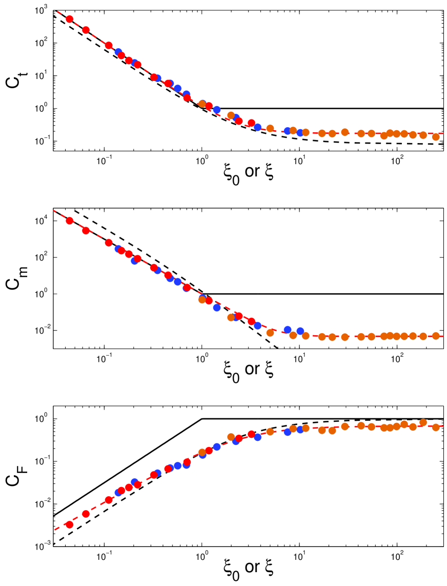
Figure 3: The correction factors as a function of $\xi_{0}$ or $\xi$. Top panel: The normalized peak time $C_{t}$, Middle panel: The normalized typical frequency ratio $C_{m}$, and Bottom panel: The normalized peak flux ratio $C_{F}$. The conventional estimates (black solid lines), the estimate based on the approximation (8) (black dashed lines), the numerical results (blue, red and orange dots are the same as in Figure 2), and numerical fitting formulae (red dashed lines).

Using a numerical peak time $t_{p}$, we estimate the correction factor $C_{t}=ct_{p}\Gamma_{0}^{8/3}/l$ as a function of $\xi_{0}$. The results are shown in the top panel of Figure 3. The conventional approximation well explains the numerical results in the thick shell regime $\xi_{0}<1$ but it breaks down in the thin shell regime $\xi_{0}>1$. In the thin shell regime, the numerical $C_{t}$ is lower by a factor of $\sim 5$ than the conventional estimate which is equivalent to the numerical peak time being earlier than expected. Since for simplicity we have neglected a factor of 2 in the conventional estimate as $t_{d}=l/c\Gamma_{0}^{8/3}$ instead of $l/2c\Gamma_{0}^{8/3}$, $C_{t}=0.5$ would be more appropriate for the conventional estimate in the thin shell regime. However, the numerical results are still smaller. This is in part due to the gradients in the distribution functions of hydrodynamics quantities in the reverse shock region. The numerical distributions have a higher value at the contact discontinuity, and they decrease toward the tail (see Figure 3 in Kobayashi & Zhang 2007). It makes the contribution of photons from the inner parts of the fireball shell less significant, reducing the effective width of the emission region in the shell, and the shock emission peaks earlier than in the homogeneous shell case. Since as we will see later, the magnetization estimate is rather insensitive to $C_{t}$ (and the peak time), we discuss only the line-of-sight emission in this paper. However, it is possible to include the high latitude emission at expense of computational time, and we have obtained very similar results for several selected cases. With the addition of the high latitude emission the overall light curve appears smoother with slightly shallower decay features. The position of the peak time increases by $\sim 50\%$.

Using the numerical values of the typical frequency ratio at the peak time, we estimate the correction factor $C_{m}=\Gamma_{0}^{2}\left[\nu_{m,r}(t_{p})/\nu_{m,f}(t_{p})\right]$ as a function of $\xi_{0}$. The results are shown in the middle panel of Figure 3. The conventional estimate is in good agreement with the numerical results in the thick shell regime, but as we expect from $C_{m}\varpropto(\bar{\Gamma}_{d}-1)^{2}$, it overestimates $C_{m}$ by a factor of $\sim 10^{2}$ in the thin shell regime. Finally the bottom panel of Figure 3 shows the results for $C_{F}=\Gamma_{0}^{-1}\left[F_{\nu,max,r}(t_{p})/F_{\nu,max,f}(t_{p})\right]$. The conventional approximation overestimates the amount of flux emitted by the reverse shock especially in the intermediate regime as Nakar & Piran (2004) have pointed out. The estimates based on Equation (8) provide a better approximation for all three correction factors in the intermediate regime. The red dashed lines in the three panels indicate the numerical fitting formulae $C_{t}=N_{t}+\xi_{0}^{-2}$ with $N_{t}\sim 0.2$, $C_{m}=N_{m}+\xi_{0}^{-3}$ with $N_{m}\sim 5\times 10^{-3}$ and $C_{F}^{-1}=N_{F}+M_{F}\xi_{0}^{-P_{F}}$ with $N_{F}\sim 1.5$, $M_{F}\sim 5$ and $P_{F}\sim 1.3$.

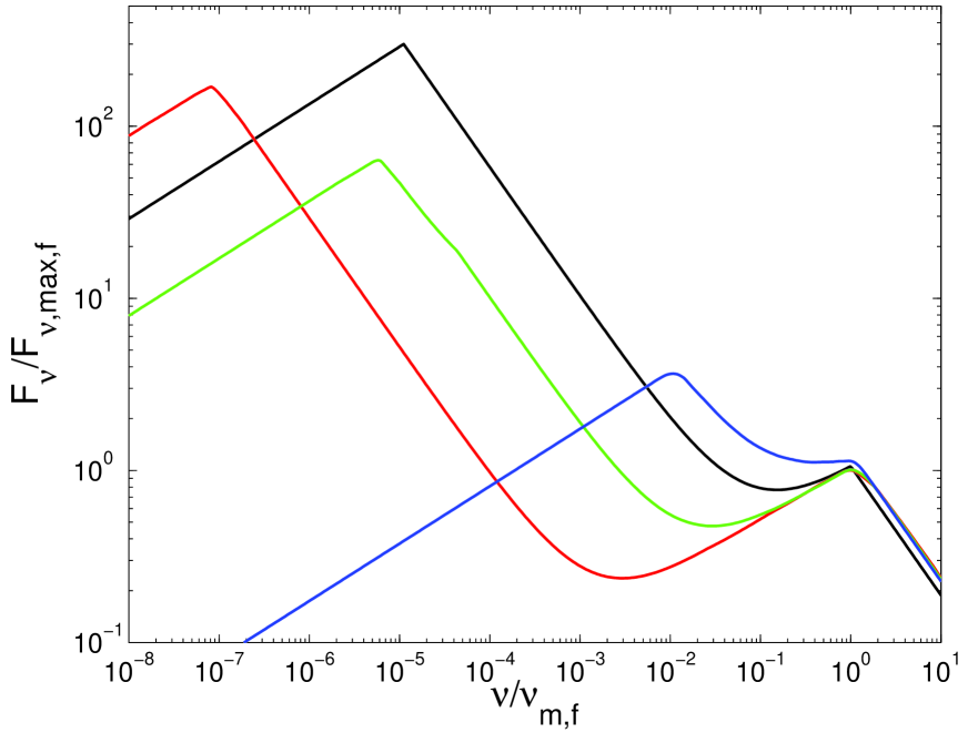
Figure 4: Numerical wide band spectra at the peak time: $\xi_{0}=0.1$ (blue line), 1 (green line) and 10 (red line). The black line shows the conventional estimate (thin shell case). The frequency and flux are normalized by the typical frequency and peak flux of the forward shock emission, respectively. $\Gamma_{0}=300$ and $\Delta_{0}\sim 3\times 10^{9}$cm (red line), $\sim 3\times 10^{11}$cm (green line), or $\sim 3\times 10^{13}$cm (blue line) are assumed.

Figure 4 illustrates wide band spectra at the peak time. We here consider three numerical cases with $\xi_{0}=0.1,1$ or 10. The black line indicates the conventional estimate in which the typical frequency $\nu_{m,r}$ of the reverse shock emission is lower by a factor of $\Gamma_{0}^{2}$ than that of the forward shock emission, and the peak flux $F_{\nu,max,r}$ of the reverse shock emission is higher by a factor of $\Gamma_{0}$. However, our numerical results show that in the thin shell regime $\nu_{m,r}$ is lower by a further factor of $\sim 10^{2}$ than the conventional estimate (the red line) , and that in the intermediate regime the peak flux $F_{\nu,max,r}$ would be lower by a factor of several (the green line). These indicate that the reverse shock emission would be elusive if the typical frequency of the forward shock is around the optical band and if the forward and reverse shock have the same microscopic parameters (Nakar & Piran 2004; Mimica et al. 2010; Melandri et al. 2010). In the thick shell regime, the peak frequency of the reverse shock emission is closer to that of the forward shock emission $\nu_{m,r}/\nu_{m,f}\sim\xi_{0}^{-3}\Gamma_{0}^{-2}$ (the blue line). We might have a better chance to detect the reverse shock component in early afterglow, although the light curve peaks earlier than in the thin shell regime.

5.3 Initial Lorentz Factor and Magnetization Parameter

The initial Lorentz factor can be evaluated by using the peak time $t_{p}\sim t_{d}$,

$$\Gamma_{0}=\left(\frac{C_{t}l}{ct_{p}}\right)^{3/8}$$ (10)

where $l$ is basically a known quantity from the prompt gamma-ray and late-time afterglow observations, and the estimate depends very weakly on more fundamental parameters $\Gamma_{0}\propto l^{3/8}\propto(E/n_{1})^{1/8}$, and we had obtained numerical result $C_{t}\sim 0.2+\xi_{0}^{-2}$. In principle, we can estimate $\xi_{0}$ from observable quantities. Since the duration $T$ of the prompt gamma-rays gives a rough estimate of the width $\Delta_{0}\sim cT$ (Kobayashi et al. 1997), using Equation (10) and the numerical $C_{t}(\xi_{0})$, we obtain $\xi_{0}\sim 5^{1/2}\sqrt{(t_{p}/T)-1}$ and $C_{t}\sim 0.2(1-T/t_{p})^{-1}$. In the thin shell regime, an early afterglow peaks well after the prompt gamma-ray emission (Sari 1997), and we have $C_{t}\sim 0.2$. However, in the thick shell regime, the peak time is almost equal to the width $\Delta_{0}/c$. The approximation $\Delta_{0}=cT$ might not be accurate enough to discuss the exact value of $\xi_{0}$. Since the flux before the optical peak $t_{p}$ is sensitive to the initial profile of the shell and in particular to $\xi_{0}$, the rising index of the light curve might be used to break the degeneracy of the $\xi_{0}$ estimate in the thick shell regime. Nakar & Piran (2004) have numerically estimated the rising index for a homogeneous shell in a range of $0.05<\xi_{0}<5$ as $\alpha_{rise}\sim 0.6\left[1+p(\xi_{0}-0.07\xi_{0}^{2})\right]$. A slow (rapid) rise is a signature of the thick (thin) shell regime (Kobayashi 2000).

The magnetization parameter $R_{B}$ can be estimated by using $\Gamma_{0}$ $R_{t}$, and $R_{F}$. For the typical decay index of the reverse shock emission $\alpha=2$, the conventional estimate is $R_{B,con}=(R_{F}^{3}\Gamma_{0}/R_{t}^{3})^{2/5}$ in the thin shell regime where $\Gamma_{0}=(l/ct_{p})^{3/8}$. Then, we obtain a correction factor for the magnetization parameter as

$$\frac{R_{B}}{R_{B,con}}=\frac{C_{t}^{3/20}}{C_{F}^{6/5}C_{m}^{4/5}}.$$ (11)

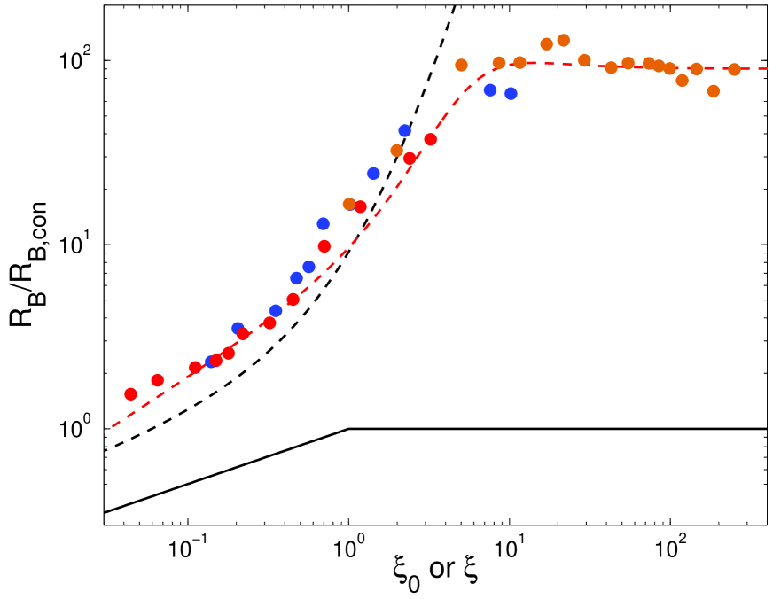
Figure 5: The correction factor for the magnetization parameter $R_{B}/R_{B,con}$ as a function of $\xi_{0}$ or $\xi$. The legend is the same as figure 3 with the best fit equation (red dashed line) obtained by the combination of the best fits to $C_{t},C_{m}$ and $C_{F}$. $\alpha=2$ is assumed.

One finds that the estimate is rather insensitive to $C_{t}$. In Figure 5, the numerical results are plotted with the approximations. For a typical GRB ($\xi_{0}\sim 1$), the conventional approximation (black solid line) underestimates the magnetization parameter by a factor of $\sim 10$. A more extreme discrepancy occurs in the thin shell regime, and the magnetization parameter is underestimated by a factor of $\sim 10^{2}$. The estimate based on Equation (8) (black dashed line) describes the numerical results reasonably well in the intermediate and thick shell regime.

6 Case Studies

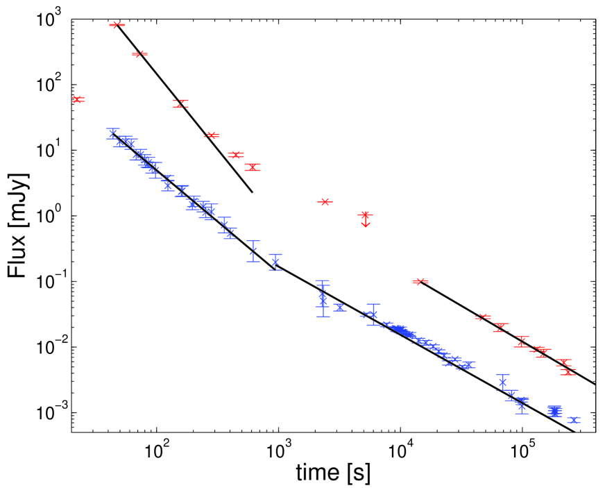
Figure 6: Light curves of early optical afterglows: GRB 990123 (red points) and GRB 090102 (blue points). The solid lines depict power-law fitting to the forward shock and reverse shock emission components. Data are from Kulkarni et al. 1999; Kobayashi & Sari 2000; Gendre et al. 2010 and references therein.

Swift revealed that the behavior of early afterglows are complicated than expected and there are indications of long-lasting central engine activity (e.g. flares and late-time energy injection; Zhang et al. 2006; Nousek et al. 2006; O’Brien et al. 2006). Although the nature of the central engine activity and additional components in early afterglows are interesting research subjects, in order to demonstrate our scheme which is based on an impulsive explosion model, we discuss early optical afterglows associated with GRB 990123 and GRB 090102. These light curves are described by a broken power-law with no flares (see Figure 6)

GRB 990123: This burst is one of the brightest GRBs observed so far. The basic parameters include $z=1.6$, $E\sim 1.4\times 10^{54}$ergs, and $T\sim 60$s (e.g. Kobayashi & Sari 2000 and references therein). The gamma-ray profile is dominated by two pulses, each lasting $\sim 8$s, separated by 12s. A bright optical flash is detected during the prompt emission (Akerlof et al. 1999), the optical emission peaks at $t_{p}\sim 50$s at 9 mag, and initially rapidly decays and it becomes shallower at a late time $t_{p,f}<0.1$ days. Using the bootstrap method for the light curve fitting, we find that $\alpha=2.31\pm 0.38$ and $\alpha_{f}=1.09\pm 0.07$ where the errors quoted are values to within 3 $\sigma$ of the best fits. We have only one optical data point before the peak, and it provides a lower limit of the rising index $\alpha_{rise}>2$ and the peak flux. We conservatively assume that the peak flux is 9 mag. Since the optical peak is comparable to the GRB duration (especially to the duration of the main two pulses) and the rising is rapid, this is an intermediate case $\xi_{0}\sim 1$, with the correction factors $C_{t}\sim 1.2$, $C_{m}\sim 1$ and $C_{F}\sim 0.16$. Using Equation (10) with a time-dilation correction, we obtain the initial Lorentz factor is about $\Gamma_{0}\sim 460n_{1}^{-1/8}$. Assuming $t_{p,f}=0.1$days, one has $R_{t}\sim 170$ and $R_{F}\sim 5000$, Equation (5) gives the magnetization parameter $R_{B}\sim 6300^{6600}_{6000}$ where the subscript and superscript indicate the range of the value when the error in $\alpha$ is taken into account. Since the forward shock peak is masked by the reverse shock emission, the peak time $t_{p,f}$ is rather uncertain. As we have discussed in Section 3, the magnetization estimate depends on $t_{p,f}$ as $R_{B}\propto t_{p,f}^{6(1+\alpha_{f}-\alpha)/(1+2\alpha)}\sim t_{p,f}^{-0.23}$. If the forward shock emission also peaks at $t_{p,f}\sim 50$s, the magnetization parameter $R_{B}$ is larger by a factor of $\sim 3$. Since Zhang et al. (2003) found a magnetization parameter of $R_{B}\sim 15^{2}=225$ based on the conventional approximation with $\xi_{0}\sim 1$, our magnetization estimate is larger by more than an order of magnitude.

GRB 090102: This burst shows a significant polarization at the $10\%$ level in the early optical afterglow and it suggests a magnetized fireball (Steele et al. 2009). The basic parameters include $z=1.5$, and $E\sim 5.8\times 10^{53}$ergs (e.g. Gendre et al. 2010 and references therein). The prompt gamma-ray emission lasts for $27$s and comprises four overlapping peaks starting 14s before the GRB trigger. The optical light curve, beginning at 13 mag, 40s after the GRB trigger, can be fitted by a broken power-law whose flux decays as a function of time ($F\propto t^{-\alpha}$) with a gradient $\alpha=1.56\pm 0.06$ that then flattens to $\alpha_{f}=1.04\pm 0.09$ (the solid lines; a break time is assumed to be $10^{3}$s). If we assume that the optical emission peaks at the first data point (the mid time is $t_{p}\sim 60$s after the beginning of the GRB) and $t_{p,f}=10^{3}$s, we obtain $\xi_{0}\sim 2.4$ and the correction factors: $C_{t}\sim 0.3,C_{m}\sim 8\times 10^{-2}$, and $C_{F}\sim 0.3$. Using $R_{t}\sim 17,R_{F}\sim 91$ and $\Gamma_{0}\sim 230n_{1}^{-1/8}$, we obtain $R_{B}\sim 220^{310}_{150}$. Since the optical emission has already decayed at the beginning of the observations, the actual peak time $t_{p}$ might be earlier. If we assume that it peaks at the end of the prompt gamma-ray emission $t_{p}\sim 30$s, it would be in the intermediate regime $\xi_{0}\sim 1$ and $\Gamma_{0}\sim 290n_{1}^{-1/8}$. Assuming $t_{p,f}=10^{3}$s, we obtain $R_{B}\sim 140^{180}_{110}$. The magnetization estimates depend on $t_{p,f}$ as $R_{B}\propto t_{p,f}^{0.7}$. If $t_{p,f}=10^{2}$s, $R_{B}$ is smaller by a factor of $\sim 5$.

The $\sigma$ parameter: The broadband afterglow emission of GRB 990123 is modeled to find $\epsilon_{B,f}\sim 10^{-6}$ (Panaitescu & Kumar 2004). Although there are no estimates available for GRB 090102, the broadband modeling generally shows that it is in a range of $\epsilon_{B,f}=10^{-5}-10^{-1}$ (Panaitescu & Kumar 2002). Using the estimated value of the magnetization parameter $R_{B}$, the ratio of magnetic to kinetic energy flux is $\sigma\sim 10^{-3}(g/0.25)(R_{B}/6300)(\epsilon_{B,f}/10^{-6})$ for GRB 990123 where $g\equiv(\bar{\Gamma}_{d}-1)/\bar{\Gamma}_{d}\sim 0.25$ for $\xi_{0}\sim 1$. For GRB 090102, assuming $g\sim 0.15~{}(\xi_{0}\sim 2.4)$ and $R_{B}\sim 220$, it is in a range of $\sigma\sim 3\times 10^{-4}-3$. Although magnetic pressure would suppress the formation of a reverse shock if $\sigma\mbox{\raisebox{-4.30554pt}{$\stackrel{{\scriptstyle>}}{{\sim}}$}}0.1$ (Giannios et al. 2008; Mimica et al. 2009), the low values are consistent (or the result includes the parameter region consistent) with the basic assumption in our analysis (i.e. magnetic fields do not affect the reverse shock dynamics). If a future event indicates a high value $\sigma\mbox{\raisebox{-4.30554pt}{$\stackrel{{\scriptstyle>}}{{\sim}}$}}0.1$, an interesting possibility to reconcile the problem is that the prompt optical emission (and prompt gamma-rays) would be produced through a dissipative MHD processes rather than shocks (Giannios & Spruit 2006; Lyutikov 2006; Giannios 2008; Zhang & Yan 2011).

Our magnetization estimates are slightly lowered if the blast wave radiates away a significant fraction of the energy in the early afterglow $E\propto t^{-17\epsilon_{e}/16}$ (Sari 1997). For $\epsilon_{e}=0.1$, the blast wave energy becomes smaller by a factor of $1.7$ between $t=50$s and $0.1$days, by a factor of $1.3$ between $t=60$s and $10^{3}$s, then the estimates of $R_{B}$ and $\sigma$ are reduced by a factor of $1.5-2$.

7 Conclusions

We have discussed a revised method to estimate the magnetization degree of a GRB fireball. We use the ratios of observed properties of early afterglow so the poorly known parameters for the shock microphysics (e.g. $\epsilon_{e}$ and $p$) would cancel out. Since the estimate depends only weakly on the explosion energy and the fireball deceleration time, the estimate does not require the exact distance (redshift) to the source as an input parameter. Since most observed events fall in the intermediate regime between the thin and thick shell extremes, we have provided a new approximation for the spectral properties of the forward shock and reverse shock emission, which well describes the numerical results in the intermediate regime. The previous standard approach underestimates the degree of fireball magnetization $R_{B}$ by a factor of $10\sim 100$. We have estimated $\sigma\sim 10^{-3}$ for GRB 990123. For GRB 090102, it is not well constrained due to the uncertainty in $\epsilon_{B,f}$, and it is in a range of $\sigma\sim 3\times 10^{-4}-3$.

In the GRB phenomena, extreme relativistic motion with $\Gamma_{0}>100$ is necessary to avoid the attenuation of hard gamma-rays. The acceleration process is likely to induce a small velocity dispersion inside the outflow $\Delta\Gamma\sim\Gamma$ (e.g. thermal acceleration). If internal shocks are responsible for the production of the prompt gamma-rays, the dispersion should be even larger (Beloborodov 2000; Kobayashi & Sari 2001). The velocity dispersion leads to the spreading of the shell structure in the coasting phase and the $\xi$ parameter decreases as $\xi\propto\Delta^{-1/2}$. As an order-of-magnitude estimate, when the initial value $\xi_{0}>1$, the reverse shock always becomes mildly relativistic $(\xi\sim 1)$ at the deceleration radius and the reverse shock temperature $(\bar{\Gamma}_{d}-1)$ is expected to be insensitive to the initial value $\xi_{0}$. However, it is difficult to analytically quantify the asymptotic reverse shock temperature. We have numerically shown that the spreading effect becomes significant at rather high values $\xi_{0}\lower 2.15277pt\hbox{$\;\buildrel>\over{\sim}\;$}$ several, and that the asymptotic value is $(\bar{\Gamma}_{d}-1)\sim 8\times 10^{-2}$.

We have confirmed that, especially in the intermediate regime $\xi_{0}\sim 1$, the reverse shock emission is much weaker than the standard estimates as Nakar & Piran (2004) had pointed out, and that in the thin shell regime the typical frequency of the reverse shock emission is much lower than the standard estimates. If the fireball is not magnetized $R_{B}=\epsilon_{B,r}/\epsilon_{B,f}=1$, the reverse shock emission more easily falls below the forward shock emission. The lack of optical flashes from most GRBs might be partially explained in a revised non-magnetized model. If the fireball shell does not spread even in the thin shell regime (i.e. the velocity distribution is completely uniform), only a small fraction of the kinetic energy of the shell is converted to thermal energy in the reverse shock, and the reverse shock emission is practically suppressed in the thin shell regime $\xi_{0}\gg 1$.

We thank Ehud Nakar and Elena M. Rossi for useful discussion. This research was supported by STFC fellowship and grant.

References

- Akerlof et al. (1999) Akerlof, C., Balsano, R., Barthelmy, S., et al. 1999, Nature, 398, 400
- Beloborodov (2000) Beloborodov,A.M. 2000, ApJ, 539, L25
- Blandford & McKee (1976) Blandford, R. D., & McKee, C. F. 1976, Physics of Fluids, 19, 1130
- (4) Drenkhahn, G. & Spruit, H.C. 2002, A&A, 391, 1141
- Fan et al. (2002) Fan, Y.-Z., Dai, Z.-G., Huang, Y.-F., & Lu, T. 2002, Chinese J. Astron. Astrophys., 2, 449
- Fan et al. (2004) Fan, Y.-Z., Wei,D.M., & Wang, C.F. 2004, A&A, 424, 477
- Fan et al. (2005) Fan, Y.-Z., Zhang, B., & Wei, D.M. 2005, ApJ, 628, L25
- Fox et al. (2003) Fox, D. W., Price, P. A., Soderberg, A. M., et al. 2003, ApJ, 586, L5
- Gendre et al. (2010) Gendre, B., Klotz, A., Palazzi, E., et al. 2010, MNRAS, 405, 2372
- (10) Giannios, D. & Spruit,H.C. 2006, A&A, 450, 887
- Giannios (2008) Giannios, D. 2008, A&A, 480, 305
- Giannios et al. (2008) Giannios, D., Mimica, P., & Aloy, M. A. 2008, A&A, 478, 747
- Gomboc et al. (2008) Gomboc, A., Kobayashi, S., Guidorzi, C., et al. 2008, ApJ, 687, 443
- Götz et al. (2009) Götz, D., Laurent, P., Lebrun, F., Daigne, F., & Bošnjak, Ž. 2009, ApJ, 695, L208
- (15) Granot, J. 2012, MNRAS, 421, 2442
- Kalemci et al. (2007) Kalemci, E., Boggs, S. E., Kouveliotou, C., Finger, M., & Baring, M. G. 2007, ApJS, 169, 75
- Kobayashi (2000) Kobayashi, S. 2000, ApJ, 545, 807
- Kobayashi et al. (1997) Kobayashi, S., Piran, T., & Sari, R. 1997, ApJ, 490, 92
- Kobayashi et al. (1999) Kobayashi, S., Piran, T., & Sari, R. 1999, ApJ, 513, 669
- Kobayashi & Sari (2000) Kobayashi, S., & Sari, R. 2000, ApJ, 542, 819
- (21) Kobayashi, S., & Sari, R. 2001, ApJ, 551, 934
- Kobayashi & Zhang (2003) Kobayashi, S., & Zhang, B. 2003, ApJ, 597, 455
- Kobayashi & Zhang (2007) Kobayashi, S., & Zhang, B. 2007, ApJ, 655, 973
- Komissarov et al. (2009) Komissarov, S. S., Vlahakis, N., Königl, A., & Barkov, M. V. 2009, MNRAS, 394, 1182
- Kulkarni et al. (1999) Kulkarni, S. R., Djorgovski, S. G., Odewahn, S. C., et al. 1999, Nature, 398, 389
- Kumar & Panaitescu (2003) Kumar, P., & Panaitescu, A. 2003, MNRAS, 346, 905
- Kumar & Barniol Duran (2009) Kumar, P., & Barniol Duran, R. 2009, MNRAS, 400, L75
- Lazzati (2006) Lazzati, D. 2006, New J. Phys, 8, 131
- Li et al. (2003) Li, W., Filippenko, A. V., Chornock, R., & Jha, S. 2003, ApJL, 586, L9
- Lyutikov (2006) Lyutikov, M. 2006, New J. of Phys, 8, 119
- McGlynn et al. (2007) McGlynn, S., Clark, D. J., Dean, A. J., et al. 2007, A&A, 466, 895
- (32) McKinney, J.C., & Blandford, R.D. 2009, MNRAS, 394, L126
- Medvedev & Loeb (1999) Medvedev,M.V., & Loeb,A. 1999, ApJ, 526, 697
- Melandri et al. (2010) Melandri, A., Kobayashi, S., Mundell, C. G., et al. 2010, ApJ, 723, 1331
- Mészáros & Rees (1999) Mészáros, P., & Rees, M. J. 1999, MNRAS, 306, L39
- Mimica et al. (2009) Mimica, P., Giannios, D., & Aloy, M. A. 2009, A&A, 494, 879
- (37) Mimica, P., Giannios, D., & Aloy, M. A. 2010, MNRAS, 407, 2501
- Nakar & Piran (2004) Nakar, E., & Piran, T. 2004, MNRAS, 353, 647
- Nakar & Piran (2005) Nakar, E., & Piran, T. 2005, ApJ, 619, L147
- Narayan et al. (2011) Narayan, R., Kumar, P. & Tchekhovskoy, A. 2011, MNRAS, 416, 2193
- Nishikawa et al. (2005) Nishikawa, K.I. et al. 2005, ApJ, 622, 927
- Nousek et al. (2006) Nousek, J.A. et al. 2006, ApJ, 642, 389
- O’Brien et al. (2006) O’Brien, P.T. et al. 2006, ApJ, 647, 1213
- Panaitescu & Kumar (2002) Panaitescu, A., & Kumar, P. 2002, ApJ, 571, 779
- Panaitescu & Kumar (2004) Panaitescu, A., & Kumar, P. 2004, MNRAS, 353, 511
- Piran (2004) Piran, T. 2004, Reviews of Modern Physics, 76, 1143
- Sari (1997) Sari, R. 1997, ApJ, 489, L37
- Sari & Piran (1995) Sari, R., & Piran, T. 1995, ApJ, 455, L143
- Sari et al. (1998) Sari, R., Piran, T., & Narayan, R. 1998, ApJ, 497, L17
- Sari & Piran (1999) Sari, R., & Piran, T. 1999, ApJ, 520, 641
- Soderberg & Ramirez-Ruiz (2002) Soderberg, A. M., & Ramirez-Ruiz, E. 2002, MNRAS, 330, L24
- Spitkovsky (2008) Spitkovsky, A. 2008, ApJ, 682, L5
- Steele et al. (2009) Steele, I. A., Mundell, C. G., Smith, R. J., Kobayashi, S., & Guidorzi, C. 2009, Nature, 462, 767
- Tchekhovskoy et al. (2008) Tchekhovskoy, A., McKinney, J. C., & Narayan, R. 2008, MNRAS, 388, 551
- Toma et al. (2009) Toma, K. et al. 2009, ApJ, 698, 1042
- Yonetoku et al. (2011) Yonetoku, D., Murakami, T., Gunji, S., et al. 2011, ApJ, 743, L30
- (57) Zhang, B., Kobayashi, S., & Mészáros, P. 2003, ApJ, 595, 950
- Zhang et al. (2003) Zhang, B.,& Kobayashi, S. 2005, ApJ, 628, 315
- Zhang & Mészáros (2004) Zhang, B., & Mészáros, P. 2004, International Journal of Modern Physics A, 19, 2385
- Zhang et al. (2006) Zhang, B., et al. 2006, ApJ, 642, 354
- Zhang & Pe’er (2009) Zhang, B., & Pe’er, A. 2009, ApJ, 700, L65
- Zhang & Yan (2011) Zhang, B., & Yan, H. 2011, ApJ, 726, 90