Implications of Bilinear R-Parity Violation on Neutrinos and Lightest Neutralino Decay in Split Supersymmetry

Abstract

We discuss neutrino parameters in addition with the effects of a Higgs boson of mass $\sim$ 125 GeV in Split Supersymmetry with Bilinear R-Parity Violation. This model allows for the explanation of neutrino masses and mixing angles, and has the gravitino as Dark Matter candidate. We find constraints on the parameters in the neutrino sector of the model by performing a numerical study of the parameter space, and by fitting neutrino oscillation observables and the Higgs mass. In addition, we study in detail the decay of the lightest neutralino in this model and we realize the importance of the exact neutralino/chargino spectrum in the computation of its branching ratios.

1 Introduction

It is an indisputable fact that the ATLAS and CMS Collaborations of the Large Hadron Collider (LHC) have discovered a new particle [1, 2, 3, 4], with mass near 125 GeV and consistent with the Higgs boson [5, 6, 7, 8, 9, 10] of the Standard Model [11, 12, 13, 14]. Its measured value has considerable impact on supersymmetric models, such as the Minimal Supersymmetric Standard Model (MSSM). In addition, current LHC searches pushes supertparner masses above 1 TeV [15, 16, 17, 18, 19, 20, 21, 22]. This fact leaves the naturalness of the minimal theory in tension and points to an empirically favored supersymmetric scenario called Split Supersymmetry (SS) [23, 24], where all sfermions are very heavy, placed universally at a scale $\tilde{m}$, while charginos and neutralinos remain light. Although SS is unnatural by construction and hierarchy is not longer a guiding principle (so the Higgs mass has to be fined-tuned), this model retains unification of gauge couplings, naturally suppressed flavour mixing and a Dark Matter candidate. For completeness, we mention also the alternative scenarios Inverted Hierarchy [25, 26], High Scale Supersymmetry [27], and Intermediate Scale Supersymmetry [28].

A very striking effect of Split Supersymmetry is the long lifetime of the gluino [29]. Since all squarks are very heavy, with a mass of order of the split supersymmetric scale $\widetilde{m}$, the gluino will decay via off-shell squarks, and with an increasing lifetime as $\widetilde{m}$ increases. Searches have been made for long lived gluinos at the LHC with negative results. CMS rules out gluino R-hadrons with mass $m_{\tilde{g}}<1$ TeV if their lifetime satisfies $10^{-6}<\tau_{\tilde{g}}<10^{3}$ sec [30]. ATLAS rules out stable gluinos (gluinos that escape the detector before decaying) with mass $m_{\tilde{g}}\lesssim 1270$ GeV [31]. Searches with gluinos decaying fast have been made at ATLAS also with negative results [32, 16, 33]. Analogous searches by CMS give equally negative results, with gluino masses bounded from below by 1.26 TeV, unless the LSP has a large mass, in which case the bound decreases [34]. See also [35, 36, 37, 38, 39, 40, 41].

If one allows R-parity to be not conserved, neutrino masses can be generated [42, 43, 44, 45, 46]. This can be done without introducing problems with too fast proton decay [47]. This is so because neutrino masses need only Lepton number violation, while proton decay needs both Lepton and Baryon number violation. Another issue to be considered is that, if R-Parity is conserved, the lightest neutralino is a Dark Matter candidate [48, 49], but this is no longer the case if R-Parity is violated. Nevertheless, in models with R-Parity violation the gravitino can be a good dark matter candidate since it can live longer than the age of the universe [50, 51, 52]. If one ask the gravitino to be responsible for the positron excess seen by the AMS2 experiment [53], then BRpV would not be enough [54]. Nevertheless, it is not clear that the excess is due to Dark Matter [55], and gravitino as Dark Matter candidate works as long as its mass is not larger than ${\cal{O}}(10)$ GeV [50].

In this article we study the implications of a Higgs boson mass of $\sim$ 125 GeV on a Split Supersymmetric model, which includes R-Parity bilinearly violated terms (SS-BRpV). It has been shown possible to accommodate the observed Higgs mass in SS, which imposes constrains in the ($\tilde{m},\tan\beta$) plane [56, 57, 58]. We check that in this case the split supersymmetric scale $\widetilde{m}$ is rather low ($<10^{6}$ GeV). We also check that the case $\tan\beta=1$ is not ruled out, as it is in the MSSM, because of lack of cancellation between quark and squark loops. The price to pay may be the divergence of the top quark Yukawa coupling at scales larger than $\widetilde{m}$ but smaller than $M_{P}$. This does not excludes the scenario, but implies the appearance of new physics at that scale.

We also discuss neutrino masses and mixing angles in SS-BRpV. Neutrino masses arises in this model due to mixing in the neutralino/neutrino sector with the inclusion of a gravity induced term [59]. We discuss how the effect of introducing a constraint on the Higgs mass affects the model parameters, requiring that current experimental values from neutrino physics given in [60, 61] are reproduced with a 95% confidence level. In particular, we see the model forces a strong dependence on the atmospheric and solar neutrino mixing angles. In addition, we study in detail the two-body decays of the lightest neutralino. We conduct a general scan of our available parameter space and realize the importance in knowing the exact neutralino/chargino spectrum in the computation of the neutralino branching fractions.

2 Split Supersymmetry and the Higgs Mass

The split supersymmetric lagrangian below the $\widetilde{m}$ scale includes charginos, neutralinos, plus all the SM particles, including the SM-like Higgs boson $H$ [23, 24]. The lagrangian looks as follows,

$${\cal L}^{split}_{susy} = {\cal L}^{split}_{kinetic}\ +\ m^{2}H^{\dagger}H-\frac{\lambda}{2}(H^{\dagger}H)^{2}-\Big{[}Y_{u}\overline{q}_{L}u_{R}i\sigma_{2}H^{*}\ +\ Y_{d}\overline{q}_{L}d_{R}H\ +\ Y_{e}\overline{l}_{L}e_{R}H\ +\$$

$$+\frac{M_{3}}{2}\widetilde{G}\widetilde{G}\ +\ \frac{M_{2}}{2}\widetilde{W}\widetilde{W}\ +\ \frac{M_{1}}{2}\widetilde{B}\widetilde{B}\ +\ \mu\widetilde{H}_{u}^{T}i\sigma_{2}\widetilde{H}_{d}\ +\$$

$$+\textstyle{\frac{1}{\sqrt{2}}}H^{\dagger}(\tilde{g}_{u}\sigma\widetilde{W}\ +\ \tilde{g}^{\prime}_{u}\widetilde{B})\widetilde{H}_{u}\ +\ \textstyle{\frac{1}{\sqrt{2}}}H^{T}i\sigma_{2}(-\tilde{g}_{d}\sigma\widetilde{W}+\tilde{g}^{\prime}_{d}\widetilde{B})\widetilde{H}_{d}+\mathrm{h.c.}\Big{]},$$

In the gaugino sector we use as input the low energy values for the Bino and Wino masses $M_{1}$ and $M_{2}$, and the higgsino mass $\mu$. At a scale $M_{\chi}$ we decouple the gauginos and higgsinos, such that below that scale the SM is valid. To calculate the Higgs mass in this model we first need the RGE evolution of the quartic Higgs coupling, and second the quantum corrections, that we approximate at one loop following a prescription for the renormalization scale given in ref. [62].

In Split Supersymmetry a unification of gauge couplings is assumed [23]. We start at the electroweak scale $m_{Z}$ with SM-RGE, changing at the scale $M_{\chi}$ to SS-RGE, and changing again at the $\widetilde{m}$ scale to the MSSM-RGE [24]. The initial condition is given by the values of the gauge couplings $g_{1}$, $g_{2}$, and $g_{3}$, at the weak scale. We calculate the electroweak couplings with the help of $\alpha_{\text{fin}}^{-1}(m_{Z})=128.962\pm 0.014$ [63], and $\sin^{2}\theta_{w}(m_{Z})=0.23119\pm 0.00014$ [64], namely $g_{2}^{2}=4\pi\alpha_{fin}/s^{2}_{w}$ and $g_{1}^{2}=5g^{\prime 2}/3$, $g^{\prime 2}=4\pi\alpha_{fin}/c^{2}_{w}$. In turn, the strong coupling constant satisfy $g_{3}^{2}=4\pi\alpha_{s}$, with $\alpha_{s}(m_{Z})=0.1184\pm 0.0007$ [64]. The intersection of the three gauge coupling RGE curves defines the Grand Unification scale $M_{GUT}$. Since the unification is not perfect (within experimental errors), we define $M_{GUT}$ as the average of the three meeting points.

Matching conditions at the scale $\widetilde{m}$ between SS and the MSSM are,

$$\tilde{g}_{u}(\tilde{m})=g(\tilde{m})\ \sin\beta ,\qquad \tilde{g}_{d}(\tilde{m})=g(\tilde{m})\ \cos\beta$$

$$\tilde{g}^{\prime}_{u}(\tilde{m})=g^{\prime}(\tilde{m})\ \sin\beta ,\qquad \tilde{g}^{\prime}_{d}(\tilde{m})=g^{\prime}(\tilde{m})\ \cos\beta,$$ (2)

The large difference that may appear between up and down $\tilde{g}$ couplings at $\widetilde{m}$ is due to the value of $\tan\beta$.

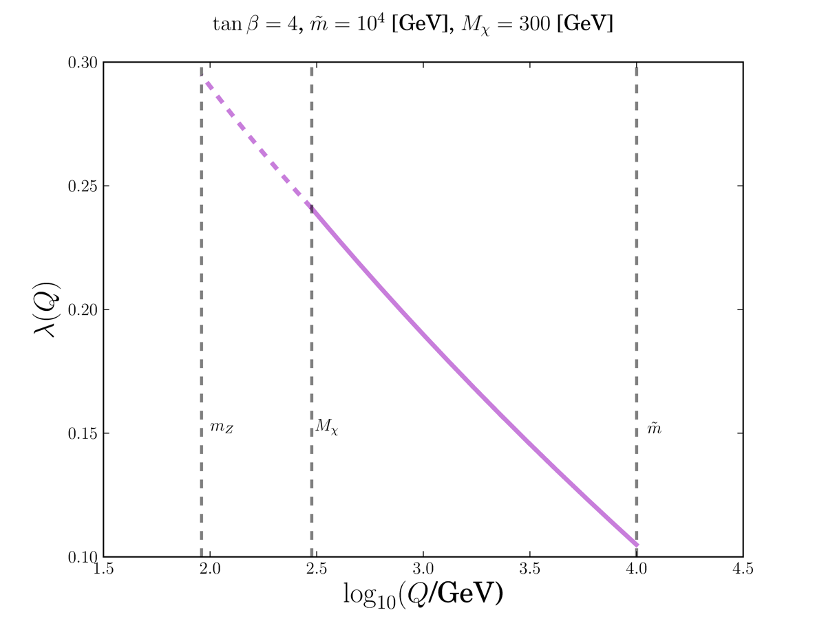
Figure 1: Running of the Higgs coupling $\lambda$, for $\tan\beta=4$, $\widetilde{m}=10^{4}$ GeV and $M_{\chi}=300$ GeV.

In fig. 1 we see the running of the Higgs quartic coupling $\lambda$ for the set of input parameters $\tan\beta=4$, $\widetilde{m}=10^{4}$ GeV, and $M_{\chi}=300$ GeV. The starting point is also at $\widetilde{m}$ with the matching condition,

$$\lambda(\widetilde{m})=\frac{1}{4}\left[g^{2}(\widetilde{m})+g^{\prime 2}(\widetilde{m})\right]\cos^{2}2\beta$$ (3)

As we can see, the threshold at $M_{\chi}$ has just a small effect. The renormalized Higgs mass includes the tree-level contribution proportional to the quartic coupling $\lambda$ evaluated at the chosen renormalization scale $Q=m_{t}$, following ref. [62]. The value of the Higgs coupling at the renormalization scale is $\lambda=0.264$, leading to a Higgs boson mass $m_{H}=125.3$ GeV, consistent with observations from the LHC.

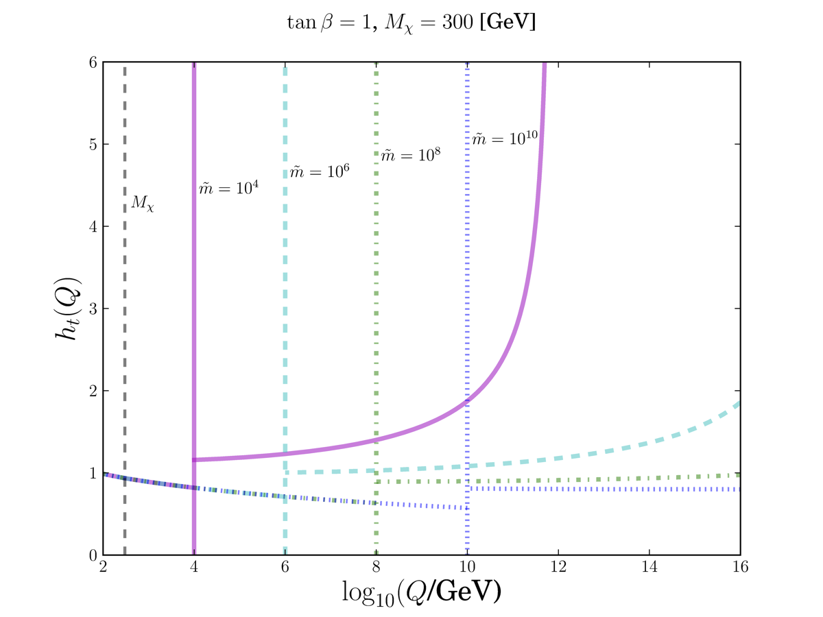
Figure 2: Running of the top quark Yukawa coupling $h_{t}$ for $\tan\beta=1$ and several values of the Split Supersymmetric scale $\widetilde{m}$.

For extreme values like $\tan\beta=1$, we can have a value for the Higgs mass consistent with the experimental evidence, nevertheless, unification of gauge couplings fails because the top quark Yukawa coupling becomes non-perturbatively large at a scale larger than $\widetilde{m}$. This fact can be seen in fig. 2 for different values of the SS scale. The fact that the top Yukawa coupling diverges is an indication of new physics appearing at that scale. The model ceases to be valid beyond that scale. In the figure we show also the threshold at $\widetilde{m}$. Below it, the SS-RGE controls the behavior of the top quark Yukawa $h_{t}$ and its evolution is the same for any of the chosen values for $\widetilde{m}$. After that threshold we switch to the MSSM-RGE for $h_{t}$ which hold the following boundary condition,

$$h_{t}^{SS}(\widetilde{m})=h_{t}^{MSSM}(\widetilde{m})\cos\beta$$ (4)

and this explains the discontinuity for $h_{t}$ at the threshold. We stress the fact that the divergence for $h_{t}$ at a scale larger than $\widetilde{m}$ does not invalidates the low scale SS model.

A Higgs mass compatible with experiments is obtained for a SS scale $10^{4}\lesssim\widetilde{m}\lesssim 10^{6}$ GeV, and any value of $\tan\beta$ is possible (a SS model with $\widetilde{m}$ smaller than $10^{4}$ is not much different to the MSSM). The fact that $\tan\beta=1$ with $\widetilde{m}\sim 10^{6}$ is consistent with the experimental measurements for the Higgs mass is an interesting fact, although already noticed in the literature [24]. The price we pay in this case is that the top quark Yukawa coupling becomes non-perturbative at scales larger than $\widetilde{m}$ and as a consequence the gauge coupling unification is lost.

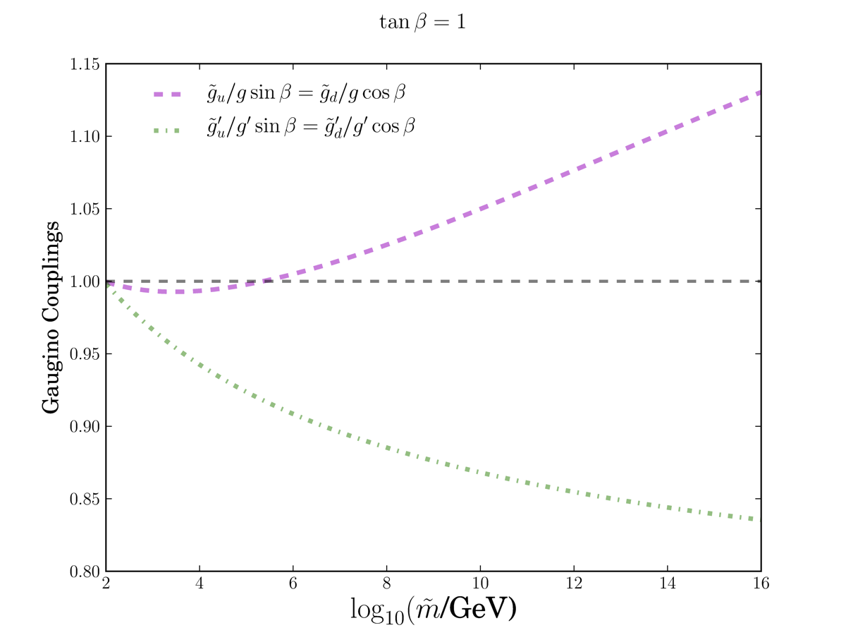
Figure 3: Ratio between the gaugino couplings and the gauge couplings, weighted by $\sin\beta$ or $\cos\beta$, as a function of the SS scale $\widetilde{m}$, calculated at the weak scale for $\tan\beta=1$.

In fig. 3 we have the Higgs-higgsino-gaugino couplings for the special case $\tan\beta=1$. From eq. (2) we see that in this case both couplings $\tilde{g}$ and both $\tilde{g}^{\prime}$ are equal to each other at $\widetilde{m}$, and since RGE are also the same, the couplings remain equal, as can be seen in the figure. From the values $\widetilde{m}\lesssim 10^{6}$ GeV we also expect in this case deviations of at most $10\%$.

3 Neutrino Masses in Bilinear R-Parity Violation

If R-Parity is bilinearly violated, very little of the above conclusions are changed, since the RGE are the same. In SS-BRpV, the decoupling of the sleptons induce BRpV couplings between gauginos, higgsinos and Higgs, which at lower scales look like [65],

$${\cal L}^{split}_{RpV}=\epsilon_{i}\widetilde{H}_{u}^{T}i\sigma_{2}L_{i}\ -\ \textstyle{\frac{1}{\sqrt{2}}}a_{i}H^{T}i\sigma_{2}(-\tilde{g}_{d}\sigma\widetilde{W}+\tilde{g}^{\prime}_{d}\widetilde{B})L_{i}\ +\ h.c.,$$ (5)

where $a_{i}$ are dimensionless parameters that characterize the decoupling of the sleptons. These terms induce a neutralino/neutrino mixing when the Higgs field acquire a vacuum expectation value,

$${\cal L}^{split}_{RpV}=-\left[\epsilon_{i}\widetilde{H}_{u}^{0}+\frac{1}{2}a_{i}v\left(\tilde{g}_{d}\widetilde{W}_{3}-\tilde{g}^{\prime}_{d}\widetilde{B}\right)\right]\nu_{i}\ +\ h.c.\ +\ \ldots$$ (6)

where $v$ is normalized such that the $W$ gauge boson has a mass $m_{W}=\frac{1}{2}gv$, thus $v\approx 246$ GeV. In this way, the neutralino/neutrino sector in the basis $\psi=(-i\lambda^{\prime},-i\lambda^{3},\widetilde{H}_{d}^{0},\widetilde{H}_{u}^{0},\nu_{e},\nu_{\mu},\nu_{\tau})$ develops a mass matrix that we write as follows,

$${\cal M}_{N}^{SS}=\left[\begin{array}[]{cc}{\mathrm{M}}_{\chi^{0}}^{SS}&(m^{SS})^{T}\\ m^{SS}&0\end{array}\right],$$ (7)

where ${\mathrm{M}}_{\chi^{0}}^{SS}$ is the neutralino mass sub-matrix,

$${\bf M}_{\chi^{0}}^{SS}=\left[\begin{array}[]{cccc}M_{1}&0&-\frac{1}{2}\tilde{g}^{\prime}_{d}v&\frac{1}{2}\tilde{g}^{\prime}_{u}v\\ 0&M_{2}&\frac{1}{2}\tilde{g}_{d}v&-\frac{1}{2}\tilde{g}_{u}v\\ -\frac{1}{2}\tilde{g}^{\prime}_{d}v&\frac{1}{2}\tilde{g}_{d}v&0&-\mu\\ \frac{1}{2}\tilde{g}^{\prime}_{u}v&-\frac{1}{2}\tilde{g}_{u}v&-\mu&0\end{array}\right],$$ (8)

and $m^{SS}$ includes the mixing between neutralinos and neutrinos,

$$m^{SS}=\left[\begin{array}[]{cccc}-\frac{1}{2}\tilde{g}^{\prime}_{d}a_{1}v&\frac{1}{2}\tilde{g}_{d}a_{1}v&0&\epsilon_{1}\cr-\frac{1}{2}\tilde{g}^{\prime}_{d}a_{2}v&\frac{1}{2}\tilde{g}_{d}a_{2}v&0&\epsilon_{2}\cr-\frac{1}{2}\tilde{g}^{\prime}_{d}a_{3}v&\frac{1}{2}\tilde{g}_{d}a_{3}v&0&\epsilon_{3}\end{array}\right].$$ (9)

The mass matrix in eq. (7) can be block-diagonalized, and an effective neutrino $3\times 3$ mass matrix is generated,

$${\bf M}_{\nu}^{eff}=\frac{v^{2}}{4\det{M_{\chi^{0}}}}\left(M_{1}\tilde{g}_{d}^{2}+M_{2}\tilde{g}^{\prime 2}_{d}\right)\left[\begin{array}[]{cccc}\lambda_{1}^{2}&\lambda_{1}\lambda_{2}&\lambda_{1}\lambda_{3}\cr\lambda_{2}\lambda_{1}&\lambda_{2}^{2}&\lambda_{2}\lambda_{3}\cr\lambda_{3}\lambda_{1}&\lambda_{3}\lambda_{2}&\lambda_{3}^{2}\end{array}\right],$$ (10)

where the determinant of the neutralino mass matrix is:

$$\det{M_{\chi^{0}}}=-\mu^{2}M_{1}M_{2}+\frac{1}{2}v^{2}\mu\left(M_{1}\tilde{g}_{u}\tilde{g}_{d}+M_{2}\tilde{g}^{\prime}_{u}\tilde{g}^{\prime}_{d}\right)+\textstyle{\frac{1}{16}}v^{4}\left(\tilde{g}^{\prime}_{u}\tilde{g}_{d}-\tilde{g}_{u}\tilde{g}^{\prime}_{d}\right)^{2}.$$ (11)

The $\lambda_{i}$ parameters in eq. (10) are defined as $\lambda_{i}\equiv a_{i}\mu+\epsilon_{i}$.

We follow the model explained in ref. [59], where the solar neutrino mass is generated by a non-renormalizable dimension 5 operator generated by an unknown quantum gravity theory. The strength of this operator is characterized by the parameter $\mu_{g}$, which has dimensions of mass. Alternative scenarios are Partial Split Supersymmetry [65], where the $\mu_{g}$ term is generated by uncanceled contributions from Higgs bosons, and SUSY models with Trilinear $R_{p}$ violation [66], where the $\mu_{g}$ term can be generated by the trilinear couplings. In this context, the generated neutrino mass matrix is,

$$M_{\nu}^{ij}=A\lambda^{i}\lambda^{j}+\mu_{g}$$ (12)

where $A$ can be read from eq. (10). In this case, one of the neutrinos remain massless, and the other two acquire the following mass,

$$m_{\nu_{2,3}}=\frac{1}{2}\left(A|\vec{\lambda}|^{2}+3\mu_{g}\right)\pm\frac{1}{2}\sqrt{\left(A|\vec{\lambda}|^{2}+3\mu_{g}\right)^{2}-4A\mu_{g}|\vec{v}\times\vec{\lambda}|^{2}}$$ (13)

where we have used the auxiliary vector $\vec{v}=(1,1,1)$. In ref. [59] it was proved that the experimental results on neutrino physics force $\mu_{g}\approx 3\times 10^{-3}$ eV. If we also have $\mu_{g}\ll A|\vec{\lambda}|^{2}$, the atmospheric and solar mass squared are,

$$\Delta m^{2}_{atm} = A^{2}\vec{\lambda}^{4}+2A\mu_{g}(\vec{v}\cdot\vec{\lambda})^{2}+{\mathcal{O}}(\mu_{g}^{3})$$

$$\Delta m^{2}_{sol} = \mu_{g}^{2}\frac{(\vec{v}\times\vec{\lambda})^{4}}{\vec{\lambda}^{4}}+{\mathcal{O}}(\mu_{g}^{3})$$ (14)

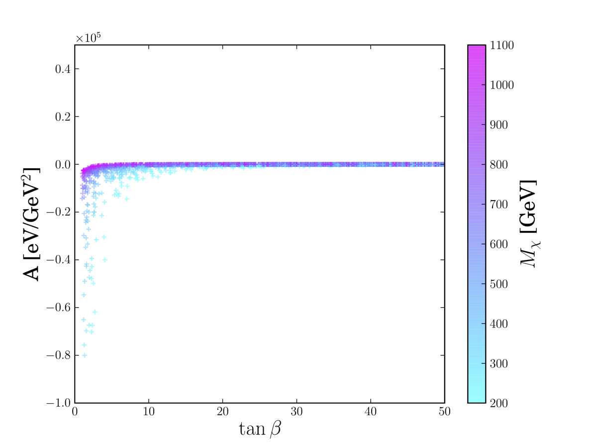
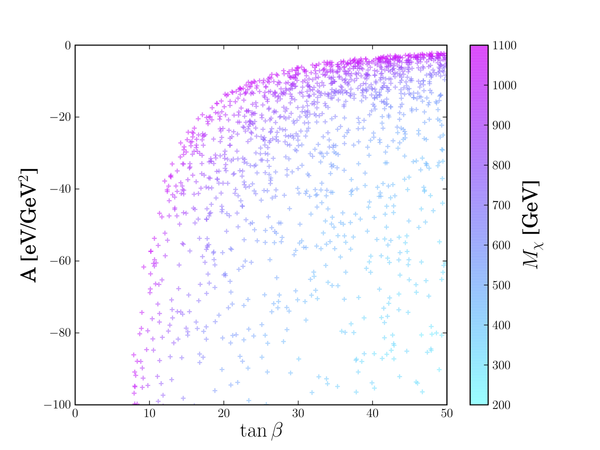
Figure 4: Coefficient $A$ as a function of $\tan\beta$ for different values of the $M_{\chi}$ scale, with a blow-up for lower values of $|A|$ in the right frame.

The value of $A$ can be directly calculated from the R-Parity conserving parameters we have been working with in the previous sections: $\tan\beta$, $\widetilde{m}$, and $M_{\chi}$, but with the addition that $\widetilde{m}$ is determined as a function of $\tan\beta$ such that we get a Higgs boson mass according to the experimental observation.

The result can be seen in fig. 4, where we have the value of $A$ as a function of $\tan\beta$ for different values of $M_{\chi}$. Both signs for $A$ are possible, obtained by switching the sign of the gaugino mass parameters. Absolute values of $A$ can be of several thousands for small values of $\tan\beta$ as well as a few units ($\mathrm{eV/GeV}^{2}$) for large $\tan\beta$ and large $M_{\chi}$. It is a characteristic of this model that the value of the Higgs mass measured at the LHC forces large values of $|A|$.

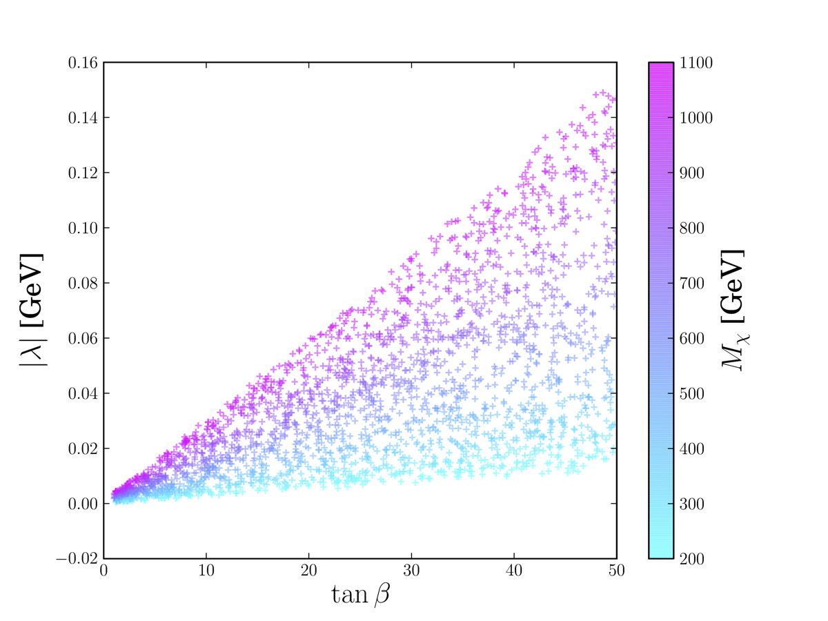
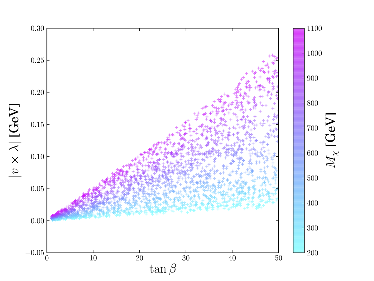
Figure 5: Values for $|\vec{\lambda}|$ (left) and $|\vec{v}\times\vec{\lambda}|$ (right) as a function of $\tan\beta$ for several different values of $M_{\chi}$.

According to eq. (14) the atmospheric mass squared difference, which experimentally is $\Delta m^{2}_{atm}\approx 2\times 10^{-3}\,{\mathrm{eV}^{2}}$, is to first order equal to $A^{2}\vec{\lambda}^{4}$, and this allow us to calculate $|\vec{\lambda}|$ in each of the scenarios defined by $\tan\beta$ and $M_{\chi}$. In fig.5-right we have $|\vec{\lambda}|$ as a function of $\tan\beta$ for different values of $M_{\chi}$. It increases with $\tan\beta$ and with $M_{\chi}$ because $A$ does the opposite. Similarly according to eq. (14) the solar mass squared difference, which experimentally satisfies $\Delta m^{2}_{sol}\approx 8\times 10^{-5}\,{\mathrm{eV}^{2}}$, is up to first order equal to $\mu_{g}^{2}{(\vec{v}\times\vec{\lambda})^{4}}/{\vec{\lambda}^{4}}$, thus we can determine $|\vec{v}\times\vec{\lambda}|$ in each of the scenarios. We see the result in fig.5-left, with a similar result compared to $|\vec{\lambda}|$, just typically twice as large.

Now we can compute the atmospheric and solar mass squared differences, which can be seen in fig. 6. We notice that, independently of the allowed value of the mass squared differences, the Higgs mass grows with $\tilde{m}$.

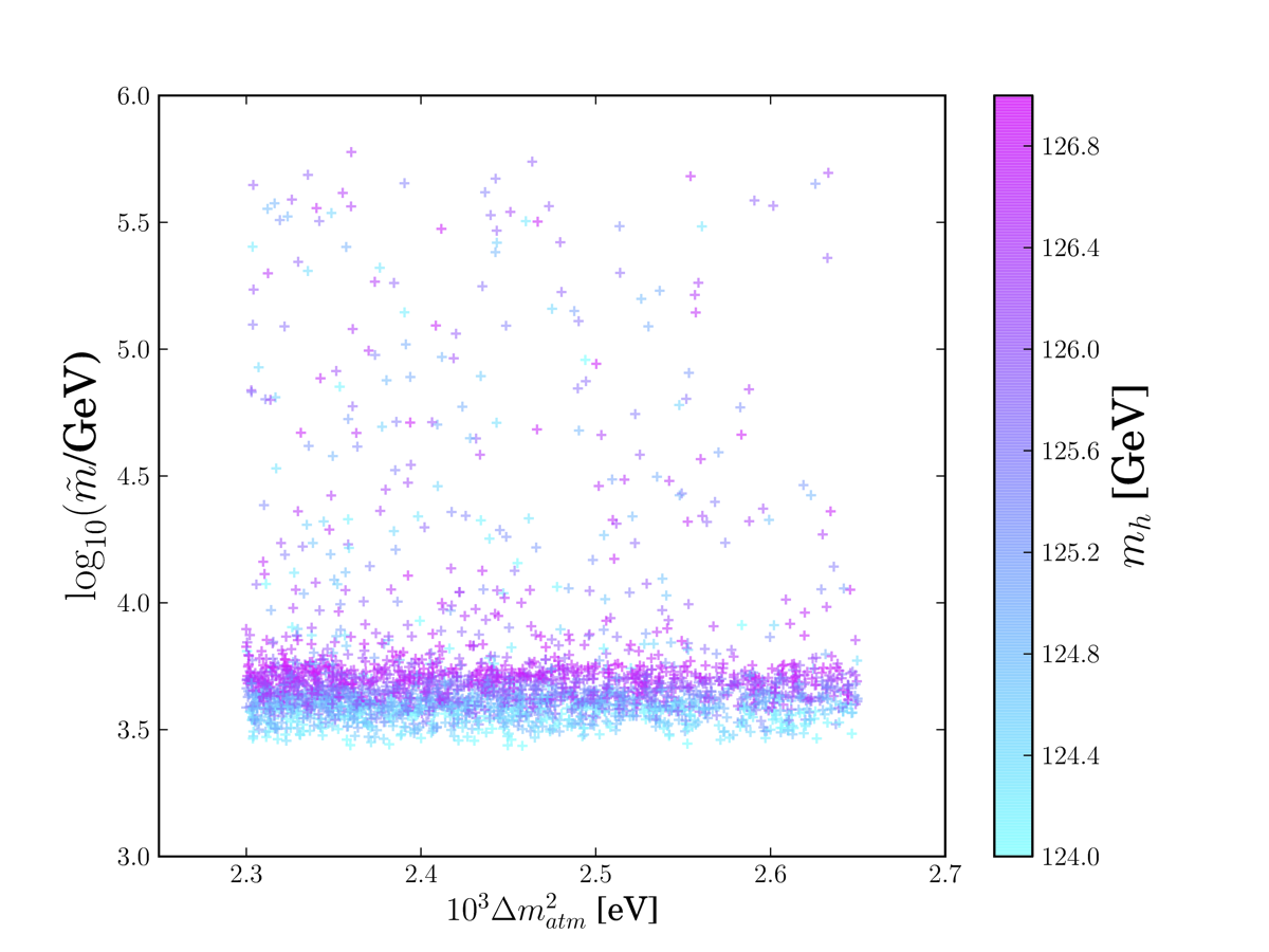
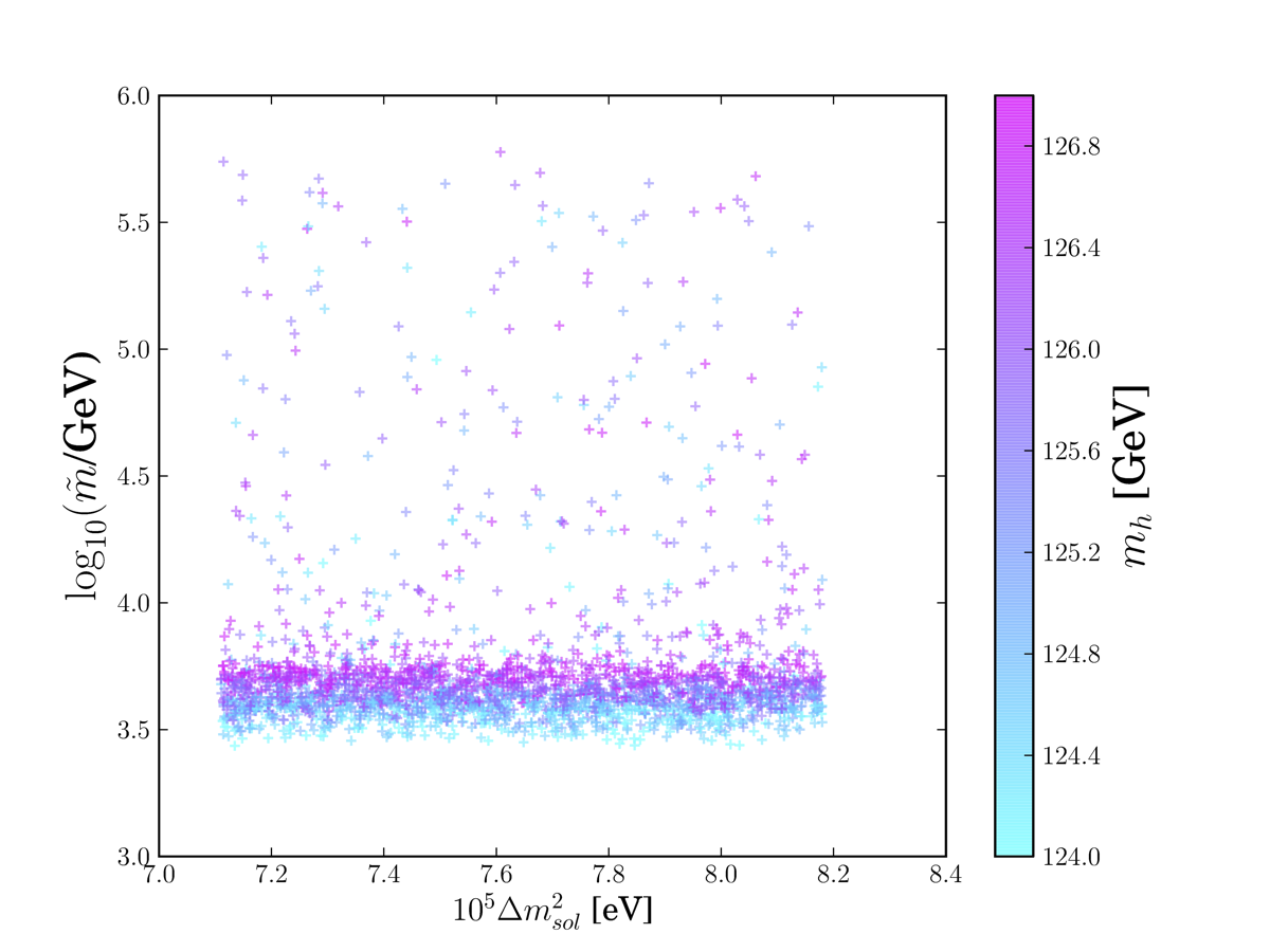
Figure 6: Values for $\Delta m^{2}_{atm}$ (left) and $\Delta m^{2}_{sol}$ (right) as a function of $\tilde{m}$ for different values of the allowed Higgs mass.

Neutrino mixing angles depend on the values of all the $\lambda_{i}$. For a diagonal charged lepton matrix, these are given by [59]

$$\sin^{2}{\theta_{reac}}=\frac{\lambda^{2}_{1}}{|\vec{\lambda}|^{2}}\hskip 5.69046pt,\hskip 5.69046pt\tan^{2}{\theta_{atm}}=\frac{\lambda^{2}_{2}}{\lambda^{2}_{1}}\hskip 5.69046pt,\hskip 5.69046pt\tan^{2}{\theta_{sol}}=\frac{(\lambda^{2}_{2}-\lambda_{1}\lambda_{2}-\lambda_{1}\lambda_{3}+\lambda^{2}_{3})^{2}}{(\lambda^{2}_{1}+\lambda^{2}_{2}+\lambda^{2}_{3})(\lambda_{3}-\lambda_{2})^{2}}.$$ (15)

On fig. 7 left we see atmospheric angle against $\tilde{m}$ for different values of our scale $M_{\chi}$. We notice that values of $\sin^{2}{\theta}_{atm}$ close to the mean $\sim 0.5$ are harder to find than the extremes in this model. This is because the Higgs mass constraint disfavors points in the parameter space where $\lambda_{1}=\lambda_{2}$, for which we have $\sin^{2}{\theta}_{atm}=\frac{1}{2}$. This can be seen on the right side of fig. 7. Notice that our scan always respects neutrino experimental values, where the criteria used is that each of the 6 observables lies within its 3$\sigma$ experimental range, and then we compute the normalized $\chi^{2}$ function with respect to the best fit, given the experimental results in [60, 61].

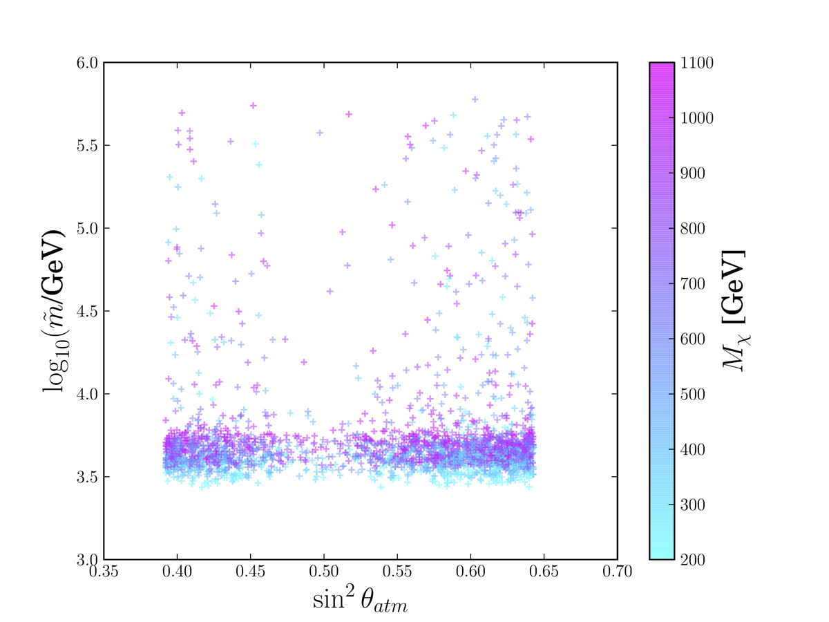
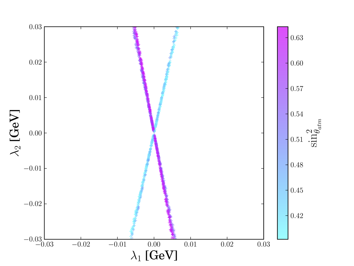
Figure 7: Values for $\sin^{2}{\theta}_{atm}$ as a function of $\tilde{m}$ for for several different values of $M_{\chi}$ (left). We also show the dependence of $\sin^{2}{\theta}_{atm}$ with the BRpV parameters $\lambda_{1}$ and $\lambda_{2}$ (right).

We show on fig. 8 the dependence of the solar and reactor angle against $\tilde{m}$ for different values of our scale $M_{\chi}$. We notice that small values of $\sin^{2}{\theta}_{reac}$ are favored, as expected in BRpV, while there is a less clear dependence for $\sin^{2}{\theta}_{sol}$.

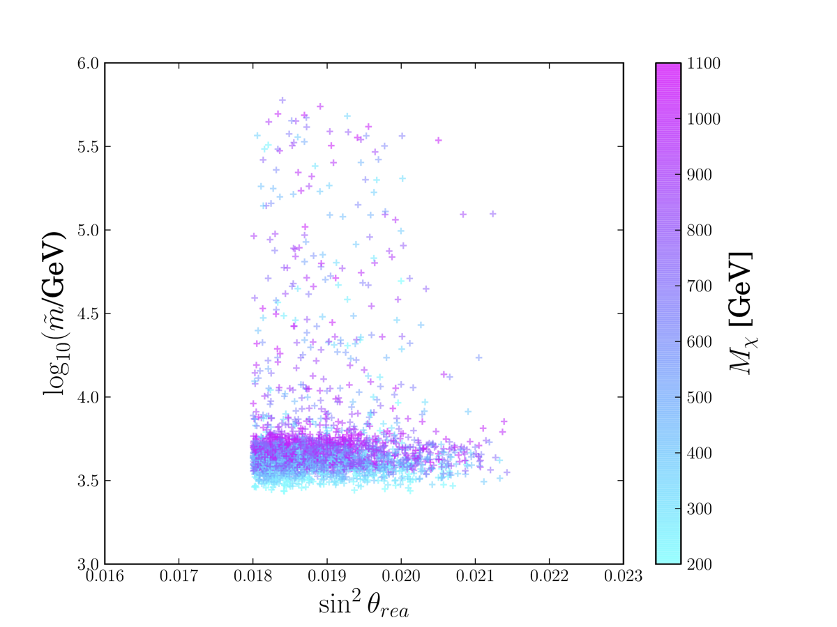
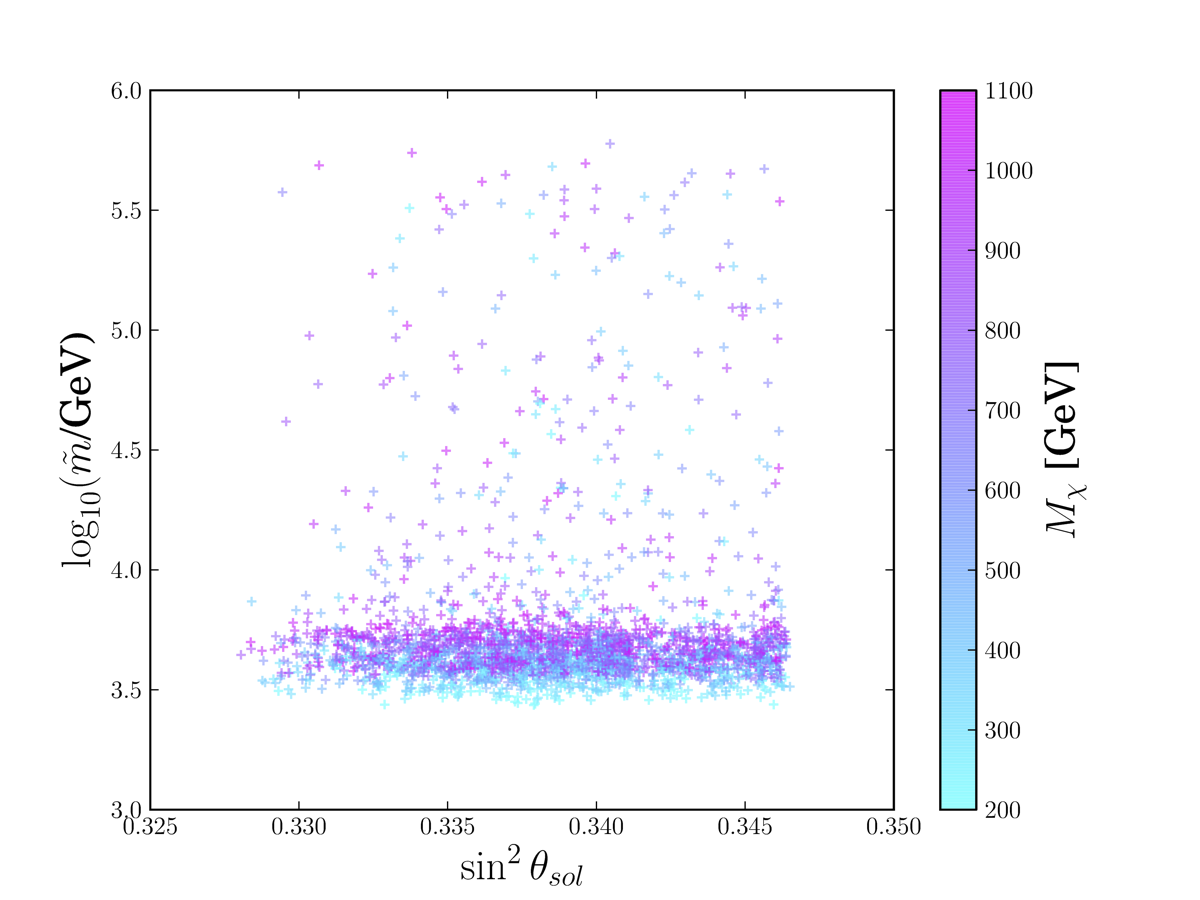
Figure 8: Values for $\sin^{2}{\theta}_{reac}$ (left) and $\sin^{2}{\theta}_{sol}$ (right) as a function of $\tilde{m}$ for several different values of $M_{\chi}$.

We also notice the heavy dependence between the solar and atmospheric angles in this model on fig. 9, quite independently of the value of $M_{\chi}$ and without fixing any of the other parameters of the model. We conclude that SS-BRpV can still deliver a good agreement with all experimental bounds.

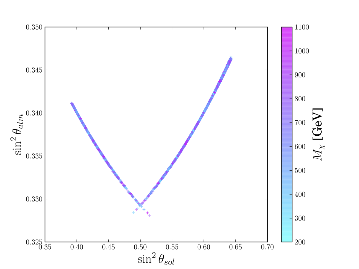
Figure 9: Allowed region in the $\sin^{2}{\theta}_{sol}$-$\sin^{2}{\theta}_{atm}$ plane for several different values of $M_{\chi}$.

4 Lightest Neutralino Decay

Another striking issue in supersymmetric models with violation of R-Parity is the instability of the lightest neutralino, which means that it is not a good candidate for Dark Matter. In these models, the gravitino is also unstable, but with a long lifetime and potentially it is a good candidate for Dark Matter [68, 67]. On the other hand, since the bilinear violation of R-parity provides an explanation for neutrino masses, the smallness of these ones implies that the RpV couplings must be relatively small, and hence, the BRpV decay rates are small. In this footing, Neutralino decay rates are related to the $\lambda_{i}$ parameters, which in turn relate these decays with the neutrino observables. If supersymmetry is realized by Nature and the lightest neutralino is observed, a precise measurement of its decay modes will be required. In the following, we study the branching ratios for the processes,

$$\chi^{0}_{1}\longrightarrow Z\nu_{\ell}\,,\qquad\chi^{0}_{1}\longrightarrow W\ell\,,\qquad\chi^{0}_{1}\longrightarrow h\nu_{\ell}$$ (16)

where $\ell$ is any of the three leptons.

Neutralino decays via sfermions are suppressed by the large sfermion masses. In Split Supersymmetry squarks and sleptons are heavy, and they are assumed to have a mass of the order $\widetilde{m}$. This scale is large, and the best approach in order to avoid large logarithms is to decouple heavy particles at that scale. Charginos and neutralinos are not necessarily as heavy, and in our approach we decouple them at a common scale $M_{\chi}\ll\widetilde{m}$. However, individual charginos and neutralinos, in practice, may have a mass different than $M_{\chi}$ depending on the actual values of the parameters $M_{1}$, $M_{2}$, and $\mu$.

In order to study the allowed parameter space for the lightest neutralino decay, we perform a general scan, by varying the free parameters of the model as indicated in table 1.

Parameter	Minimum	Maximum	Units
$\tan\beta$	$1$	$50$	-
$M_{\chi}$	$200$	$1100$	GeV
$\widetilde{m}$	$10^{4}$	$10^{10}$	GeV
$\lambda_{i}$	$-0.1$	$0.1$	GeV
$\mu_{g}$	$0.002$	$0.004$	eV

Table 1: Scanned ranges for SS-BRpV parameters.

In addition, we allow $M_{1}$, $M_{2}$, and $\mu$ to randomly vary above the decoupling scale $M_{\chi}$ according to the rule $p=M_{\chi}+rW$, where $p$ is one of these parameters, $r$ is a random number between 0 and 1, and $W$ is a window of variation that we take as $5\%$, $15\%$, $25\%$, or $50\%$ of $M_{\chi}$. For each of these windows, the lightest neutralino branching ratios are computed. In order to have consistency with the measured Higgs mass, we also impose a mass range for the SM Higgs of $124<m_{h}<127$ GeV. Furthermore, the best-fit values for neutrino oscillation physics, as given in the references [60, 61] have been used in this calculation. Under these conditions, the results for the branching ratios are shown in fig. 10.

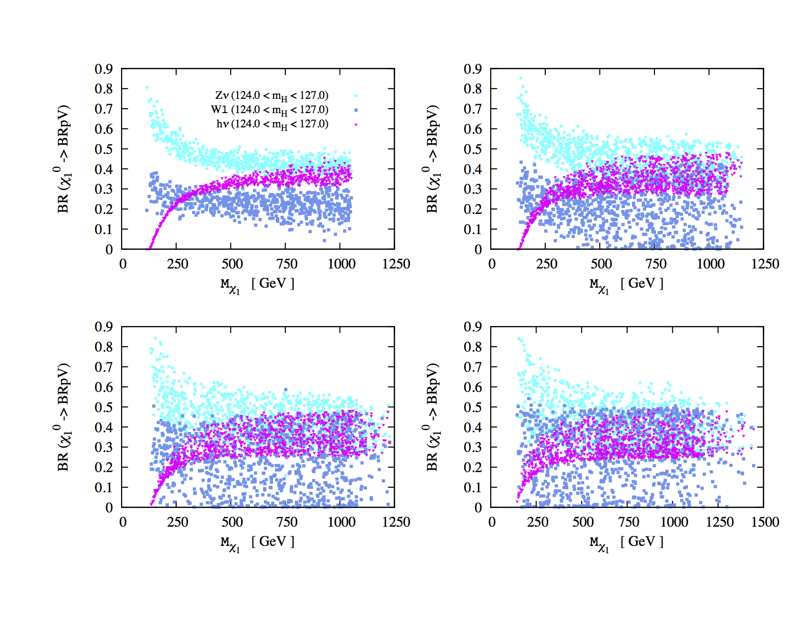
Figure 10: Branching ratios for the lightest neutralino as a function of the neutralino mass, with a decoupling scale $M_{\chi}$. Neutralino/chargino parameters $M_{1}$, $M_{2}$, and $\mu$ are allowed to vary within $5\%$ (top left), $15\%$ (top right), $25\%$ (bottom left), and $50\%$ (bottom right) of $M_{\chi}$, as explained in the text.

From the figure, we clearly see the importance of the exact spectrum of neutral and charged fermions of the model. If the neutralinos and charginos have a mass close to a common scale $M_{\chi}$, then the lightest neutralino decay via neutral particles dominates. Nonetheless, the situation is less clear if the spectrum is more spread out, and this is the case when we take an increasing window $W$ where the parameters associated to these fermions can lie. This result highlights the necessity to decouple the gauginos and higgsinos independently.

In turn, at fig. 10, we see that the channel to charged particles may become relevant when compared to the other channels insofar the $W$ window is enlarged. In order to study this channel, in fig. 11 we adopt a spread of $15\%$ and the three branching ratios $\chi^{0}_{1}\rightarrow W^{\pm}\ell^{\mp}_{i}$ for $\ell=e$, $\mu$, and $\tau$ are shown as a function of the lightest neutralino mass. We see that, for each of the points, the branching ratio $\chi^{0}_{1}\rightarrow W^{\pm}e^{\mp}$ is suppressed. This indicates that the term quadratic on $\lambda$ dominates over the $\mu_{g}$ term, since a small $BR(\chi^{0}_{1}\rightarrow W^{\pm}e^{\mp})$ is associated to a small value for the neutrino reactor angle $\theta_{13}$ [69]. The other two branching ratios can be as large as 20-30%, and any of both can be the largest.

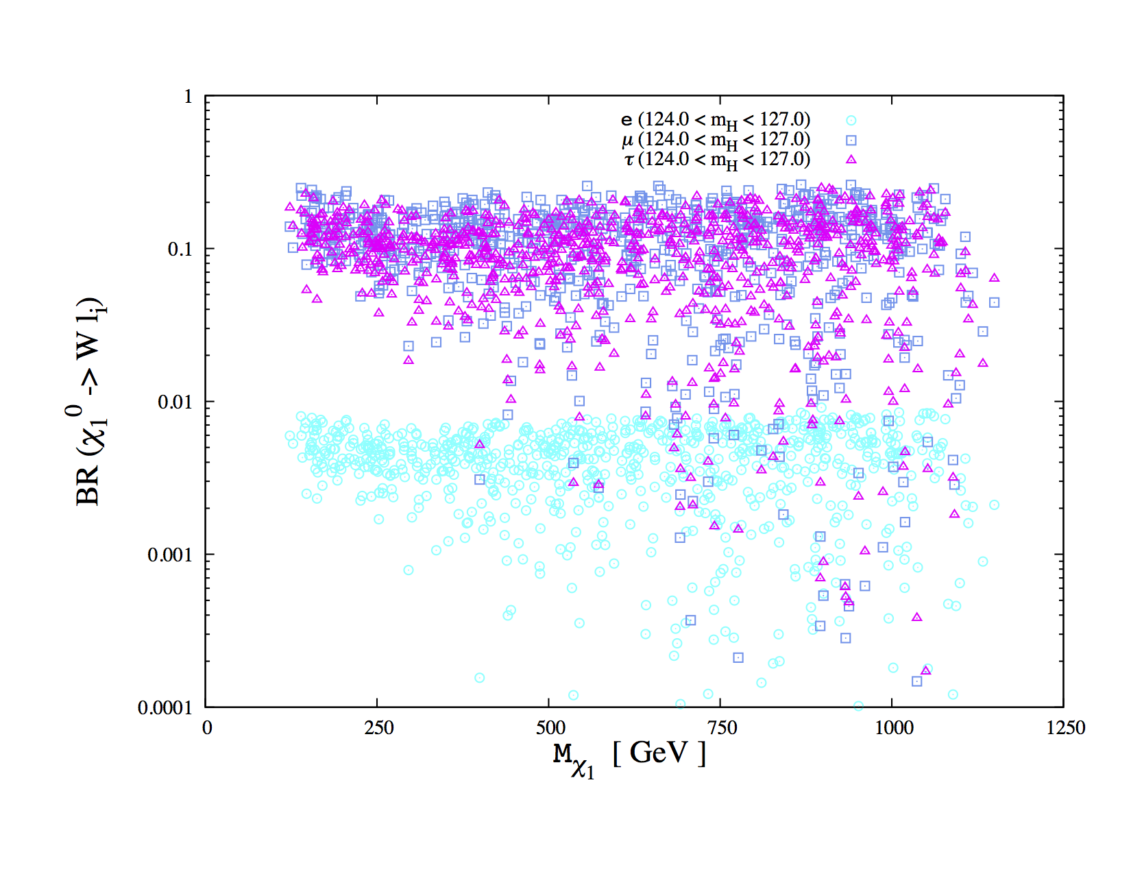
Figure 11: Branching ratios $BR(\chi^{0}_{1}\rightarrow W^{\pm}\ell^{\mp})$ as a function of the neutralino mass for the scan described in the text.

In order to have a better appreciation of the dependency of the three branching ratios we are studying, in fig. 12 we fix all the parameters with the exception of $M_{1}$, plotting the BR as a function of the neutralino mass. We choose to fix the parameters as it is indicated in table 2 within a spread of 25%. We see again that $BR(\chi^{0}_{1}\rightarrow W^{\pm}e^{\mp})$ is suppressed, and for the chosen parameters $BR(\chi^{0}_{1}\rightarrow W^{\pm}\mu^{\mp})>BR(\chi^{0}_{1}\rightarrow W^{\pm}\tau^{\mp})$, which lie between $10\%$ and $25\%$ (passing through zero) for a neutralino mass varying between 880 and 940 GeV.

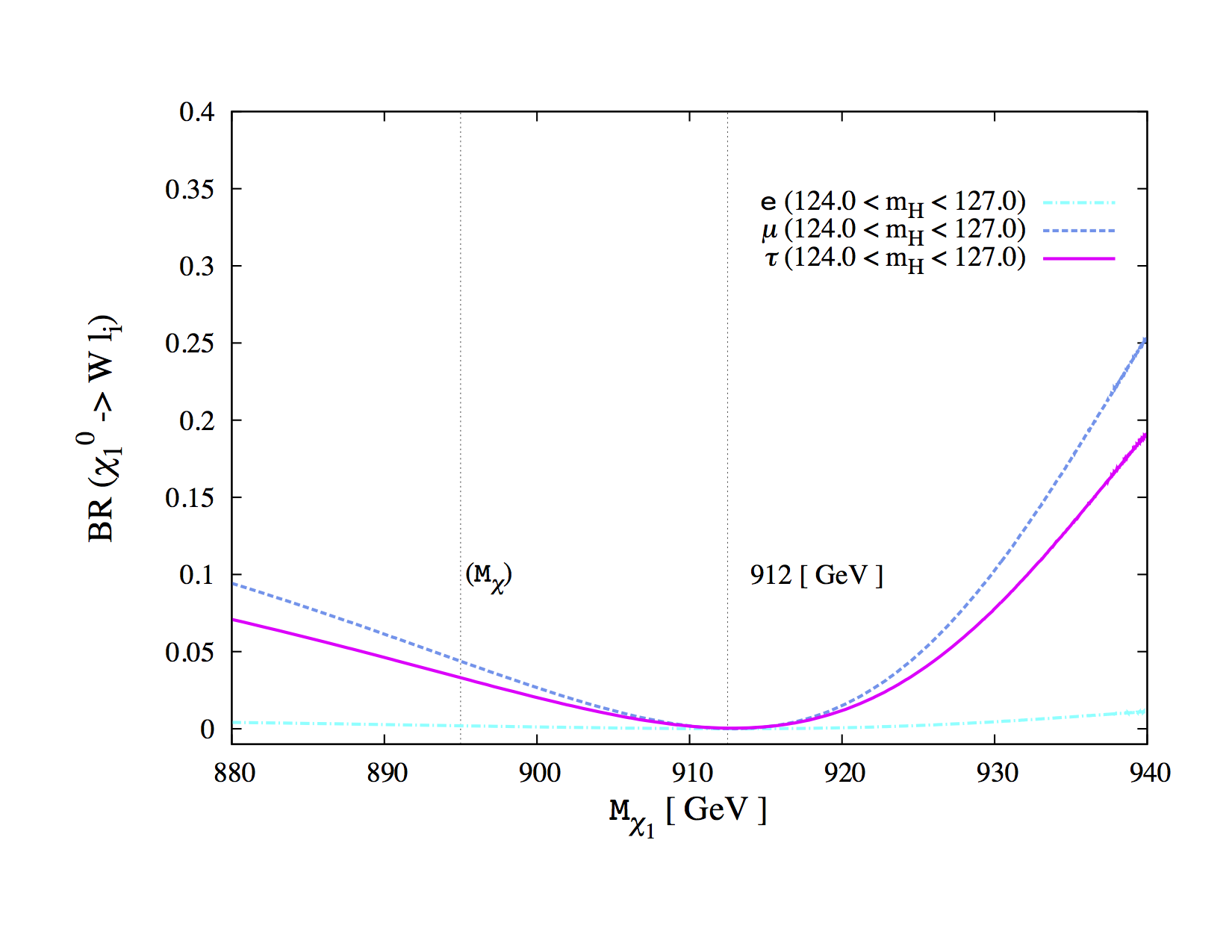
Figure 12: Branching ratios $BR(\chi^{0}_{1}\rightarrow W^{\pm}\ell^{\mp})$ as a function of the lightest neutralino mass, with parameters fixed in SS-BRpV according to table 2. The vertical dotted lines show the value for the lightest neutralino mass where the curves hit zero, at $M_{\chi_{1}}\sim 912$ GeV, and the value of the scale $M_{\chi}$.

Parameter	Value	Units
$M_{2}$	$1010$	GeV
$M_{3}$	$1500$	GeV
$\mu$	$1020$	GeV
$\tan\beta$	$2.21$	-
$M_{\chi}$	$895.31$	GeV
$\log_{10}\widetilde{m}$	$4.65$	GeV
$\lambda_{1}$	$0.00110$	GeV
$\lambda_{2}$	$0.00526$	GeV
$\lambda_{3}$	$-0.00456$	GeV
$\mu_{g}$	$0.00304$	eV

Table 2: Chosen parameters for fig. 12.

One particular feature on fig. 12, is that the three lepton branching ratios go to zero at the same value of $M_{\chi_{1}}$, in this case, around $912$ GeV. In order to understand this zero, we study the neutralino couplings to the $W$ boson. The general coupling is given by fig. 13.

$=\,i\,\gamma^{\mu}\Big{[}O^{wnc}_{Lij}\frac{(1-\gamma_{5})}{2}+O^{wnc}_{Rij}\frac{(1+\gamma_{5})}{2}\Big{]}$

Figure 13: Neutralino coupling to $W$ boson in SS-BRpV.

If we focus on $F^{0}_{i}\rightarrow\chi^{0}_{i}$ and $F^{+}_{j}\rightarrow\ell^{+}_{j}$ in the $WF^{0}F^{+}$ vertex, the couplings become $O^{wnc}_{Lij}\rightarrow O^{w\chi\ell}_{Lij}$ and $O^{wnc}_{Rij}\rightarrow O^{w\chi\ell}_{Rij}$, with

$$O^{w\chi\ell}_{Lij} = g\left[N_{i2}\xi_{L}^{j1}+\frac{1}{\sqrt{2}}N_{i3}\left(\xi_{L}^{j2}-\xi_{j3}\right)-\frac{1}{\sqrt{2}}\left(N_{i1}\xi_{j1}+N_{i2}\xi_{j2}+N_{i4}\xi_{j4}\right)\right]\equiv\widetilde{O}^{w\chi\ell}_{Lj}\lambda_{i}$$

$$O^{w\chi\ell}_{Rij} = 0$$ (17)

The quantities $N_{ij}$ are the components of the $4\times 4$ matrix that diagonalizes the neutralino sector in the neutralino-neutrino mass matrix. The quantities $\xi_{L}^{ij}$ and $\xi_{ij}$, that parametrize the chargino-charged lepton and neutralino-neutrino mixing respectively, can be found in ref. [68] and from their definition we see that the couplings in eq. (17) are proportional to the parameters $\lambda_{i}$ defined below eq. (11). If we make the following approximations: (i) motivated by the graph itself we assume the lightest neutralino is gaugino-like, (ii) we neglect the running of the $\tilde{g}$ parameters, and (iii) we assume that $v\ll M_{1}\sim M_{2}<\mu$, we obtain,

$$\widetilde{O}^{w\chi\ell}_{Lj}\approx\frac{gvc_{\beta}}{2\sqrt{2}\mu M_{2}}(g^{\prime}N_{11}+gN_{12})$$ (18)

We see that the coupling in eq. (17) is proportional to $\lambda_{i}$ and to $\widetilde{O}^{w\chi\ell}_{Lj}$. In generating fig. 12 we have kept $\lambda_{i}$ constant, thus the whole coupling of $W$ to charged fermions goes to zero at a point independent of the charged lepton because the combination $(g^{\prime}N_{11}+gN_{12})$ goes to zero. In other words, the neutralino does not couple to the $W$ gauge boson at this point. The fact that the neutralino decay mode to charged leptons may be suppressed in this model has implications on the choice of the decay mode in searches at the LHC.

5 Summary

We have studied the effect of a Higgs boson of mass $124<m_{H}<127$ GeV, motivated by measurements at the LHC, on a Split Supersymmetric model with Bilinear R-Parity Violation. We have checked that the Higgs boson mass forces the split supersymmetric scale to be rather low, $\widetilde{m}<10^{6}$ GeV, with a smaller influence from the gaugino mass. Any value of $\tan\beta$ within $1<\tan\beta<50$ is allowed, including the special case of $\tan\beta=1$, which holds possible as long as we give up gauge coupling unification, with extra new physics appearing at the scale ($>\widetilde{m}$) where the top Yukawa coupling becomes non-perturbative.

We constrain neutrino parameters in this model, given the experimental results on neutrino observables and Higgs mass. We find that independently of the allowed value of the mass squared differences, the Higgs mass grows with $\tilde{m}$ and rather small values of $\tilde{m}$ are preferred, given the Higgs mass constrain. We also notice the effects of imposing a Higgs mass constrain in the neutrino mixing angles. We find a striking dependence between the solar and atmospheric angles in this model, where strong constrains on $\sin^{2}{\theta}_{sol}$ limits $\sin^{2}{\theta}_{atm}$ quite independently of the chargino/neutralino decoupling scale. We still find points in the allowed parameter space in good agreement with all experimental bounds.

Finally, we have studied the two-body decays of the lightest neutralino in detail, in particular, the effects of the exact spectrum of neutralinos and charginos and their decoupling. In general, the neutralino branching ratios are dominated by the channel to neutral particles, but insofar the exact spectrum is more spread around a larger decoupling scale, there may be other hierarchies for the neutralino branching ratios where the channel to charged particles may be more relevant. This issue indicates that the decoupling of charginos and neutralinos should be performed taking into account their exact spectrum. In addition, we conclude that future decaying neutralino searches at the LHC in this model should focus first on decays to neutral fermions.

References

- [1] G. Aad et al. [ATLAS Collaboration], Phys. Lett. B 716, 1 (2012) [arXiv:1207.7214 [hep-ex]].
- [2] G. Aad et al. [ATLAS Collaboration], Phys. Rev. D 90, no. 5, 052004 (2014) [arXiv:1406.3827 [hep-ex]].
- [3] S. Chatrchyan et al. [CMS Collaboration], JHEP 1306, 081 (2013) [arXiv:1303.4571 [hep-ex]].
- [4] S. Chatrchyan et al. [CMS Collaboration], Phys. Lett. B 716, 30 (2012) [arXiv:1207.7235 [hep-ex]].
- [5] F. Englert and R. Brout, Phys. Rev. Lett. 13, 321 (1964).
- [6] P. W. Higgs, Phys. Rev. Lett. 13, 508 (1964).
- [7] P. W. Higgs, Phys. Lett. 12, 132 (1964).
- [8] G. S. Guralnik, C. R. Hagen and T. W. B. Kibble, Phys. Rev. Lett. 13, 585 (1964).
- [9] P. W. Higgs, Phys. Rev. 145, 1156 (1966).
- [10] T. W. B. Kibble, Phys. Rev. 155, 1554 (1967).
- [11] S. L. Glashow, Nucl. Phys. 22, 579 (1961).
- [12] S. Weinberg, Phys. Rev. Lett. 19, 1264 (1967).
- [13] A. Salam, Conf. Proc. C 680519, 367 (1968).
- [14] G. ’t Hooft and M. J. G. Veltman, Nucl. Phys. B 44, 189 (1972).
- [15] G. Aad et al. [ATLAS Collaboration], JHEP 1409, 176 (2014) [arXiv:1405.7875 [hep-ex]].
- [16] G. Aad et al. [ATLAS Collaboration], arXiv:1501.03555 [hep-ex].
- [17] G. Aad et al. [ATLAS Collaboration], arXiv:1501.01325 [hep-ex].
- [18] G. Aad et al. [ATLAS Collaboration], JHEP 1406, 124 (2014) [arXiv:1403.4853 [hep-ex]].
- [19] S. Chatrchyan et al. [CMS Collaboration], Eur. Phys. J. C 73, no. 12, 2677 (2013) [arXiv:1308.1586 [hep-ex]].
- [20] S. Chatrchyan et al. [CMS Collaboration], Phys. Rev. Lett. 112, 161802 (2014) [arXiv:1312.3310 [hep-ex]].
- [21] G. Aad et al. [ATLAS Collaboration], JHEP 1310, 130 (2013) [Erratum-ibid. 1401, 109 (2014)] [arXiv:1308.1841 [hep-ex]].
- [22] V. Khachatryan et al. [CMS Collaboration], arXiv:1502.04358 [hep-ex].
- [23] N. Arkani-Hamed and S. Dimopoulos, JHEP 0506, 073 (2005) [hep-th/0405159].
- [24] G. F. Giudice and A. Romanino, Nucl. Phys. B 699, 65 (2004) [Erratum-ibid. B 706, 65 (2005)] [hep-ph/0406088].
- [25] V. D. Barger, C. Kao and R. J. Zhang, Phys. Lett. B 483, 184 (2000) [hep-ph/9911510];
- [26] H. Baer, P. Mercadante and X. Tata, Phys. Lett. B 475, 289 (2000) [hep-ph/9912494].
- [27] A. Arbey, M. Battaglia, A. Djouadi, F. Mahmoudi and J. Quevillon, Phys. Lett. B 708, 162 (2012) [arXiv:1112.3028 [hep-ph]];
- [28] L. J. Hall, Y. Nomura and S. Shirai, JHEP 1406, 137 (2014) [arXiv:1403.8138 [hep-ph]].
- [29] P. Gambino, G. F. Giudice and P. Slavich, Nucl. Phys. B 726, 35 (2005) [hep-ph/0506214].
- [30] V. Khachatryan et al. [CMS Collaboration], arXiv:1501.05603 [hep-ex].
- [31] G. Aad et al. [ATLAS Collaboration], JHEP 1501, 068 (2015) [arXiv:1411.6795 [hep-ex]].
- [32] G. Aad et al. [ATLAS Collaboration], JHEP 1409, 176 (2014) [arXiv:1405.7875 [hep-ex]].
- [33] G. Aad et al. [ATLAS Collaboration], arXiv:1504.05162 [hep-ex].
- [34] S. Chatrchyan et al. [CMS Collaboration], Phys. Lett. B 733, 328 (2014) [arXiv:1311.4937 [hep-ex]].
- [35] W. Kilian, T. Plehn, P. Richardson and E. Schmidt, Eur. Phys. J. C 39, 229 (2005) [hep-ph/0408088].
- [36] J. L. Hewett, B. Lillie, M. Masip and T. G. Rizzo, JHEP 0409, 070 (2004) [hep-ph/0408248].
- [37] S. Jung and J. D. Wells, Phys. Rev. D 89, no. 7, 075004 (2014) [arXiv:1312.1802 [hep-ph]].
- [38] D. S. M. Alves, E. Izaguirre and J. G. Wacker, arXiv:1108.3390 [hep-ph].
- [39] F. Wang, W. Wang, F. q. Xu, J. M. Yang and H. Zhang, Eur. Phys. J. C 51, 713 (2007) [hep-ph/0612273].
- [40] S. K. Gupta, P. Konar and B. Mukhopadhyaya, Phys. Lett. B 606, 384 (2005) [hep-ph/0408296].
- [41] K. Cheung and W. Y. Keung, Phys. Rev. D 71, 015015 (2005) [hep-ph/0408335].
- [42] H. K. Dreiner, M. Hanussek and S. Grab, Phys. Rev. D 82, 055027 (2010) [arXiv:1005.3309 [hep-ph]].
- [43] M. Hirsch, M. A. Diaz, W. Porod, J. C. Romao and J. W. F. Valle, Phys. Rev. D 62, 113008 (2000) [Erratum-ibid. D 65, 119901 (2002)] [hep-ph/0004115].
- [44] M. A. Diaz, J. C. Romao and J. W. F. Valle, Nucl. Phys. B 524, 23 (1998) [hep-ph/9706315].
- [45] R. Hempfling, Nucl. Phys. B 478, 3 (1996) [hep-ph/9511288].
- [46] B. de Carlos and P. L. White, Phys. Rev. D 54, 3427 (1996) [hep-ph/9602381].
- [47] P. Nath and P. Fileviez Perez, Phys. Rept. 441, 191 (2007) [hep-ph/0601023].
- [48] A. Choudhury and A. Datta, JHEP 1206, 006 (2012) [arXiv:1203.4106 [hep-ph]].
- [49] H. Baer, V. Barger and A. Mustafayev, JHEP 1205, 091 (2012) [arXiv:1202.4038 [hep-ph]].
- [50] W. Buchmuller, L. Covi, K. Hamaguchi, A. Ibarra and T. Yanagida, JHEP 0703, 037 (2007) [hep-ph/0702184 [HEP-PH]].
- [51] S. Bailly, K. -Y. Choi, K. Jedamzik and L. Roszkowski, JHEP 0905, 103 (2009) [arXiv:0903.3974 [hep-ph]].
- [52] D. Restrepo, M. Taoso, J. W. F. Valle and O. Zapata, Phys. Rev. D 85, 023523 (2012) [arXiv:1109.0512 [hep-ph]].
- [53] M. Aguilar et al. [AMS Collaboration], Phys. Rev. Lett. 110, 141102 (2013).
- [54] E. Carquin, M. A. Diaz, G. A. Gomez-Vargas, B. Panes and N. Viaux, arXiv:1501.05932 [hep-ph].
- [55] D. Hooper, P. Blasi and P. D. Serpico, JCAP 0901, 025 (2009) [arXiv:0810.1527 [astro-ph]].
- [56] G. F. Giudice and A. Strumia, Nucl. Phys. B 858, 63 (2012) [arXiv:1108.6077 [hep-ph]].
- [57] N. Arkani-Hamed, A. Gupta, D. E. Kaplan, N. Weiner and T. Zorawski, arXiv:1212.6971 [hep-ph].
- [58] A. Arvanitaki, N. Craig, S. Dimopoulos and G. Villadoro, JHEP 1302, 126 (2013) [arXiv:1210.0555 [hep-ph]].
- [59] M. A. Diaz, B. Koch and B. Panes, Phys. Rev. D 79, 113009 (2009) [arXiv:0902.1720 [hep-ph]].
- [60] D. V. Forero, M. Tortola and J. W. F. Valle, Phys. Rev. D 86, 073012 (2012) [arXiv:1205.4018 [hep-ph]].
- [61] D. V. Forero, M. Tortola and J. W. F. Valle, Phys. Rev. D 90, no. 9, 093006 (2014) [arXiv:1405.7540 [hep-ph]].
- [62] N. Bernal, A. Djouadi and P. Slavich, JHEP 0707, 016 (2007) [arXiv:0705.1496 [hep-ph]].
- [63] A. Hoecker, Nucl. Phys. Proc. Suppl. 218, 189 (2011) [arXiv:1012.0055 [hep-ph]].
- [64] K. Nakamura et al. [Particle Data Group Collaboration], J. Phys. G G 37, 075021 (2010).
- [65] M. A. Diaz, P. Fileviez Perez and C. Mora, Phys. Rev. D 79, 013005 (2009) [hep-ph/0605285].
- [66] E. J. Chun, D. W. Jung, S. K. Kang and J. D. Park, J. Korean Phys. Soc. 45, S278 (2004) [hep-ph/0312329].
- [67] M. A. Diaz, S. G. Saenz and B. Koch, Phys. Rev. D 84, 055007 (2011) [arXiv:1106.0308 [hep-ph]].
- [68] G. Cottin, M. A. Diaz, M. J. Guzman and B. Panes, Eur. Phys. J. C 74, no. 11, 3138 (2014) [arXiv:1406.2368 [hep-ph]].
- [69] X. Guo et al. [Daya-Bay Collaboration], hep-ex/0701029.