Extrema statistics in the dynamics of a non-Gaussian random field

Abstract

When the equations that govern the dynamics of a random field are nonlinear, the field can develop with time non-Gaussian statistics even if its initial condition is Gaussian. Here, we provide a general framework for calculating the effect of the underlying nonlinear dynamics on the relative densities of maxima and minima of the field. Using this simple geometrical probe, we can identify the size of the non-Gaussian contributions in the random field, or alternatively the magnitude of the nonlinear terms in the underlying equations of motion. We demonstrate our approach by applying it to an initially Gaussian field that evolves according to the deterministic KPZ equation, which models surface growth and shock dynamics.

Random fields that undergo a time evolution according to a nonlinear dynamical equation often develop non-Gaussian statistics that provide clues about the details of the underlying microscopic mechanisms. Consider for example a gas-liquid phase transition. In the early stages, there are many randomly small volumes in which all the molecules are in the same phase, distributed randomly. Over time, these volumes will grow and merge, thereby gradually replacing the Gaussian disorder with structure cite_Bray.

Even if the initial condition of a random field is Gaussian, the dynamics will typically generate a non-Gaussian component in the field that we wish to quantify and track with time. The standard approach to detect and measure non-Gaussianities is to employ higher-order correlation functions. In this work, we adopt a geometric approach to measuring the non-Gaussian component of a scalar field $h(\vec{r},t)$: we interpret it as a height function describing an evolving surface, and study its geometry. Gaussian surfaces have certain general geometric and topological properties cite_Dennis1; cite_Longuet2; cite_Berry; cite_Longuet1; cite_Dennis2. For example, the number of maxima exactly balances the number of minima. A random surface that does not exhibit this property is then guaranteed to have non-Gaussian statistics cite_paper1; cite_paper2.

In previous articles cite_paper1; cite_paper2 we studied fields that are local functions of a given Gaussian, i.e. of the form $h(\vec{r})=H(\vec{r})+f_{NL}(H(\vec{r}))$, where $H$ is a Gaussian field and $f_{NL}$ a nonlinear function. In this scheme, the perturbed height $h$ at any point $\vec{r}$ is a function only of the original height $H(\vec{r})$ at the same point. In this paper, we move to the general case of nonlocal perturbations, which e.g. include a dependence on $\nabla H$, thereby introducing a mixing between the field values at different points.

Such a nonlocal non-Gaussianity can arise in a broad range of physical contexts, for example as the result of nonlinear diffusion. For concreteness, consider a diffusion equation of the general form

$$\frac{\partial h(\vec{r},t)}{\partial t}=D\nabla^{2}h(\vec{r},t)+f_{NL}(h,\nabla h),$$ (1)

where $f_{NL}$ is any nonlinear function. If we let $h$ be a Gaussian field at $t=0$, then non-Gaussianities will emerge as a consequence of the last term; if we would omit this term, we retrieve the heat equation, which would preserve the Gaussianity of $h$ for all $t>0$. A variety of known diffusion equations has this general form. For instance, when $f_{NL}$ takes the form $-h^{2}$ we get Fisher’s equation, which can be used as a model to describe the growth and saturation of a population. Another example is the Cahn-Hilliard equation for the development of order after a phase transition cite_Bray. Several models of structure formation, in both condensed matter cite_Chaikin and cosmology cite_Dodelson, also belong to this class.

To illustrate our general result, we apply it to the case of a field obeying the deterministic KPZ equation cite_KPZ, for which $f_{NL}=\frac{\lambda}{2}(\nabla h)^{2}$. This equation is often used to model the height profile of a growing surface. A field that starts out as a Gaussian field will acquire non-Gaussian characteristics as time progresses. We use our formula to quantify the resulting effect on the relative difference in densities of maxima and minima. This allows to back up the non-Gaussian component in $h$, or alternatively, to deduce what the nonlinear coefficient $\lambda$ is. We verify the analytical predictions by comparing them with results from computer simulations.

The outline of this paper is as follows. In section I we determine a general expression for the imbalance between maxima and minima for a non-Gaussian field. This is applied to the KPZ equation in section II. Finally, section LABEL:sec_conclusions summarizes our conclusions.

I Non-Gaussian fields

A homogeneous and isotropic Gaussian field is defined in terms of its Fourier components as

$$H(\vec{r})=\sum_{\vec{k}}A(k)\cos(\vec{k}\cdot\vec{r}+\phi_{\vec{k}}).$$ (2)

The phases $\phi_{\vec{k}}$ are independent random variables, uniformly distributed between $0$ and $2\pi$. The amplitude spectrum $A(k)$ depends only on the magnitude of the wave vector $\vec{k}$ and encodes the special features of the Gaussian field under consideration. An alternative approach is to express the amplitude spectrum in terms of its moments, according to

$$K_{n}=\sum_{\vec{k}}\tfrac{1}{2}A(k)^{2}k^{n}.$$ (3)

For convenience, we will consider $H$ to be normalized, such that $K_{0}=\langle H^{2}\rangle=1$, see ref. cite_paper1 for more details.

In what follows, we concentrate on homogeneous and isotropic fields $h(\vec{r})$, which we assume to be in the form of a Gaussian $H(\vec{r})$ with the addition of a perturbation. Unlike refs. cite_paper1; cite_paper2, we will not restrict ourselves to a perturbation of the local kind, i.e. where the perturbation at any point $\vec{r}$ is a function of $H(\vec{r})$ only. We will now also accommodate perturbations which depend on $\vec{\nabla}H$ for instance, or evolve over time. Such perturbations introduce a mixing between the values of the field at different points, which we will designate as nonlocal perturbations.

We will investigate the effect of a perturbation on the densities of maxima and minima. A maximum (minimum) $\vec{r_{0}}$ of $h$ is defined by the condition $h_{x}(\vec{r_{0}})=h_{y}(\vec{r_{0}})=0$, along with the inequalities $h_{xx}(\vec{r_{0}})h_{yy}(\vec{r_{0}})-h_{xy}(\vec{r_{0}})^{2}>0$ (if this were negative, $\vec{r_{0}}$ would be a saddle point) and $h_{xx}(\vec{r_{0}})$, $h_{yy}(\vec{r_{0}})$ negative (positive); note that the first condition implies that $h_{xx}(\vec{r_{0}})$ and $h_{yy}(\vec{r_{0}})$ have the same sign. The $x$ and $y$ subscripts indicate derivatives with respect to the coordinates of the two-dimensional plane.

The general procedure that we use is very similar to the one in cite_paper2 and is as follows: we consider a fixed point $\vec{r_{0}}$ – due to the homogeneity of $h$, the analysis will not depend on this choice. We determine the joint probability distribution of $h_{x}$, $h_{y}$, $h_{xx}$, $h_{yy}$ and $h_{xy}$, since these stochastic variables are the ingredients from which maxima and minima are defined, as outlined above. This distribution can be determined via the generating function, which in turn can be constructed by determining the relevant cumulants involving the five stochastic variables. Once the probability distribution is obtained, we set $h_{x}=h_{y}=0$ and integrate the second derivatives over the region defining a minimum (maximum) in order to get the density of minima (maxima).

As we did in cite_paper2, we transform to another coordinate system, based on the complex coordinates $z=x+iy$ and $z^{*}$, which will allow us to make full use of the homogeneity and isotropy of $h$ later on. In this new basis, we have

$$\frac{\partial}{\partial z} =\tfrac{1}{2}\frac{\partial}{\partial x}-\tfrac{1}{2}i\frac{\partial}{\partial y} \frac{\partial}{\partial z^{*}} =\tfrac{1}{2}\frac{\partial}{\partial x}+\tfrac{1}{2}i\frac{\partial}{\partial y}.$$ (4)

In this coordinate system, the definition of a maximum (minimum) becomes $h_{z}(\vec{r_{0}})=0$, $|h_{zz^{*}}(\vec{r_{0}})|>|h_{zz}(\vec{r_{0}})|$ and $h_{zz^{*}}(\vec{r_{0}})$ is negative (positive).

Some care is required however, since we are now dealing with complex variables $h_{z}$ and $h_{zz}$ ($h_{zz^{*}}$ is real). We will treat the variables $z$ and $z^{*}$ as if they were independent. Therefore, next to $h_{z}$, we will consider $h_{z^{*}}$ as well, as a separate random variable, although it is actually the complex conjugate of $h_{z}$. Similarly, we also include $h_{z^{*}z^{*}}=h_{zz}^{*}$. Therefore, we are still dealing with five variables: $h_{z}$, $h_{zz}$, their conjugates, and $h_{zz^{*}}$.

As stated before, we will arrive at the joint probability distribution of these variables by building the generating function, which is the Fourier transform of the probability distribution. For a set of $n$ correlated variables $\xi_{i}$ this is

$$\begin{split}&\chi(\lambda_{1},\ldots,\lambda_{n})\\ &\qquad=\int\!\mathrm{d}\xi_{1}\ldots\mathrm{d}\xi_{n}\,p(\xi_{1},\ldots,\xi_{n})e^{i(\xi_{1}\lambda_{1}+\ldots+\xi_{n}\lambda_{n})}.\end{split}$$ (5)

By expanding the exponential into a Taylor series we find that the coefficients – which are called the moments of the distribution (not to be confused with the moments from eq. (3)) – are correlations: rLl & 2l χ(λ_1, …, λ_n)
  = 1 + i ∑_j ⟨ξ_j ⟩λ_j + i22! ∑_j_1,j_2 ⟨ξ_j_1ξ_j_2 ⟩λ_j_1λ_j_2
+  i33! ∑_j_1,j_2,j_3 ⟨ξ_j_1ξ_j_2ξ_j_3 ⟩λ_j_1λ_j_2λ_j_3 + … If we do the same for the logarithm of $\chi$, we obtain the cumulants:

$$\log\chi=\> i\sum_{j}C_{1}(\xi_{j})\lambda_{j}+\frac{i^{2}}{2!}\sum_{j_{1},j_{2}}C_{2}(\xi_{j_{1}},\xi_{j_{2}})\lambda_{j_{1}}\lambda_{j_{2}}$$

$$+\frac{i^{3}}{3!}\sum_{j_{1},j_{2},j_{3}}C_{3}(\xi_{j_{1}},\xi_{j_{2}},\xi_{j_{3}})\lambda_{j_{1}}\lambda_{j_{2}}\lambda_{j_{3}}+\ldots$$ (6)

From eqs. (5) and  (6) it can be derived that the cumulants can be factorized into moments, for example

$$\begin{split}C_{3}(\xi_{1},\xi_{2},\xi_{3})=\>&\langle\xi_{1}\xi_{2}\xi_{3}\rangle-\langle\xi_{1}\rangle\langle\xi_{2}\xi_{3}\rangle-\langle\xi_{2}\rangle\langle\xi_{3}\xi_{1}\rangle\\ &-\langle\xi_{3}\rangle\langle\xi_{1}\xi_{2}\rangle+2\langle\xi_{1}\rangle\langle\xi_{2}\rangle\langle\xi_{3}\rangle.\end{split}$$ (7)

If all the cumulants are known, one can reconstruct the generating function and from that obtain the probability distribution via an inverse Fourier transformation.

The defining characteristic of Gaussian variables is that all cumulants are zero, apart from the second order ones ($C_{2}$). If $h$ were a Gaussian field, then this would apply to $p(h_{z},h_{zz},h_{zz^{*}})$, since the derivatives of a Gaussian field are themselves also Gaussian fields. Since $h$ is non-Gaussian, this is not the case. The first-order cumulants are still zero; for instance, we have $C(h_{z})=\langle h_{z}\rangle=\partial_{z}\langle h\rangle=0$ since $\langle h\rangle$ is constant due to the homogeneity of $h$. The third-order cumulants are however nonzero. We will include these and see how they influence the probability distribution and the densities of maxima and minima.

In principle, there are infinitely many nonzero cumulants. However, a field that is generated by a nonlinear differential equation, like eq. (1), typically has small cumulants of high order. In particular, if $f_{NL}$ is a quadratic function and the initial conditions are Gaussian, then the $n$-th order cumulants scale like $f_{NL}^{n-2}$ (for $n>2$) – see appendix LABEL:app_cumulants. Therefore we will only need to determine cumulants up to third order to get the correction to leading order.

The usefulness of the complex variables $z$ and $z^{*}$ becomes apparent when we look for all nonzero cumulants of second and third order involving the five variables we have. Since $h$ is isotropic, a moment like $\langle h_{z^{*}}h_{zz}\rangle$ should not change when we rotate the field by an arbitrary angle $\alpha$. Such a rotation would give $z\rightarrow e^{i\alpha}z$ and $z^{*}\rightarrow e^{-i\alpha}z^{*}$. Incorporating these in the derivatives causes the aforementioned moment to pick up a factor $e^{i\alpha}$. Since we argued that the moment should not be affected by the rotation, it must be zero. In general, any moment involving a different number of $z$ and $z^{*}$ derivatives is zero by this argument. Since cumulants can be decomposed into moments, as depicted in eq. (7), the same applies to cumulants.

Furthermore, translational symmetry implies some relations between the cumulants. From translational invariance it follows that any correlation should be constant with respect to $\vec{r}$. For instance, using the product rule, we have

$$0=\partial_{z^{*}}\langle h_{z}^{2}h_{z^{*}}\rangle=\langle h_{z}^{2}h_{z^{*}z^{*}}\rangle+2\langle h_{z}h_{z^{*}}h_{zz^{*}}\rangle,$$ (8)

which gives us the relation present in eq. (9c).

Therefore, there are only a few independent cumulants that are (potentially) nonzero:

$$\sigma =\langle|h_{z}|^{2}\rangle,$$ (9a)

$$\alpha =\langle|h_{zz}|^{2}\rangle=\langle h_{zz^{*}}^{2}\rangle,$$ (9b)

$$\beta =\langle|h_{z}^{2}|h_{zz^{*}}\rangle=-\tfrac{1}{2}\langle h_{z}^{2}h_{z^{*}z^{*}}\rangle=-\tfrac{1}{2}\langle h_{z^{*}}^{2}h_{zz}\rangle,$$ (9c)

$$\gamma =\langle h_{zz^{*}}^{3}\rangle,$$ (9d)

$$\delta =\langle|h_{zz}|^{2}h_{zz^{*}}\rangle.$$ (9e)

In these definitions, the cumulants have been expanded into moments in accordance with eq. (7); since the first-order correlations are zero, as noted before, only the third-order correlations remain. We also introduced the shorthand notation $|h_{z}|^{2}=h_{z}h_{z}^{*}=h_{z}h_{z^{*}}$ and similarly for $|h_{zz}|^{2}$. Note also that the third-order cumulants, $\beta$, $\gamma$ and $\delta$ are close to zero when $h$ is close to being Gaussian, which we assume. On the other hand, $\sigma$ and $\alpha$ are nonzero in general.

We can now construct the logarithm of the generating function as prescribed by eq. (6),

$$\begin{split}\log\chi=&-\sigma|\lambda_{z}|^{2}-\alpha|\lambda_{zz}|^{2}-\tfrac{1}{2}\alpha\lambda_{zz^{*}}^{2}\\ &-i\beta|\lambda_{z}|^{2}\lambda_{zz^{*}}+i\beta(\lambda_{z}^{2}\lambda_{z^{*}z^{*}}+\lambda_{z^{*}}^{2}\lambda_{zz})\\ &-\tfrac{i}{6}\gamma\lambda_{zz^{*}}^{3}-i\delta|\lambda_{zz}|^{2}\lambda_{zz^{*}}.\end{split}$$ (10)

Note that some cumulants appear multiple times in eq. (6) since the $\lambda$’s can be permuted (if they are not all the same); this explains why for instance the term $\lambda_{zz^{*}}^{3}$ has a prefactor $i/6$ whereas the prefactor of $|\lambda_{zz}|^{2}\lambda_{zz^{*}}=\lambda_{zz}\lambda_{z^{*}z^{*}}\lambda_{zz^{*}}$ is $i$ (due to the 6 distinct permutations of the $\lambda$’s).

We see that $\chi$ features an exponential of a third-degree polynomial, making the inverse Fourier transform – to be performed in order to get the probability distribution – nontrivial. Remember however that the cubic terms are small owing to the near-Gaussianity of $h$, allowing us to make the expansion

$$\begin{split}\chi=\>&\Big{[}1-i\beta|\lambda_{z}|^{2}\lambda_{zz^{*}}+i\beta(\lambda_{z}^{2}\lambda_{z^{*}z^{*}}+\lambda_{z^{*}}^{2}\lambda_{zz})\\ &\quad-\tfrac{i}{6}\gamma\lambda_{zz^{*}}^{3}-i\delta|\lambda_{zz}|^{2}\lambda_{zz^{*}}\Big{]}\\ &\times\exp\big{(}\!-\!\sigma|\lambda_{z}|^{2}-\alpha|\lambda_{zz}|^{2}-\tfrac{1}{2}\alpha\lambda_{zz^{*}}^{2}\big{)}.\end{split}$$ (11)

The inverse Fourier transform of this gives rll 3l p(h_z, h_zz, h_zz^*)
 =  & [ 1 + βασ2h_zz^*(|h_z|^2 - σ) - βασ2(h_z^2h_z^*z^* + h_z^*^2h_zz)
+ γ6α3(h_zz^*^3 - 3αh_zz^*) + δα3h_zz^*(|h_zz|^2-α) ]
2l ×1π22πσα3/2 e^-|h_z|^2/σ- |h_zz|^2/α- h_zz^*^2/2α.

Now that the joint probability distribution of the relevant derivatives is obtained, we can set $h_{z}=h_{z^{*}}=0$ – this condition defines a critical point. The joint probability distribution measures how likely it is that $h_{z}$ and $h_{z^{*}}$ are close to zero for a certain point $\vec{r}$. What is needed however is for $h_{z}$ and $h_{z^{*}}$ to be exactly zero for a point close to $\vec{r}$, since we are looking for a density with respect to the $(x,y)$-plane. For this, we need to go from a probability density with respect to $h_{z}$ and $h_{z^{*}}$ to one with respect to $z$ and $z^{*}$ (representing $x$ and $y$). This is accomplished by multiplying $p$ with the following Jacobian:

$$J=\bigg{|}\frac{\partial(h_{z},h_{z^{*}})}{\partial(z,z^{*})}\bigg{|}=\big{|}|h_{zz}|^{2}-h_{zz^{*}}^{2}\big{|}.$$ (12)

Now we are ready to set $h_{z}=h_{z^{*}}=0$ and integrate $pJ$ over $h_{zz}$ and $h_{zz^{*}}$. The range is determined by the type of critical point of interest; focus on the minima first. For these we must have $|h_{zz}|<|h_{zz^{*}}|$ and $h_{zz^{*}}>0$. The integration over $h_{zz}$ is done by integrating over its real and imaginary part. Since the integrand depends only on the modulus of $h_{zz}$, we move to polar coordinates. Let us define $r=|h_{zz}|$ and $s=h_{zz^{*}}$. The integration range is then $0<r<s$, and with eq. (2) we get rll & 2l n_min = 1π22πσα3/2
 ×∫_0^∞​ ds ∫_0^s ​ 2πr   dr   (s^2 - r^2) e^-r^2/α- s^2/2α
×[1 - βασ s + γ6α3 (s^3-3αs) + δα3 s(r^2-α) ]. This integration is pretty straightforward: although the range of $r$ is finite, the integrand is a Gaussian multiplied by a polynomial that has only odd degrees of $r$, hence it does not give rise to error functions. The resulting integral over $s$ is also standard. The final result reads

$$n_{min}=\frac{\alpha}{2\sqrt{3}\pi\sigma}-\frac{1}{\pi\sigma}\sqrt{\frac{\alpha}{2\pi}}\Big{(}\frac{4}{3}\frac{\beta}{\sigma}+\frac{4}{9}\frac{\delta}{\alpha}-\frac{10}{27}\frac{\gamma}{\alpha}\Big{)}.$$ (13)

For a Gaussian field, we would have $\beta=\gamma=\delta=0$, $\sigma=\frac{1}{4}K_{2}$ and $\alpha=\frac{1}{16}K_{4}$. This would give us $n_{min}=K_{4}/(8\sqrt{3}\pi K_{2})$, exactly as given in cite_Longuet2.

To get the density of maxima, the same integrand as in eq. (I) needs to be integrated over the range $s<0$ and $0<r<-s$. However, note that if we make the transformation $s\rightarrow-s$, the range of integration is the same as in eq. (I). Furthermore, note that the transformation $s\rightarrow-s$ in the integrand is equivalent to $\beta\rightarrow-\beta$, $\gamma\rightarrow-\gamma$ and $\delta\rightarrow-\delta$. With this insight, we easily find that the expression for $n_{max}$ is the same as the above, except with a plus in place of the first minus.

With this result, the imbalance between maxima and minima is found to be

$$\Delta n\equiv\frac{n_{max}-n_{min}}{n_{max}+n_{min}}=\sqrt{\frac{6}{\pi\alpha}}\bigg{(}\frac{4}{3}\frac{\beta}{\sigma}+\frac{4}{9}\frac{\delta}{\alpha}-\frac{10}{27}\frac{\gamma}{\alpha}\bigg{)}.$$ (14)

This is the main result of this paper. As an illustration, we shall now use this result to understand the evolution of maxima and minima in the context of a differential equation describing surface growth.

II KPZ equation

The deterministic Kardar-Parisi-Zhang (KPZ) equation cite_KPZ is given by

$$\frac{\partial h}{\partial t}=\nu\nabla^{2}h+\frac{\lambda}{2}(\nabla h)^{2}.$$ (15)

This equation is often used to describe the height profile of a growing surface: the first term on the right-hand side describes the diffusion of particles along the surface, while the second term accounts for the assumption that the growth is perpendicular to the slope of the surface, while $h$ describes the height along the universal up direction cite_Barabasi. This leads to (see fig. 1)

$$\frac{\mathrm{d}h}{\mathrm{d}t}=\lambda\sqrt{1+(\nabla h)^{2}}=\lambda+\frac{\lambda}{2}(\nabla h)^{2}+\ldots$$ (16)

The leading term $\lambda$ is ignored since it is just a constant that does not affect the profile of the surface.

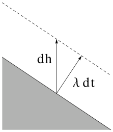
Figure 1: A geometrical interpretation of the KPZ equation applied to a growing surface. The surface is assumed to grow perpendicularly at a constant rate $\lambda$. Measured vertically, the growth rate is $\mathrm{d}h/\mathrm{d}t\approx\lambda(1+\frac{1}{2}(\nabla h)^{2})$.

Another interpretation of eq. (15) is obtained by taking the gradient on both sides, which yields

$$\frac{\partial\vec{v}}{\partial t}=\nu\nabla^{2}\vec{v}+\lambda\vec{v}\vec{\nabla}\vec{v},$$ (17)

where $\vec{v}=\vec{\nabla}h$ is a velocity field. This is a vector Burger’s equation which arises in fluid mechanics. The maxima and minima of $h$ correspond to sources and sinks of $v$.

We will take $h(\vec{r},t)$ to be a Gaussian field at $t=0$, and use our result eq. (14) to determine how the non-Gaussianities, which arise and evolve due to the KPZ equation, influence the densities of maxima and minima.

First note that if we would set $\lambda=0$ in eq. (15), we retrieve the heat equation, which preserves the Gaussianity of a field: if we enter $h(\vec{r},t=0)=H(\vec{r})$, where $H(\vec{r})$ is a Gaussian field as given by eq. (2), we find that the solution is

$$h(\vec{r},t)=\sum_{\vec{k}}A(k)e^{-k^{2}\nu t}\cos(\vec{k}\cdot\vec{r}+\phi_{k}).$$ (18)

We find that the amplitudes pick up a factor $\exp(-k^{2}\nu t)$, but the phases remain independent. Therefore, even though its amplitude spectrum changes, $h(\vec{r},t)$ remains Gaussian at any time $t$ and the density of maxima and minima remains the same, since this is a general property of Gaussian fields.

If we have $\lambda\neq 0$, $h(\vec{r},t)$ no longer remains Gaussian. In fact, as we will see, the density of maxima and minima is no longer the same. We shall assume $\lambda$ to be small in comparison with $\nu$, and find out how these densities differ as a function of time, using eq. (14). For this, we need to determine the two- and three-point correlations $\sigma$, $\alpha$, $\beta$, $\gamma$ and $\delta$.

First, we substitute $u=\exp((\lambda/2\nu)h)$. Note that, since this is a monotonically increasing function of $h$, the maxima and minima of $u$ are exactly the same points as those of $h$. In terms of $u$, the KPZ equation becomes:

$$\frac{\partial u}{\partial t}=\nu\nabla^{2}u,$$ (19)

which is simply the heat equation. However, $u(\vec{r},t=0)=\exp((\lambda/2\nu)h_{0})$ is now not a Gaussian field. If we assume that $\lambda\ll\nu$, we have:

$$u_{0}=1+\frac{\lambda}{2\nu}h_{0}+\frac{\lambda^{2}}{8\nu^{2}}h_{0}^{2}+O((\lambda/\nu)^{3}).$$ (20)

Since the leading term, equal to one, has no influence on either the maxima and minima or the heat equation, we can ignore it. The same applies to the prefactor $\frac{\lambda}{2\nu}$ of the second term. Hence we make a final transformation

$$v\equiv\frac{2\nu}{\lambda}(u-1),$$ (21)

$$v_{0}=h_{0}+\frac{\lambda}{4\nu}h_{0}^{2}+O((\lambda/\nu)^{2}).$$ (22)

Note that $v$ still obeys the heat equation and also shares the same maxima and minima with $h$ and $u$. Moreover, we now have $v(\vec{r},t=0)$ in the desired form of a Gaussian $h_{0}$ plus a perturbation. Since $v$ obeys the heat equation, we can use the corresponding Green’s function to write down the general solution

$$v(r,t) =\int\mathrm{d}^{2}\tilde{r}\,G(r,\tilde{r},t)v_{0}(\tilde{r})$$

$$=\int\mathrm{d}^{2}\tilde{r}\,\frac{1}{4\pi\nu t}e^{-\frac{(r-\tilde{r})^{2}}{4\nu t}}\big{(}h_{0}(\tilde{r})+\frac{\lambda}{4\nu}h_{0}(\tilde{r})^{2}\big{)},$$ (23)

where $v_{0}(\tilde{r})=v(r,t=0)$.

We can now calculate the five correlations needed to determine $\Delta n$. We will demonstrate the procedure using $\sigma=\langle v_{z}(r,t)v_{z^{*}}(r,t)\rangle$ as an example. rLl σ& 2L = ⟨v_z(r,t) v_z^*(r,t) ⟩
= ∬ d^2 ~r_1 d^2 ~r_2   ∂_z_1 G(r_1,~r_1,t)
∂_z^*_2 G(r_2,~r_2,t) ⟨v