Symmetry in Self-Similarity in Space and Time—Short Time Transients and Power-Law Spatial Asymptote

Abstract

The self-similarity in space and time (hereafter self-similarity), either deterministic or statistical, is characterized by similarity exponents and a function of scaled variable, called the scaling function. In the present paper, we address mainly the self-similarity in the limit of early stage, as opposed to the latter one, and also consider the scaling functions that decay or grow algebraically, as opposed to the rapidly decaying functions such as Gaussian or error function. In particular, in the case of simple diffusion, our symmetry analysis shows a mathematical mechanism by which the rapidly decaying scaling functions are generated by other polynomial scaling functions. While the former is adapted to the self-similarity in the late-stage processes, the latter is adapted to the early stages. This paper sheds some light on the internal structure of the family of self-similarities generated by a simple diffusion equation. Then, we present an example of self-similarity for the late stage whose scaling function has power-law tail, and also several cases of self-similarity for the early stages. These examples show the utility of self-similarity to a wider range of phenomena other than the late stage behaviors with rapidly decaying scaling functions.

I Introduction

When the evolution of state shows some scaling behavior involving both space and time without fixed characteristic length or time, it is said to have self-similarity in space and time (hereafter, “self-similarity” for short) [1]. Self-similarity is a symmetry of the time-dependent fields which remain invariant under certain scale transformations of space and time. Similarity and dimensional methods in mechanics has long been known ([2] and references therein). Dynamical critical phenomena [3] or the late-stage dynamics of the first-order transition [4] are among the typical examples that have been studied a lot. Deterministic cases have also been actively studied (e.g., see the book [1]). The  self-similarity is represented by some scaled variables, scaling exponents, and scaling functions. Among the simplest examples of self-similarity is the smearing Gaussian distribution governed by a diffusion equation, where the diffusing field $\phi$ evolves, for example, in the form $\phi(x,t)=t^{-\alpha}f(xt^{-{\frac{1}{2}}}),$ where $f(s)=\exp(-\mbox{const.}\times s^{2})$ is the scaling function for the scaled variable, $xt^{-{\frac{1}{2}}},$ and $\alpha$ is the scaling exponent, being $1/2$ in this case. Such symmetry object, scaling function, can have different types, and one of our main goals is to relate the scaling functions of different types.

Thus far, most studies on the self-similarity in physics have focused on the late-stage evolution, i.e., well after the initial transient, and at the same time focused on the case where the scaling function or its derivative decays rapidly, i.e., faster than any power-law as a function of the scaled variable. The basic reason for this is the fact that the group velocity in the parabolic or hyperbolic evolution equation is vanishing or finite at large length scale. This implies that the self-similarity with algebraic asymptotes of the scaling function is reduced to static (with steady flux) algebraic tails in the far field. As such far field condition has been rarely prepared physically, we have not paid much attention to the self-similarity with power-low asymptotes in the scaling function.

Self-similarity does not exclusively occur in the late stage, where the spatial scale is also large. Self-similarity as the short-time limit has not drawn much attention thus far, to the authors’ knowledge. In this limit, the local region is infinitely magnified by the scaled variable. Then, the scaling functions are not constrained to decay rapidly but they can even grow algebraically for large values of scaled variable.

In this paper, we first analyze the internal symmetry properties in the family of scaling functions for the 1D diffusion system (Section II). Through the equation governing the scaling function and its adjoint equation together with the operator of “Wick rotation”, the scaling functions with rapidly decaying asymptote, which are suitable for the late-stage self-similarity, are related to the polynomial scaling functions, suitable for the short-time self-similarity. Secondly, we present some examples of self-similarity having the scaling functions with algebraic asymptote (Section III): The first example is the late-stage self-similarity having an algebraically decaying scaling function which we think to be realizable in the permeative relaxation process of hydrogel. The other examples are the short-time self-similarity of 1D diffusion from parabolic or cusp-like initial field configuration and the short-time self-similarity of 1D linearized capillary-driven thin-film equation. Through these studies, we shed light on the family of self-similarity behaviors and the relationship among them. In  Section IV, we briefly discuss the generalizability of the results obtained in this paper.

II Symmetry Properties in the Family of Scaling Functions for the 1D Diffusion Process

II.1 Scaling Functions

For the 1D diffusion, $\partial u/\partial t=\partial^{2}u/\partial x^{2},$ different approaches have been developed (see, for example, [5]). Here, we focus on the solutions with self-similarity in space and time.

$${u(x,t)=u_{p}(x,t)\equiv{t^{-{\,(p+1)}/{2}}}\phi_{p}({t^{-1/{2}}{x}}),}$$ (1)

where the scaling function $\phi_{p}(s)$ should obey

$${\mathcal{L}_{p}\,\phi_{p}(s)=0,\mbox{with}\mathcal{L}_{p}=\frac{d^{2}}{ds^{2}}+\frac{s}{2}\frac{d}{ds}+\frac{p+1}{2}.}$$ (2)

The index $p$ has been adjusted so that $p=0$ corresponds to the Gaussian scaling function. The even and odd solutions, $\Phi_{p}^{\rm(even)}(s)$ and $\Phi_{p}^{\rm(odd)}(s),$ respectively, are given in Appendix A with some explicit form for several $p$ values. Here, we note only those properties that are relevant for the discussion below: For non-integer values of $p$, the solution behaves asymptotically with power law, $|\phi_{p}(s)|\sim|s|^{-(p+1)},$ for $|s|\to\infty.$ The special cases are: (i) the solutions with rapidly decaying derivatives for non-negative integer $p$ with even [odd] parities when p is even [odd]; and (ii) the polynomial solutions for negative integer $p$ with even [odd] parities when p is odd [even]. Surprisingly, (i) and (ii) are related to each other, as shown below. For the diffusion equation or heat equation, the general similarity solutions have been studied in detail (see, for example, [6]). However, the focus has not been put on the relationship among the solutions.

II.2 Symmetry in the Family of Scaling Functions

We noticed the two independent ways to relate the operators $\mathcal{L}_{p}$ defined by Equation (2) for $p\in{\mathbb{R}}$ and their adjoint ones, $\mathcal{L}^{\dagger}_{p}$, defined by

$${\mathcal{L}_{p}^{\dagger}=\frac{d^{2}}{ds^{2}}-\frac{1}{2}\frac{d}{ds}s+\frac{p+1}{2}.}$$ (3)

The first relation between $\mathcal{L}_{p}$ and $\mathcal{L}^{\dagger}_{p}$ is nothing but the definition of adjoint, i.e., the “integration by parts” identity,

$$\psi_{p}(s)\mathcal{L}_{p}\phi_{p}(s)-\phi_{p}(s)\mathcal{L}_{p}^{\dagger}\psi_{p}(s)=\frac{d}{ds}{\left[{\psi_{p}^{\prime}(s)\phi_{p}(s)-\psi_{p}(s)\phi_{p}^{\prime}(s)-\frac{s}{2}\psi_{p}(s)\phi_{p}(s)}\right]}.$$ (4)

Equation (4) means that $\phi_{p}$ satisfying $\mathcal{L}_{p}\phi_{p}=0$ and $\psi_{p}$ satisfying $\mathcal{L}^{\dagger}_{p}\psi_{p}(s)=0$ are mutually the integrating factor of the other. In fact, if we have such $\psi_{p},$ the solution of $\mathcal{L}_{p}\phi_{p}=0$ can be constituted from the vanishing condition of the right-hand side of Equation (4). The latter condition leads to

$$\phi_{p}(s)=C_{1}\,\psi_{p}(s)e^{-\frac{s^{2}}{4}}+C_{2}\int^{s}_{1}\frac{\psi_{p}(s)}{[\psi_{p}(u)]^{2}}e^{-\frac{s^{2}}{4}+\frac{u^{2}}{4}}du,$$ (5)

where $C_{1}$ and $C_{2}$ are the integration constants, and the integration pathway is assumed to be properly chosen to avoid the poles of the integrand. The second relation between $\mathcal{L}_{p}$ and $\mathcal{L}^{\dagger}_{p}$ is through a kind of Wick rotation:

$${{\mathcal{L}}_{p}\circ J=-J\circ\mathcal{L}^{\dagger}_{q},\qquad p+q+1=0,}$$ (6)

where the operator $J$ is defined such that $J\circ\Phi(s)=\Phi(is)$ for any object including $s$ as a variable. The identity in Equation (6) can be verified by elementary calculus.

The presence of two different pathways connecting the family $\{\phi_{p}\}$ with that of $\{\psi_{q}\}$ reveals the intra-relationship among the scaling functions $\{\phi_{p}\}$, which is mediated by $\{\psi_{q}\}.$ Figure 1 schematically shows this mechanism:

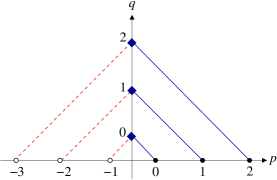
Figure 1: Diagram showing the relations among the solutions of $\mathcal{L}_{p}$ and those of $\mathcal{L}^{\dagger}_{q}.$ See the main text.

A solution of $\mathcal{L}_{p}\phi_{p}=0$ (e.g., $p=-3$) gives the solution of $\mathcal{L}^{\dagger}_{q}\psi_{q}=0$ with $p+q+1=0$ (e.g., $q=+2$) through $\phi_{p}(s)=\psi_{q}(is).$ Once $\psi_{q}(s)$ satisfying $\mathcal{L}^{\dagger}_{q}\psi_{q}=0$ is given, the solution of $\mathcal{L}_{p}\phi_{p}(s)=0$ with $p=q$ (e.g., $p=2$) is constructed by Equation (5) with $\psi_{p}(s)$ and $\psi_{p}(u)$ being replaced by $\phi_{-(p+1)}(-is)$ and $\phi_{-(p+1)}(-iu),$ respectively.

While the above symmetry property applies for any real index $p$, the cases of particular interest are when $\phi_{-p-1}(s)$ are polynomial with non-negative integers $p.$ Such $\phi_{-p-1}(s)$ can generate, through $\psi_{p}$, the $\phi_{p}(s)$ whose derivative decays rapidly as the term $\propto C_{1}$ in Equation (5). Such polynomial solution $\phi_{-p-1}(s)$ has its origin in the adjoint equation $\mathcal{L}^{\dagger}_{p}\psi_{p}=0,$ which can in turn be reduced to the Hermite equation by changing variable, $y=s/2.$ This type of analysis may shed some light on the internal structure of the family of dynamical similarities of a system of evolution, although for the moment being limited to a particular case. In Section III.2, we study the case where $\phi_{-p-1}$ is $\Phi_{-3,e}$ or $\Phi_{-2,o}$ as short-time self-similar evolution. The above-mentioned symmetry connects these scaling functions to the rapidly decaying ones $\Phi_{2,e}$ and $\Phi_{1,o}$ in the notation used in Appendix A.

III Self-Similarity in Space and Time with Scaling Function Having Algebraic Tail

As mentioned above, we should realize that, when the scaling function of self-similarity has algebraic tails as function of the scaled variable, these algebraic asymptotes must be realized in the initial field configuration. For example, in Equation (2) for the 1D diffusion equation, the algebraic tail issues from the last two terms in $\mathcal{L}_{p},$ whose balance implies $\partial u/\partial t\simeq 0.$ Indeed, if we put $\sim|s|^{-(p+1)}$ for $\phi_{p}(s)$ in Equation (1), we have $u_{p}(x,t)\sim t^{0}\,x^{-(p+1)}.$ This consequence is intuitively understandable because most of the evolution system of our interest spreads mainly locally, being unable to update substantially the configurations far apart. Below, we present some examples of self-similarity having algebraic spatial tail. One is for the late stage and the other two are for the short-time limit.

III.1 Late-Stage Self-Similarity in Space and Time of Gel Network

It is generally difficult to prepare an algebraic static asymptotes over a large spatial range. This may be the reason the self-similarity having algebraic tails has been scarcely studied in physical application. Below, we present an example that an algebraic tail is nevertheless thinkable. The system considered is an aqueous gel, i.e., a soft solid consisting of a very fine permeable network saturated with water. Such a system responds as if it were an incompressible isotropic elastic body at short-time scale while its permeative relaxation under an osmotic pressure gradient is very slow. As the setup, we suppose a uniform 3D aqueous gel having a small water-filled hole around the center, $r=0.$ The hole’s radius is $R_{0}.$ For $t<0$, the gel is in uniform equilibrium under no stress and, at $t=0$, we quickly inject a small amount of water into the hole. The injection makes expand the holes from radius $R_{0}$ to $R_{1}(>R_{0}).$ Soon after the injection, a quick elastic re-equilibration without permeation will take place, where each material point on the gel network has been pushed off radially. We denote by $U_{\rm rad}(r,0^{+})$ the initial radial displacement of the material point which has been at the radius $r.$ This displacement must satisfy $4\pi r^{2}U_{\rm rad}(r,0^{+})=({4\pi}/3)[R_{1}^{3}-R_{0}^{3}]$ because the gel network behaves incompressible at short timescale (where we assume $|U_{\rm rad}|\ll R_{0}$). Thus, we can prepare an algebraic initial configuration, $U_{\rm rad}(r,0^{+})\propto r^{-2},$ which is exact in the limit of for $r/R_{0}\to\infty.$ The subsequent very slow permeative relaxation obeys the standard elasto-hydrodynamic model [7], which gives the following time evolution equation for the radial displacement field $U_{\rm rad}(r,t)$:

$${{\left({\frac{\partial}{\partial t}-D{\left[{\frac{\partial^{2}}{\partial r^{2}}-\frac{2}{r^{2}}}\right]}}\right)}[r\,U_{\rm rad}(r,t)]=0,}$$ (7)

where $D$ is the (cooperative) diffusion constant $D=(K+4\mu/3)/f,$ with $f$, $\mu$, and $K$ being, respectively, the permeative friction coefficient between the gel network and solvent, the shear modulus, and the bulk (osmotic) modulus of the gel [8]. Hereafter, we use the units such that $D=1.$ In the late-stage, $\sqrt{t}\gg R_{0},$ at large distance $r\gg R_{0},$ Equation (7) allows the similarity solutions of the form, $U_{\rm rad}(r,t)=U^{(r)}_{p}(r,t)\equiv{t^{-{(p+1)}/{2}}}\Psi_{p}{\left({{r}/{\sqrt{t}}}\right)},$ where $p=1$ is compatible with our initial condition. See Appendix B for the details including the analytical solutions. Figure 2 shows the evolution of self-similarity solution, $U_{1}^{\rm(r)}(r,t)=t^{-1}\Psi_{1}(r/\sqrt{t}),$ at $t=1,4$ and $9.$ We see there that the algebraic tail of the radial displacement at large $r$ remains unchanged until the time $t\sim r^{2}.$

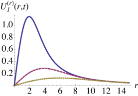
Figure 2: Radial displacement of the gel. The radial displacement, $U_{\rm rad}(r,t)=U_{1}^{(r)}(r,t)\equiv t^{-1}\Psi_{1}(r/\sqrt{t}),$ is shown vs. $r$ for the various time, $t=1$ (blue), $4$ (magenta), and $9$ (yellow). The vertical scale has been arbitrarily chosen and $R_{0}$ is supposed to be infinitesimal. For $r\gg\sqrt{t}$, the displacement, ${U_{1}^{(r)}}(r,t),$ retains a time-independent tail, $\sim r^{-2}.$ While the finiteness of $R_{0}$ should modify the radial displacements at small scale, $r\sim R_{0},$ it does not influence the fate of the algebraic tail.

III.2 Self-Similarity in Space and Time in the Short-Time Limit of 1D Diffusion

Parabolic or wedge-shaped apexes are among the most generic local configurations that we encounter as the initial conditions of diffusion. While the former is generic form around the smooth extrema, the latter should be realized when some spatially localized source is removed after having established the wedge-shaped steady state profile. We discuss the simple case of one-dimension, but the generalization to higher dimensions is straightforward. In Figure 3a,b, the parabolic and wedge-like initial conditions are shown by solid curves, respectively. Their functional forms are $u(x,0)=\max(1-x^{2},0)$ and $u(x,0)={\max}[1-|x|,0]$.

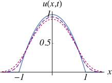
(a)

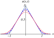
(b)

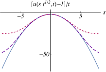
(c)

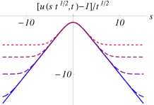
(d)

Figure 3: (a,b) Initial conditions (solid curves) as well as the short-time evolution at $t=0.02$ and $t=0.04$ (dashed curves in (a)) and at $t=0.005,0.01,$ and $0.02$ (dashed curves in (b)), respectively, are shown versus the unscaled variables. The initial condition has $u(0,0)=1$ and the support, $[-1,1].$ (c,d) The scaling function and the short-time evolution are represented using the scaled variables: (c) replots the evolution in (a) using $[u(x,t)-u(0,0)]/t$ and $s=x/\sqrt{t}$ and compares with $\phi_{-3}(s)=2+s^{2},$ while (d) replots the evolution in (b) using $[u(x,t)-u(0,0)]/\sqrt{t}$ with $s$ and compares with $\phi_{-2}(s)=e^{-{s^{2}}/{4}}+({\sqrt{\pi}\,s}/{2}){\rm erf}({s}/{2}).$

The time evolution in the early stage is also shown in the same figure. In Figure 3c,d, the same evolutions are replotted by the scaled variables. In both cases, parabolic or wedge-like apexes, we can see that, the earlier is the time, the wider is the range of the scaled variable $s$ that fits the scaling functions.

As discussed below, the self-similarity in Figure 3a,c should be distinguished from the spreading of a Gaussian peak.

The short-time self-similarity serves to determine the kinetic parameters in the evolution equations. In the above example, the knowledge of the parabolic scaling function $\phi_{3}(s)=2+s^{2}$ allows fitting the smooth apex of $u(x,t)$ in Figure 3a with $u_{{3}}(x,t):=A[(x-B)^{2}+C+Dt],$ which then gives the diffusion coefficient $D$ among other parameters. An important point is that the peak curvature $A$ remains constant in the short-time self-similarity, as opposed to the late-stage self-similarity. In the latter framework, the Gaussian scaling function fitted to the initial parabolic apex predicts the decrement of the curvature linear in time. Figure 4 compares the two approaches. While the short-time self-similarity (lower dashed curve) keeps the initial curvature at the apex and fits well to the true evolution (solid curve), the late-stage self-similarity (upper dashed curve) fails to fit the apex curvature. After preparing the first version of our paper [9], we noticed Christov and Stone [10] published at the same period, where the authors addressed the issue of early-stage vs. late-stage.

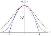
Figure 4: The early stage profile at $t=0.04$ calculated from the truncated parabolic initial condition (solid curve) is compared with the short-time self-similarity prediction (lower dashed curve) and with the late-stage one (upper dashed curve).

III.3 Short-Time Self-Similarity in Space and Time of Capillary-Driven Thin-Film Equation

The capillary evolution of the profile of the free surface of a thin viscous liquid film occurs as the quasi-static balance between the Laplace pressure and the viscous force due to the flow (see [11] and the references cited therein). The time evolution of the height profile function, $u(x,t),$ obeys the fourth-order partial differential equation:

$${\frac{\partial u}{\partial t}=-\frac{\partial^{4}u}{\partial x^{4}}.}$$ (8)

The system allows the self-similarity, ${u(x,t)=t^{-\frac{\beta+1}{4}}\,\phi({x}{t^{-{\frac{1}{4}}}}),}$ where the scaling function $\phi(s)$ with $s=xt^{-{\frac{1}{4}}},$ should obey

$${-\phi^{\prime\prime\prime\prime}(s)+\frac{s}{4}\phi^{\prime}(s)+\frac{\beta+1}{4}\phi(s)=0.}$$ (9)

Most generally the solution $\phi(s)$ or its derivative $\phi^{\prime}(s)$ do not decay rapidly for a given value of $\beta.$ Equation (9) under a given $\beta$ allows two independent even solutions of which one solution can have the power-low asymptote $\phi(s)\sim|s|^{-(\beta+1)}.$ In [11], the special case corresponding to $\beta=0$ with rapidly decaying derivative has been analyzed. As in the case of diffusion, the scaling function with power-law asymptote implies the static algebraic asymptote in space, $u(x,t)\sim|x|^{-(\beta+1)}$ ($|x|\gg t$), because  the algebraic asymptote of $\phi(s)$ issues from the balance of the last two terms on the left-hand side of Equation (9), which in turn implies $\partial u/\partial t\simeq 0$. Figure 5 shows, in the scaled coordinates, the evolution from the wedge-like initial configuration, which corresponds to $\beta=-2.$

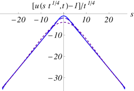
Figure 5: Short-time self-similarity evolution with algebraic asymptote of capillary-driven thin-film equation. From the initial profile $u(x,0)=1-|x|$ (this cannot be shown on this plane), the solution $u(x,t)$ for Equation (8) at $t=1$ (solid curve), $t=2^{4}$ (long dashed curve) and $t=2^{8}$ (short dashed curve) are presented using the scaled variables. The scaling function, which is numerically obtained by solving Equation (9) with $\beta=-2,$ is almost indistinguishable with the earliest profile (solid curve).

Unlike the simple diffusion, identifying the solution with algebraic asymptote requires a tuning of the ratio $\phi^{\prime\prime}(0)/\phi(0)$ (e.g., at $0.739\ldots$ for Figure 5) because the other solution of the same parity grows with $|s|$ faster than any power-laws. Zhang and Lister [12], in their study of the rupture of thin film by the van der Waals interaction, discussed how the inclusion of nonlinearity in the evolution equation selects the value of the exponent $\beta$ to some discrete ones.

IV Conclusions

The fact that solutions to many differential equations enjoy the property of self-similarity is well known for about hundred years (see, e.g., the book by L.I. Sedov [2]). In this paper, we show the existence of transformation that internally relates among the solution family of the scaling function (Figure 1). The concrete transformation consists of an integrating factor, which is the solution of adjoint equation and a Wick-rotation type transformation.

To the authors’ knowledge, this type of symmetry has not been reported before. How general is such structure for the evolution systems other than the diffusion remains a future problem. The existence of such transformation might not be specific for the differential equations of scaling functions. However, it is physically interesting and new that this transformation relates the self-similar relaxation process with flux-free boundary on the one hand (i.e., $\phi_{p}$ with $p\geq 0$) and the self-similar process with steady flux at boundary on the other hand ($\phi_{p}$ with $p\leq-1$).

We show the utility of the self-similarity in space and time to analyze the early stage of diffusive processes including the pure diffusion as well as the thin-film equation. These types of self-similarity focus on the local process in space-time and, therefore, are distinguished from the late-stage ones. The merit of the short-time similarity is that, even if the whole system has characteristic lengths or times, the self-similarity in the local space-time region works at the scale which is far below those characteristic scales . In Section III, we show the utility of the scaling functions that decay or grow algebraically. The short-time self-similarity of diffusion from smooth peak or wedge-like apex are new physical results, and so is the short-time self-similar solution of the surface diffusion. Unlike that of Benzaquen et al. [11], the latter solution has algebraic tails. Generically, one can prepare any algebraically decaying tail as initial condition for which the approach taken in Section III.2 will be useful, or at least usable. In the application of self-similar solution with algebraic tail to the relaxation of gel (Section III.1), we bring a new physical idea of combining the elastic aspect of gel, which is described by hyperbolic or elliptic equations, and the diffusive aspect, which obeys parabolic equations. By the former aspect, we can prepare an algebraic tail, and afterwards the gel shows self-similar relaxation having algebraic tail.

In some fields of research [2], the main idea of considering scaling relations is the use of these relations for constructing unknown solutions to the equations whose physical behavior is yet to be clarified. In the present paper, we do the opposite. We take simple equations with well or less known solutions and state that, for some specially constructed initial conditions, scaling with respect to space and time variables occurs. In the future, these two approaches might meet, where the internal relationship among the solution family will help to understand the global picture.

Lastly, the application might not be limited to the linear systems. One apparent example is the Burgers equation, since this equation can be reduced to the diffusion equation through the Cole–Hopf transformation if the boundary conditions are compatible [13]. Other type of generalization remains as an open question. When some mathematical objects represents well some physical phenomena, the mathematical relationship among the former might well have some physical consequences in the latter. We would like to know in the future the meaning of the transformation in Section II in physics terms.

Appendix A Family of Scaling Functions for the Self-Similarity Solution of 1D Diffusion Equation

When $q$ is non-negative integer, the adjoint equation $\mathcal{L}^{\dagger}_{q}\psi_{q}(s)=0$ has a polynomial solution, $\psi_{q}(s)=H_{q}({s}/{2})$ up to a multiplicative constant, where $H_{q}(x)$ is the $q$th-order Hermite polynomial function. By the symmetry presented in the main text, the polynomial solution of $\mathcal{L}_{p}\phi_{p}(s)=0$ with $p+q+1=0$ is $\phi_{p}(s)=H_{q}({is}/{2}).$ For non-integer or negative values of $q,$ the symmetric solution satisfying ${\phi}_{p}^{\rm(s)}(0)=1,$ and ${\phi}_{p}^{\rm(s)\prime}(0)=0$ is ${\phi}_{p}^{\rm(s)}(s)=e^{-\frac{s^{2}}{4}}{{}_{1}\!F_{1}}\left(-\frac{p}{2},{\frac{1}{2}},\frac{s^{2}}{4}\right)$ and the antisymmetric solution satisfying ${\phi}_{p}^{\rm(a)}(0)=0,$ and ${\phi}_{p}^{\rm(a)\prime}(0)=1$ is ${\phi}_{p}^{\rm(a)}(s)=s\,e^{-\frac{s^{2}}{4}}{{}_{1}\!F_{1}}\left(\frac{1-p}{2};\frac{3}{2};\frac{s^{2}}{4}\right),$ where ${{}_{1}\!F_{1}}(a;b;z)$ is the confluent hypergeometric function of the first kind [14, 15].

Table 1:

p	$\Phi_{p,e}(s)$	$\Phi_{p,o}(s)$
$-$3	$\Phi_{-3,e}(s)=\frac{s^{2}}{2}+1$	$\Phi_{-3,o}(s)=\frac{\sqrt{\pi}}{2}(\frac{s^{2}}{2}+1)\,{\rm erf}(\frac{s}{2})+\frac{s}{2}e^{-\frac{s^{2}}{4}}$
$-$2	${\Phi_{-2,e}(s)=\frac{\sqrt{\pi}}{2}s\,{\rm erf}(\frac{s}{2})+e^{-{s^{2}}/{4}}}$	$\Phi_{-2,o}(s)=s$
$-$1	$\Phi_{-1,e}(s)=1$	$\Phi_{-1,o}=\sqrt{\pi}{\rm erf}(\frac{s}{2})$
0	$\Phi_{0,e}(s)=e^{-{s^{2}}/{4}}$  (*)	$\Phi_{0,o}(s)=e^{-{s^{2}}/{4}}\int_{0}^{s}e^{{w^{2}}/{4}}dw$
1	$\Phi_{1,e}(s)\propto\Phi^{\prime}_{0,o}(s)$	$\Phi_{1,o}(s)\propto\Phi^{\prime}_{0,e}(s)$  (*)
2	$\Phi_{2,e}(s)\propto\Phi^{\prime\prime}_{0,e}(s)$  (*)	$\Phi_{2,o}(s)\propto\Phi^{\prime\prime}_{0,o}(s)$

Figure 6: Examples of the scaling functions satisfying Equation (2) with power-law asymptotes. $\phi_{0,o}(s)=e^{-{s^{2}}/{4}}\int_{0}^{s}e^{{w^{2}}/{4}}dw$ (solid curve), $\phi_{1,e}(s)=\phi_{0,o}^{\prime}(s)$ (coarse dashed curve), and $\phi_{2,o}(s)=\phi_{0,o}^{\prime\prime}(s)$ (fine dashed curve). For $|s|\gg 1$, these functions decays as $\sim|s|^{-(p+1)}$ with $p=0,1,$ and $2$, respectively.

Appendix B Spacetime Self-Similarity Solution of Equation (7)

Into Equation (7), we substitute the form of the radial displacement,

$$U^{\rm(r,t)}=U_{p}^{\rm(r)}(r,t)\equiv{\frac{1}{(Dt)^{\frac{p+1}{2}}}}\Psi_{p}{\left({\frac{r}{\sqrt{Dt}}}\right)}.$$

We then obtain the ordinary differential equation for $\Psi_{p}(s)$ with $s>0$:

$${2s^{2}\Psi_{p}^{\prime\prime}(s)+s(s^{2}+4)\Psi_{p}^{\prime}(s)+((p+1)s^{2}-4)\Psi_{p}(s)=0.}$$ (10)

In addition to the far field condition, $\Psi_{p}(\infty)=0,$ we impose the boundary condition at $s=0$, which is compatible with the homogeneous dilatation around the origin. In terms of the displacement vector field $\vec{U},$ the homogeneous dilatation reads $\vec{U}(\vec{r},t)=c(t)\,\vec{r}+{\cal O}(r^{3})$ for $r\downarrow 0$ with $c(t)$ being a function of time. We then impose $\Psi_{p}(0)=0.$ Under these boundary conditions, the solutions of Equation (10) is written in terms of the confluent hypergeometric function ${}_{1}\!F_{1}(a;b;z)$ [14, 15]. The solution reads

$${\Psi_{p}(s)=\Psi^{\prime}_{p}(0)\,s\times\,_{1}\!F_{1}{\left({1+\frac{p}{2};\frac{5}{2};-\frac{s^{2}}{2}}\right)}.}$$ (11)

This solution behaves as $\Psi_{p}(s)\simeq\Psi^{\prime}_{p}(0)\times s$ for $0\leq s\ll 1$ and $\Psi_{p}(s)\sim s^{-(p+1)}$ for $s\gg 1.$ Because $U_{\rm rad}(r,0)\sim r^{-2}$ for $r\gg t^{{\frac{1}{2}}},$ we choose $p=1,$ then we have

$${\Psi_{1}(s)=\Psi^{\prime}_{1}(0)\times\frac{6}{s^{2}}{\left[{-s\,e^{-\frac{s^{2}}{4}}+\sqrt{\pi}{\rm erf}{\left({\frac{s}{2}}\right)}}\right]}.}$$ (12)

References

References

- Barenblatt [1996] Barenblatt, G.I. Scaling, Self-Similarity, and Intermediate Asymptotics; Cambridge University Press: Cambridge, UK, 1996.
- Sedov [1959] Sedov, L. Similarity and Dimensional Methods in Mechanics; Academic Press: Cambridge, MA, USA, 1959.
- Hohenberg and Halperin [1977] Hohenberg, P.C.; Halperin, B.I. Theory of dynamic critical phenomena. Rev. Mod. Phys. 1977, 49, 435–479, doi:10.1103/RevModPhys.49.435.
- Gunton and Droz [1983] Gunton, J.; Droz, M. Introduction to the Theory of Metastable and Unstable States; Springer: Berlin/Heidelberg, Germany, 1983.
- Mansfield [1999] Mansfield, E.L. The Nonclassical Group Analysis of the Heat Equation. J. Math. Anal. Appl. 1999, 231, 526–542.
- Bluman and Cole [1969] Bluman, G.W.; Cole, J.D. The General Similarity Solution of the Heat Equation. J. Math. Mech. 1969, 18, 1025–1042.
- Tanaka et al. [1973] Tanaka, T.; Hocker, L.O.; Benedek, G.B. Spectrum of light scattered from a viscoelastic gel. J. Chem. Phys. 1973, 59, 5151–5159.
- de Gennes [1979] de Gennes, P.G. Scaling Concepts in Polymer Physics; Cornell University Press: Ithaca, NY, USA, 1979.
- Sekimoto and Fujita [2012] Sekimoto, K.; Fujita, T. Family of self-similar solutions of diffusion equation—Structure and Properties. arXiv 2012, arXiv:math.AP/1211.0935.
- Christov and Stone [2012] Christov, I.C.; Stone, H.A. Resolving a paradox of anomalous scalings in the diffusion of granular materials. Proc. Natl. Acad. Sci. USA 2012, 109, 16012–16017.
- Benzaquen et al. [2013] Benzaquen, M.; Salez, T.; Raphaël, E. Intermediate asymptotics of the capillary-driven thin-film equation. Eur. Phys. J. E 2013, 36, 82.
- Zhang and Lister [1999] Zhang, W.W.; Lister, J.R. Similarity solutions for van der Waals rupture of a thin film on a solid substrate. Phys. Fluids 1999, 11, 2454–2462.
- Hopf [1950] Hopf, E. The partial differential equation . Comm. Pure Appl. Math. 1950, 3, 201–230.
- [14] Weisstein, Eric W. “—Confluent Hypergeometric Function of the First Kind.” From MathWorld—A Wolfram Web Resource.
- Abramowitz and Stegun [1965] Abramowitz, M.; Stegun, I.A. Handbook of Mathematical Functions with Formulas, Graphs, and Mathematical Tables; National Bureau of Standards Applied Mathematics Series; Dover: London, UK, 1965; Volume 55, p. 503.