Theoretical investigation into the possibility of very large moments in Fe₁₆N₂

Abstract

We examine the mystery of the disputed high-magnetization $\alpha^{\prime\prime}$-Fe₁₆N₂ phase, employing the Heyd-Scuseria-Ernzerhof screened hybrid functional method, perturbative many-body corrections through the GW approximation, and onsite Coulomb correlations through the GGA+U method. We present a first-principles computation of the effective on-site Coulomb interaction (Hubbard $U$) between localized 3$d$ electrons employing the constrained random-phase approximation (cRPA), finding only somewhat stronger on-site correlations than in bcc Fe. We find that the hybrid functional method, the GW approximation, and the GGA+U method (using parameters computed from cRPA) yield an average spin moment of 2.9, 2.6 – 2.7, and 2.7 $\mu_{B}$ per Fe, respectively.

I Introduction

Though discovered in 1951 by Jack,jack $\alpha^{\prime\prime}$-Fe₁₆N₂ (with crystal structure pictured in Figure 1) first drew the attention of the magnetics community in 1972. It was then, 20 years later, that Kim and Takahashikt reported polycrystalline, mixed-phase Fe-N films with a saturation magnetization exceeding that of both $\alpha$-Fe and Co₃₅Fe₆₅ ($\sim 2\times 10^{6}$ A/m). However, it took another 20 years for the result to be reproduced (and, in fact, surpassed) by Sugita et al.sugita1 ; sugita2 Throughout the 1980s and ’90s, other measurements of Fe₁₆N₂ thin films were reported that generally did not find this large magnetic moment.kano ; nakajima ; mtaka1 ; mtaka2

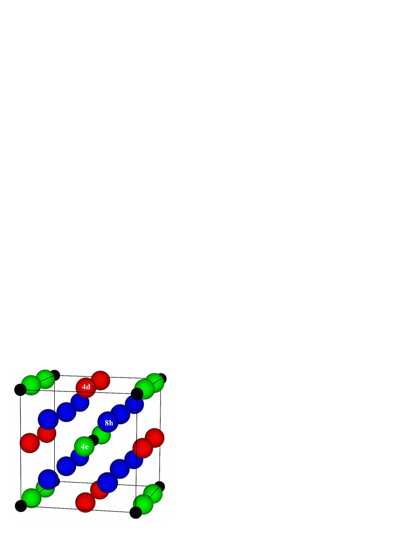
Figure 1: (color online) Crystal structure of Fe₁₆N₂, belonging to space group $I4/mmm$. We use the PBE-relaxed structure in all calculations with $a=5.72$ Å, $c=6.29$ Å, $x=0.243$, and $z=0.294$. We will frequently refer to the three inequivalent Fe Wyckoff sites: $4d$ (red), $4e$ (green), and $8h$ (blue) (the N sites are black).

Concurrently, density-functional theory (DFT) electronic structure calculations were performed,coehoorn ; coey ; sakuma ; ishida1 ; ishida2 ; min finding the moment per Fe ion to be modestly increased with respect to bulk bcc Fe but far short of the 3.5 $\mu_{B}$ reported by Sugita et al. It was shownlai that LSDA+Ulsdau calculations could yield an average moment comparable to that of some experiments ($\sim 2.8\mu_{B}$ per Fe), but the parameters ($U\approx 3.94$, 1.0, and 1.34 eV on the $4d$, $4e$, and $8h$ sites, respectively, with $J=U/10$) were obtained via an embedded-cluster method with a small screening constant and were not calculated from first principles. Additionally, the $J$ parameter is smaller than usually considered appropriate for transition metals (typically one chooses either an atomic-like $J$ of about $0.9$ eV or else a more screened $J$ of about 0.6-0.7 eV).

Recently, further experimental evidence for the large magnetization has arisen,ji_expt as well as a companion theoretical paperji_theor reporting enlarged Fe moments achieved using LSDA+U (using $U=1.0$ eV for the $4d$ site, 4.0 eV for the $4e$ and $8h$ sites, and $J$ = $U/10$). Ji et al. motivate their parameters by proposing that the Fe sites in the N-Fe octahedra form strongly correlated clusters in a metallic Fe environment, choosing a small $U$ for the (within their model) more metallic $4d$ sites and a large $U$ (chosen to be intermediate between that of FeO and Fe) for the $4e$ and $8h$ sites. They suggest that this model is supported by XMCD spectra that show additional features at the Fe sites not seen in bcc Fe or other Fe-N phases.wang

In the present work, we perform an extensive search for the proposed large magnetization; we calculate the hyperfine field at the three Fe sites and compare with published Mössbauer spectra; we search for additional energy minima at moments away from the theoretical prediction as a function of tetragonal distortion; we apply the HSE06 hybrid-functional methodhse06 and the GW approximationgw as implemented in VASPvasp to $\alpha^{\prime\prime}$-Fe₁₆N₂, testing the two methods on bcc Fe to ensure that any enhancement of the moment we obtain is genuine. Further, we compute the effective on-site Coulomb interaction (Hubbard $U$) between localized 3$d$ electrons employing the constrained random-phase approximation (cRPA) cRPA ; Sasioglu ; cRPA_Sasioglu (as implemented in the SPEXSpex extension of the FLEURFleur code), allowing us to provide for the first time first-principles predictions for the $U$ and $J$ parameters. Finally, we present new PBE+Upbe calculations using these parameters and discuss their implications for existing models.

II Computational Details

The hyperfine field calculation and the study of the dependence of the total energy on cell moment (fixed spin moment or FSM) and tetragonal distortion was performed using the FPLO code.Koepernik1999 We implemented the full relativistic expression for the hyperfine field

$$B_{HF} = \frac{\hbar^{2}}{ecm_{e}}\sum_{\nu}\left\langle\nu\left|\underline{\bm{\alpha}}\cdot\left(\hat{\bm{\mu}}_{n}\times\frac{\mathbf{r}}{r^{3}}\right)\right|\nu\right\rangle$$ (1)

as given in Ref. Severin1997, and references therein into FPLOKoepernik1999 . Note, that here we give the general pre-factor to accomodate for proper units. $|\nu\rangle$ are the solutions of the Kohn-Sham-Dirac equation, while $\underline{\bm{\alpha}}=\left(\begin{array}[]{cc}0&\bm{\sigma}\\ \bm{\sigma}&0\end{array}\right)$, with $\bm{\sigma}$ being the vector of the Pauli matrices. $\hat{\bm{\mu}}_{n}$ is the direction of the nuclear spin moment. The wave functions $\Psi_{\nu}$ are expanded in local atom centered orbitals in FPLO. The effective integrand $\frac{1}{r^{2}}$ leads to a damping factor for matrix elements between orbitals from different sites, which allows to introduce the approximation that only terms with orbitals belonging to the atom at which the nuclear spins sits will be taken into account. The scalar relativistic hyperfine fields only contains the Fermi contact term, while the full relativistic version contains all terms (including Fermi contact, orbital and spin dipole-nuclear dipole), due to the intrinsic 4-component formulation of Eq. (1) and the use of 4-spinors. A non-relativistic limit of this expression reveals all of the separate terms. The major contributions come form the $s$-orbitals, for whom only the Fermi contact term contributes. Although, the core states contribute a large amount to the hyperfine field it has been shownEbert1996 that valence contributions can be sizable. The core contribution depends on the spin polarization of the core wave functions including the effects of the crystal exchange potential and hence should be influenced and scaled by the local spin moment. In FPLO the semi-core (Fe 3s,3p) states are treated like valence states. For this reason we include the valence and semi-core contributions via the onsite approximation as explained above.

The FSM calculation was carried out within the PBE approximation using a $8\times 8\times 8$ $k$-point mesh in a linear tetrahedron method with Blöchl corrections. Our VASP PBE+U (using the fully-local double-counting term), HSE06 and GW calculations used a plane-wave cut-off of 400 eV (29.4 Ry or 5.42 $a_{0}^{-1}$). The PBE+U (HSE06 and GW) calculations used an $8\times 8\times 8$ ($6\times 6\times 6$) $\Gamma$-centered Monkhorst-Pack $k$ mesh (also using the tetrahedron method with Blöchl corrections), employing a smaller $3\times 3\times 3$ mesh for the exact-exchange sums. All of our VASP calculations use the PAWpaw pseudopotentials of Kresse and Joubert,kressepp and all VASP moments are calculated within a sphere of radius 1.3 Å on the Fe sites.

To calculate the Hubbard $U$ parameter we employ the constrained random-phase approximation (cRPA) cRPA within the full-potential linearized augmented-plane-wave (FLAPW) method using maximally localized Wannier functions (MLWFs). cRPA_Sasioglu ; Max_Wan The cRPA approach offers an efficient way to calculate the effective Coulomb interaction $U$ and allows to determine individual Coulomb matrix elements, e.g., on-site, off-site, inter-orbital, intra-orbital, and exchange as well as their frequency dependence. We use the FLAPW method as implemented in the FLEUR code Fleur with the PBE exchange-correlation potentialpbe for ground-state calculations. A dense $16\times 16\times 16$ $\mathbf{k}$-point grid is used. The MLWFs are constructed with the Wannier90 code Wannier90 ; Fleur_Wannier90 . The effective Coulomb potential is calculated within the recently developed cRPA method cRPA implemented in the SPEX code Spex (for further technical details see Refs. Sasioglu, , cRPA_Sasioglu, , and mpb, ). We use a $3\times 3\times 3$ $k$-point grid in the cRPA calculations.

In all calculations we use the PBE-relaxed structure with $a=5.72$ Å and $c=6.29$ Å (except in the FSM survey) and internal parameters $x=0.243$ and $z=0.294$. As a final note, we consider all employed electronic structure schemes (VASP, FLEUR, FPLO) to be equivalent with respect to numerical accuracy at the level required in the present study. The use of three different packages is motivated by the different implementations available in these codes.

III Results and Discussion

III.1 Hyperfine Field

The hyperfine field provides a picture of the local magnetic structure that, unlike measurements of the saturation magnetization, does not require accurate estimation of the volume of a sample or its component phases. Mössbauer spectroscopy has been performed in many previous worksmoriya ; sugita1 ; sugita2 ; mtaka2 ; ortiz ; nakajima2 ; okamoto , and the hyperfine field has been calculatedcoehoorn ; ishida1 ; ishida2 ; coey2 from DFT. Our calculated $B_{hf}$ (found along with our calculated Fe moments in Table 1) agrees well with these past results; we find that the Fe sites with N nearest-neighbors exhibit approximately the same field (-23 and -22 T on the $4e$ and $8h$ sites), while $B_{hf}=-31$ T for the $4d$ sites. If we note, as previous authors have,coehoorn that DFT underestimates the hyperfine field by a substantial, though nearly static, amount ($\sim 8$ T in this case), then we also find reasonable agreement with some of the experimental reports. Particularly, we agree well with Refs. mtaka2, , moriya, , and ortiz, . Although our hyperfine fields agree numerically with those of Moriya et al.,moriya they claimed that the largest hyperfine field was to be found in the $8h$ site, a claim that is difficult to reconcile with the predicted relative magnitudes of the moments and the similar environment of the $4e$ and $8h$ sites. We note, however, that this assignment of the hyperfine fields agrees better with the moments in the recent LSDA+U study of Ji et al..ji_theor We cannot offer any new explanation for Sugita et al.’s larger 46 T fieldsugita1 nor the presence of only one Mössbauer sextet in their later single-phase sample.sugita2

Site	Spin Moment ($\mu_{B}$)	$B_{hf}$ (T) (scal.-rel.)	$B_{hf}$ (T) (rel.)
$4d$	2.85	-34	-31
$4e$	2.17	-25	-23
$8h$	2.36	-25	-22

Table 1: Spin moments calculated within scalar-relativistic PBE and hyperfine fields (both fully- and scalar-relativistic) for each Fe site calculated within PBE using the FPLO code.

III.2 Fixed Spin-Moment Survey

Generally, expansion of the lattice may not be an efficient means of increasing the magnetization of a material, as the enhancement of the spin moments may not outpace the increase in volume. However, it is known that fcc Fe, while ordinarily nonmagnetic, enters a high spin state upon expansion of the cell volume.fccFe Therefore, we have explored the energy landscape as a function of total (spin) cell moment and $\frac{c}{a}$, allowing the former to range from 34 – 48 $\mu_{B}$ (corresponding to average spin moments of 2.12 – 3.0 $\mu_{B}$ per Fe) and the latter from 1.0 – 1.5 (holding $a$ fixed in one set of calculations and volume fixed in another). We only constrain the total spin moment of the cell and not the magnitude of the individual moments. In principle, the moments of the three inequivalent Fe sites could be arranged in many ways to obtain the same total spin moment; however, we simply accept the converged result for each structure and total moment without seeking out other possible minima.

The results may be seen in Figure 2. We note that no additional local energy minima were observed apart from the PBE-relaxed structure ($a=5.72$ Å, $c=6.29$ Å, $c/a\approx 1.10$) and moment (2.44 $\mu_{B}$). Although the energy minimum does tend to shift to higher moments with the increase of the volume through $\frac{c}{a}$, the enhancement is not sufficient to produce an increase in the magnetization. With $a$ held fixed at $a_{\text{expt}}=5.72$ Å, the average spin moment per Fe reaches 2.81 $\mu_{B}$ at $\frac{c}{a}=1.5$, giving a magnetization of $1.49\times 10^{6}$ A/m, compared to $1.77\times 10^{6}$ A/m at the experimental $\frac{c}{a}$ and $1.75\times 10^{6}$ A/m in bcc Fe. If the volume is held fixed, the average moment does not depend strongly on $\frac{c}{a}$, remaining close to the PBE value throughout and decreasing to about $2.25\mu_{B}$ at $\frac{c}{a}=1.5$. This supports the standard understanding of the LSDA- or GGA-predicted increase in the moment as arising from increased cell volume.

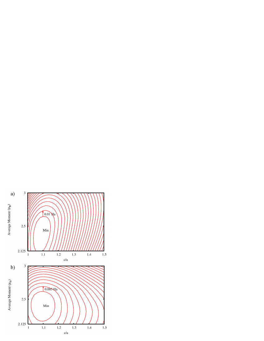
Figure 2: (color online) Energy landscape of Fe₁₆N₂ as a function of tetragonal distortion and average moment per Fe with a) $a$ held fixed and b) volume held fixed. Each contour represents an increase of a) 10 mHa (0.27 eV) or b) 5 mHa (0.14 eV). There are no additional local energy minima in the parameter space examined. For fixed $a$, $\frac{c}{a}=1.5$ gives $\mu_{avg}=2.81\mu_{B}$. Although the average moment is higher at this point, it does not overcome the increase in volume, and the magnetization is only 84% of the magnetization of the PBE structure. For fixed volume, the average moment remains close to the PBE value, decreasing slightly as $c$ increases above $\sim 1.1a$.

III.3 HSE06 and GW

It is possible that DFT cannot fully account for the physics that would give rise to greatly enhanced magnetization in $\alpha^{\prime\prime}$-Fe₁₆N₂, so we have also considered methods that have arisen since the last wave of theoretical investigation into this material subsided. The HSE06 screened hybrid functional method entails only a moderate increase in computational time with respect to PBE, and the inclusion of a static screening parameter for the exact exchange term allows for the treatment of metallic systems—unlike the parent Hartree-Fock method—as well as speeding up calculation further. HSE06 follows PBE0 in its formulation of the exchange-correlation energy, given by

$$E_{xc}=\frac{1}{4}E_{x}^{HF,SR}+\frac{3}{4}E_{x}^{PBE,SR}+E_{x}^{PBE,LR}+E_{c}^{PBE}$$ (2)

The aforementioned screening parameter $\mu=0.2$ Å^-1 partitions the exchange term into a short-range and a long-range component, achieved by appending erfc$(\mu r)$ (the complementary error function) to the short-range terms and erf$(\mu r)$ to the long-range term.hse06

The GW approximation improves upon Hartree-Fock by treating electrons as dressed quasiparticles interacting via a screened Coulomb operator $W$. This replaces the purely real exchange-correlation potential with a complex self energy $\Sigma=-iGW$. In the initial step, the Green’s function $G$ and the screened Coulomb operator $W$ are calculated from the wave functions obtained from a converged DFT calculation. The computation of $W$ via the RPA is time-consuming, and consequently some shortcuts are sometimes employed. So-called “one-shot” GW or G₀W₀ is performed by calculating the quasiparticle energies using only these initial quantities and yields improved results compared to LSDA.faleev ; vsg Nevertheless, the “one-shot” method still underestimates band-gaps due to the inaccuracies inherent in using an LSDA-obtained $W$, and improvement can be obtained by iterating $G$ and $W$ to self-consistency. We present results from G₀W₀, GW₀, and GW in this work.

Figure 3 shows the partial density of states (pDOS) of each Fe site in HSE06 and GW. For comparison, we include the PBE-calculated pDOS for Fe₁₆N₂ and a fictitious “Fe₁₆N₀” structure obtained by removing the N atoms without relaxing the structure. This latter case shows that, within PBE, Fe approaches the strong ferromagnetic state, with the majority $d$ states nearly fully occupied, upon the N-induced volume expansion, yielding an average moment of 2.56 $\mu_{B}$ per Fe and a magnetization of $1.84\times 10^{6}$ A/m, about a 5% increase over bcc Fe (with a bulk magnetization of $1.75\times 10^{6}$ A/m). The HSE06 pDOS shows a greatly enhanced exchange splitting with respect to PBE-Fe₁₆N₀ and GW-Fe₁₆N₂, leading to an average moment of 2.86 $\mu_{B}$ per Fe ($M=2.06\times 10^{6}$ A/m), whereas GW yields a more moderate 2.57-2.70 $\mu_{B}$ per Fe ($M=1.85$–$1.95\times 10^{6}$ A/m). The calculated spin moment at each site can be found in Table 2.

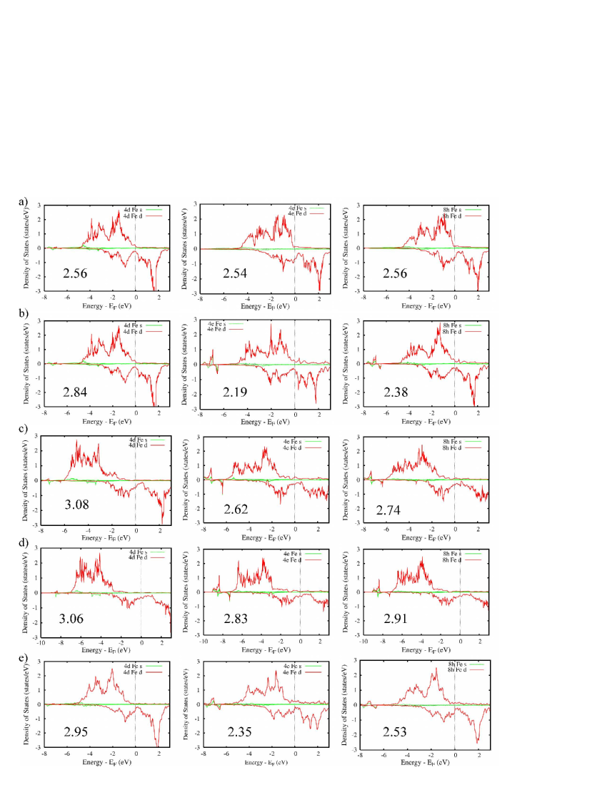
Figure 3: (color online) $s$ and $d$ Partial density of states and spin moments (in $\mu_{B}$) for the $4d$, $4e$, and $8h$ Fe sites (left, middle and right columns) for a) a fictitious Fe₁₆N₀ structure (within PBE) in which the Fe atoms retain their $\alpha^{\prime\prime}$ positions. Here, we see that the majority channel is already nearly fully occupied due to the volume expansion induced by the N atoms. (b) PBE pDOS showing the effect of Fe – N hybridization: increasing the moment of the second-neighbor $4d$ site at the expense of the $4e$ and $8h$ sites. (c-e) PBE+U, HSE06, and GW₀, respectively (the reader should note the difference in the scale of the $x$ axis in the HSE plots): PBE+U and HSE06 each give large moments at each site, but predict an average moment only slightly larger than in bcc Fe (for which they also give very large moments). The pDOS for all VASP-GW methods considered in the text are in qualitative agreement with those displayed.

Method	$4d$ Site ($\mu_{B}$)	$4e$ Site ($\mu_{B}$)	$8h$ Site ($\mu_{B}$)	Average ($\mu_{B}$)	bcc Fe ($\mu_{B}$)
PBE	2.84	2.19	2.38	2.44	2.23
PBE+U	3.08	2.62	2.74	2.71	2.67
HSE06	3.06	2.83	2.91	2.86	2.85
G0W0	2.90	2.31	2.49	2.57	2.33
GW0	2.95	2.35	2.53	2.64	2.62
GW	2.96	2.41	2.57	2.66	2.65
GW ($s,p$ val.)	3.00	2.50	2.64	2.70	2.59

Table 2: Calculated spin moments for all methods presented in this work. The PBE+U results were obtained using the cRPA-obtained interaction parameters $U=3.99$, 3.12, and 3.52 eV for the $4d$, $4e$, and $8h$ sites, respectively ($J=0.64$, 0.59, and 0.61 eV), except for bcc Fe, for which we used $U=3.16$ eV and $J=0.68$ eV as in Ref. cRPA_Sasioglu, . GW ($s,p$ val) denotes a VASP-GW calculation in which the Fe $3s$ and $3p$ electrons are treated on the same level as the $3d$ and $4s$.

In the absence of experimental photo- or x-ray-emission data to which to compare, we must test the validity of the calculated moments by calculating the moments of better established materials. The last column in this table shows the calculated spin moment for bcc Fe from PBE, PBE+U (which will be discussed in detail in the following section), HSE06, and GW. Our HSE06 result for bcc Fe agrees with previous workjang and demonstrates that, although the screened hybrid functional method improves on the Hartree-Fock treatment of metallic systems, it can overestimate the strength of the exchange and yield un-physical high spin states. However, we also note that the calculated bcc Fe spin moment is not necessarily directly proportional to the calculated moments in $\alpha^{\prime\prime}$-Fe₁₆N₂, so it is possible that the bcc Fe moment does not completely determine the accuracy of a method in this case.

III.4 cRPA and PBE+U

Previous attempts to explain the experiments that find high-magnetization have turned to LDA+U to describe the correlation effects that may be present in $\alpha^{\prime\prime}$-Fe₁₆N₂. However, as no first-principles calculations of the interaction parameters existed, it was necessary to motivate the choice of $U$ (and $J$) by analogy with other systems or by applying a model. In particular, the explanation for the enhanced magnetization proposed by Ji et al.ji_expt ; ji_theor and Wang et al.wang requires that the Fe sites with N nearest-neighbors be more strongly-correlated than the $4d$ sites, which have no N neighbors. Without a set of firmly-established parameters, it is difficult to progress in understanding this system, as the calculated moment is directly dependent on $U$ and $J$ (see, e.g. Figure 3 in Ref. ji_theor, ).

Recently, the cRPA has been proposed as a first-principles method of obtaining the screened Coulomb matrix within a Wannier basis.cRPA ; Sasioglu ; cRPA_Sasioglu Within the RPA, the polarizability $P$ can be written

$$P(\mathbf{r},\mathbf{r}^{\prime},\omega)=\sum_{\sigma}\sum_{n}^{\text{occ}}\sum_{m}^{\text{unocc}}\left[\frac{\psi^{*}_{\sigma{}n}(\mathbf{r})\psi_{\sigma{}m}(\mathbf{r})\psi^{*}_{\sigma{}m}(\mathbf{r}^{\prime})\psi_{\sigma{}n}(\mathbf{r}^{\prime})}{\omega-\varepsilon_{\sigma{}m}+\varepsilon_{\sigma{}n}+i\delta}\right.$$

$$\left.-\frac{\psi_{\sigma{}n}(\mathbf{r})\psi^{*}_{\sigma{}m}(\mathbf{r})\psi_{\sigma{}m}(\mathbf{r}^{\prime})\psi^{*}_{\sigma{}n}(\mathbf{r}^{\prime})}{\omega+\varepsilon_{\sigma{}m}-\varepsilon_{\sigma{}n}-i\delta}\right],$$ (3)

where the $\psi_{i}$ and $\varepsilon_{i}$ are the DFT wave functions and their eigenvalues, and $\sigma$ runs over both spin channels. If one separates $P$ into $P_{d}$, containing the correlated orbitals, and $P_{r}$, containing the rest, and if one considers the unscreened Coulomb operator $v$, one can writecRPA ; cRPA_Sasioglu

$$U=[1-vP_{r}]^{-1}v$$ (4)

$$\tilde{U}=[1-UP_{d}]^{-1}U$$ (5)

The matrix elements of the effective Coulomb potential $U$ in the MLWF basis are given by

$$U_{\mathbf{R}n_{1}n_{3};n_{4}n_{2}}(\omega)=\iint w_{n_{1}\mathbf{R}}^{*}(\mathbf{r})w_{n_{3}\mathbf{R}}(\mathbf{r})U(\mathbf{r},\mathbf{r}^{\prime};\omega)$$

$$\times w_{n_{4}\mathbf{R}}^{*}(\mathbf{r}^{\prime})w_{n_{2}\mathbf{R}}(\mathbf{r}^{\prime})\>d^{3}r\>d^{3}r^{\prime},$$ (6)

where $w_{n\mathbf{R}}(\mathbf{r})$ is the MLWF at site $\mathbf{R}$ with orbital index $n$ and $U(\mathbf{r},\mathbf{r}^{\prime};\omega)$ is calculated within the cRPA. Strictly speaking, the Wannier functions are spin dependent. However, we find that this spin dependence affects the values only little. For simplicity, we ignore the spin dependence here and give the spin-averaged values in the following.

In our Spex-cRPA calculation, we choose the Fe $d$ orbitals as our correlated subspace and compute the interaction parameters found in Table 3. Quantities with tildes are obtained from the fully screened Coulomb matrix $\tilde{U}$, while plain symbols are the $sp$-screened quantities that enter into the PBE+U calculations. The $U$, $U^{\prime}$, and $J$ (and their fully-screened counterparts) are averaged at each site as follows:

$$U_{DFT+U}=F^{0}=\frac{1}{25}\sum_{m,n}U_{mnmn}$$ (7a)

$$U=\frac{1}{5}\sum_{m}U_{mmmm}$$ (7b)

$$U^{\prime}=\frac{1}{10}\sum_{m<n}U_{mnmn}$$ (7c)

$$J=\frac{1}{10}\sum_{m<n}U_{mnnm}$$ (7d)

Site	$U_{DFT+U}$	$U$	$U^{\prime}$	$J$	$\tilde{U}$	$\tilde{U}^{\prime}$	$\tilde{J}$
$4d$	3.99	5.02	3.74	0.64	1.80	0.71	0.53
$4e$	3.12	4.14	2.95	0.59	1.56	0.55	0.49
$8h$	3.52	4.50	3.27	0.61	1.68	0.62	0.51

Table 3: The calculated on-site interaction parameters (all in eV) from cRPA for $\alpha^{\prime\prime}$-Fe₁₆N₂, showing a small increase in correlation with respect to bcc Fe. Quantities with a tilde are computed from the fully-screened Coulomb potential, while plain quantities are computed from the partially screened potential (omitting $d-d$ screening). $U_{DFT+U}$ is the $U$ parameter that enters into the PBE+U calculations.

We note that these parameters differ both quantitatively and qualitatively from previously proposed models, particularly those that suggest large differences in correlation strength between Fe sites. The spin moments from PBE+U, for Fe₁₆N₂ as well as bcc Fe, can be found in Table 2. The PBE+U spin moment for bcc Fe was calculated using the interaction parameters computed in Ref. cRPA_Sasioglu, —$U=3.16$ eV and $J=0.68$ eV. We use the fully-local (FLL) double counting correction in the calculation of both the bcc Fe and the Fe₁₆N₂ moments. Although this choice may seem strange in metallic systems, the around-mean-field (AMF) term opposes the formation of moments in generalYlvisaker2009 and here produces moments $\sim 1\mu_{B}$ below the expected value in bcc Fe. It should be noted, however, that the choice of the double counting term in PBE + U is not unique and thus leaves an ambiguity in the calculated moments even if $U$ and $J$ were computed with a well-defined method..

III.5 Orbital Moment

In solids, the orbital moment is typically nearly quenched, but in some extreme cases, such as UN,brooks the orbital moment can be comparable to the spin moment. PBE calculations give an orbital moment per Fe of only 0.05 $\mu_{B}$ in bcc Fe (Table 4), but this may be increased somewhat in Fe₁₆N₂. To explore this possibility, we calculated the orbital moment within PBE, PBE+orbital polarization correction (OPC),nordstrom PBE+U (using the cRPA parameters), and “one-shot” G₀W₀ using FPLO (for the OPC calculation) and VASP (for the rest). Each method shows a small increase in orbital moment compared to bcc Fe, yielding about 0.1 – 0.2 $\mu_{B}$ per Fe atom and an increase of 0.01 – 0.05 $\mu_{B}$ over bcc Fe. This small increase cannot explain those results that claim average Fe moments in excess of 3 $\mu_{B}$. Our PBE+U and G₀W₀ results predict average total (spin + orbital) moments of 2.88 and 2.63 $\mu_{B}$, respectively.

Method	$4d$ Site ($\mu_{B}$)	$4e$ Site ($\mu_{B}$)	$8h$ Site ($\mu_{B}$)	Average ($\mu_{B}$)	bcc Fe ($\mu_{B}$)
PBE	0.06	0.06	0.05	0.06	0.05
PBE+U	0.20	0.16	0.16	0.17	0.12
PBE+OPC	0.09	0.11	0.10	0.10	0.09
G0W0	0.06	0.06	0.05	0.06	0.05

Table 4: Calculated orbital moments in Fe₁₆N₂ within PBE, PBE+U, PBE+OPC, and G₀W₀. The orbital moment is increased by only 0.01 - 0.03 $\mu_{B}$ per Fe with respect to bcc Fe.

IV Summary

We have examined the electronic and magnetic structure of $\alpha^{\prime\prime}$-Fe₁₆N₂ within PBE, PBE+U, HSE06, and GW. Within PBE, we find spin moments and hyperfine fields that agree with past results, and we do not find that any high-magnetization state arises as $\frac{c}{a}$ changes from the experimental value. We have provided effective Coulomb interaction parameters calculated via cRPA and have used them in our PBE+U calculations. We find that PBE+U and HSE06 gives average spin moments per Fe of 2.71 and 2.86 $\mu_{B}$ but also greatly overestimate the moment of bcc Fe (experimentally about 2.2 $\mu_{B}$). GW gives smaller moments, 2.57 - 2.70 $\mu_{B}$ per Fe, a slight increase over the PBE moment. G₀W₀, GW₀, and GW all overestimate the bcc Fe spin moment by different amounts despite their similar predictions for Fe₁₆N₂, with G₀W₀ giving the most reasonable bcc Fe moment due to its close dependence on the PBE result. In all cases, we find that the $4e$ and $8h$ sites have smaller moments than that on the $4d$ site.

We have also presented calculations of the orbital moment on the Fe sites obtained within PBE, PBE+OPC, PBE+U, and G₀W₀. We find that the orbital moment is not completely quenched and may add 0.1 – 0.2 $\mu_{B}$ to the average total moment per Fe, a small increase over bcc Fe.

In order to evaluate the varying results found above, one must understand the purposes of and approximations inherent in the methods presented. In addition to the shortcomings of the mean-field-like treatment of correlations within PBE+U, there are two notable avenues for error in this method: the need to choose the $U$ and $J$ parameters and the lack of a priori justification for the double-counting corrections. Dependence on the choice of interaction parameters is not a fundamental problem and can be alleviated as we have done here by computing them through some appropriate first-principles method. The choice between the FLL or AMF double-counting corrections, while straightforward when treating insulators, can be less obvious in semi-localized magnetic systems, and furthermore no method exists for determining the exact form of the correction. The hybrid functional method’s dependence on parameters is fundamental to the approach, although it is mitigated somewhat by the use of predetermined parameters such as in HSE06. However, these parameters were primarily chosen to produce reasonable band gaps and may need to be altered to properly treat metallic systems. In principle, the GW approximation should be the most accurate of those presented here. The G₀W₀ and GW₀ methods maintain good contact with the PBE results while incorporating first-order exchange and correlation effects. However, some care must still be taken; we have shown that the results do depend on which electrons are treated as valence and which are absorbed into the core pseudopotential. Lastly, we note the need for additional, repeatable experiments that probe the electronic structure of the material in order to provide a better basis for comparison with theory.

V Acknowledgments

H.S. and W.H.B. acknowledge the support of NSF MRSEC Grant No. DMR-0213985 and the use of computing resources from the Alabama Supercomputer Center. M.R. would like to thank Joachim Wecker and Manfred Rührig for discussion. E.Ş, C.F and S.B. acknowledge the support of DFG through the Research Unit FOR-1346.

References

- (1) K. H. Jack, Proc. R. Soc. A 208, 200 (1951).
- (2) T. K. Kim and M. Takahashi, Appl. Phys. Lett. 20, 492 (1972).
- (3) Y. Sugita, K. Mitsuoka, M. Komuro, H. Hoshiya, Y. Kozono, and M. Hanazono, J. Appl. Phys. 70, 5977 (1991).
- (4) Y. Sugita, H. Takahashi, M. Komuro, K. Mitsuoka, and A. Sakuma, J. Appl. Phys. 76, 6637 (1994).
- (5) A. Kano, N. S. Kazama, H. Fujimori, and T. Takahashi, J. Appl. Phys. 53, 8332 (1982).
- (6) K. Nakajima and S. Okamoto, Appl. Phys. Lett. 56, 92 (1990).
- (7) M. Takahashi, H. Shoji, H. Takahashi, T. Wakiyama, M. Kinoshita, and W. Ohta, IEEE Trans. Magn. 29, 3040 (1993).
- (8) M. Takahashi, H. Takahashi, H. Nashi, H. Shoji, T. Wakiyama, and M. Kuwabara, J. Appl. Phys. 79, 5564 (1996).
- (9) R. Coehoorn, G. H. O. Daalderop, and H. J. F. Jansen, Phys. Rev. B 48, 3830 (1993).
- (10) J. M. D. Coey, J. Appl. Phys. 76, 6632 (1994).
- (11) A. Sakuma, J. Magn. Magn. Mater. 102, 127 (1991); A. Sakuma, J. Phys. Soc. Jpn. 60, 2007 (1991); A. Sakuma, J. Phys. Soc. Jpn. 61, 223 (1992).
- (12) S. Ishida and K. Kitawatase, J. Mag. Magn. Mat. 104-107, 1933 (1992).
- (13) S. Ishida, K. Kitawatase, S. Fujii, and S. Asano, J. Phys. Condens. Matter 4, 765 (1992).
- (14) B. I. Min, Phys. Rev. B 46, 8232 (1992).
- (15) W. Y. Lai, Q. Q. Zheng, and W. Y. Hu, J. Phys. Cond. Mat. 6, L259 (1994).
- (16) N. Ji, L. F. Allard, E. Lara-Curzio, and J.-P. Wang, Appl. Phys. Lett. 98, 092506 (2011).
- (17) N. Ji, X. Liu, and J.-P. Wang, New Journal of Physics 12, 063032 (2010).
- (18) V .I. Anisimov, J. Zaanen , and O.K. Andersen Phys. Rev. B 44, 943 (1991).
- (19) J.-P. Wang, N. Ji, X. Liu, Y. Xu, C. Sánchez-Hanke, Y. Wu, F. M. F. de Groot, L. F. Allard, and E. Lara-Curzio, IEEE Trans. Magn. 48, 1710 (2012).
- (20) J. Heyd, G. E. Scuseria, and M. Ernzerhof, J. Chem. Phys. 124, 219906 (2006).
- (21) L. Hedin, Phys. Rev. 139, A796 (1965).
- (22) G. Kresse and J. Furthmüller, Comput. Mater. Sci. 6, 15 (1996).
- (23) F. Aryasetiawan, M. Imada, A. Georges, G. Kotliar, S. Biermann, and A. I. Lichtenstein, Phys. Rev. B 70, 195104 (2004); F. Aryasetiawan, K. Karlsson, O. Jepsen, and U. Schönberger, Phys. Rev. B 74, 125106 (2006); T. Miyake, F. Aryasetiawan, and M. Imada Phys. Rev. B 80, 155134 (2009); B-C. Shih, Y. Zhang, W. Zhang, and P. Zhang, Phys. Rev. B 85, 045132 (2012); T. O. Wehling, E. Şaşıoğlu, C. Friedrich, A. I. Lichtenstein, M. I. Katsnelson, and S. Blügel, Phys. Rev. Lett. 106, 236805 (2011).
- (24) E. Şaşıoğlu, A. Schindlmayr, C. Friedrich, F. Freimuth and S. Blügel, Phys. Rev. B. 81, 054434 (2010).
- (25) E. Şaşıoğlu, C. Friedrich, and S. Blügel, Phys. Rev. B 83, 121101(R) (2011).
- (26) C. Friedrich, S. Blügel and A. Schindlmayr, Phys. Rev. B. 81, 125102 (2010).
- (27) http://www.flapw.de
- (28) J. P. Perdew, K. Burke, and M. Ernzerhof, Phys. Rev. Lett. 77, 3865 (1996).
- (29) L. Severin and M. Richter and L. Steinbeck, Phys. Rev. B 55, 9211 (1997).
- (30) K. Koepernik and H. Eschrig, Phys. Rev. B 59, 1743 (1999), http://www.fplo.de.
- (31) M. Battocletti and H. Ebert and H. Akai, Phys. Rev. B 53, 9776 (1996).
- (32) P. E. Blöchl, Phys. Rev. B 50, 17953 (1994).
- (33) G. Kresse and D. Joubert, Phys. Rev. B 59, 1758 (1999).
- (34) N. Marzari and D. Vanderbilt, Phys. Rev. B 56, 12847 (1997).
- (35) F. Freimuth, Y. Mokrousov, D. Wortmann, S. Heinze, and S. Blügel, Phys. Rev. B 78, 035120 (2008).
- (36) A. A. Mostofi, J. R. Yates, Y.-S. Lee, I. Souza, D. Vanderbilt, and N. Marzari, Comput. Phys. Commun. 178, 685 (2008).
- (37) C. Friedrich, A. Schindlmayr, and S. Blügel, Comp. Phys. Comm. 180, 347 (2009).
- (38) T. Moriya, Y. Sumitomo, H. Ino, and F. E. Fujita, J. Phys. Soc. Jpn. 35, 1378 (1973).
- (39) C. Ortiz, G. Dumpich, A. H. Morrish, Appl. Phys. Lett. 65, 2737 (1994).
- (40) S. Okamoto, O. Kitakami, Y. Shimada, J. Mag. Magn. Mat. 208, 102 2000.
- (41) K. Nakajima, T. Yamashita, M. Takata, and S. Okamoto, J. Appl. Phys. 70, 6033 (1991).
- (42) J M D. Coey, K. O’Donnell, Q. Qi, E. Touchais, and J. H. Jack, J. Phys. Cond. Mat. 6, L23 (1994).
- (43) V. L. Moruzzi, P. M. Marcus, K. Schwarz, and P. Mohn, Phys. Rev. B 34, 1784 (1986).
- (44) M. van Schilfgaarde, T. Kotani, and S. Faleev, Phys. Rev. Lett. 96, 226402 (2006).
- (45) S. V. Faleev, M. van Schilfgaarde, and T. Kotani, Phys. Rev. Lett. 93, 126406 (2004).
- (46) Y.-R. Jang and B. D. Yu, J. Mag. 16, 201 (2011).
- (47) M. S. S. Brooks and P. J. Kelly, Phys. Rev. Lett. 51, 1708 (1983).
- (48) E. R. Ylvisaker, W. E. Pickett, and K. Koepernik, Phys. Rev. B 79, 035103 (2009).
- (49) L. Nordström, M. S. S. Brooks, and B. Johansson, J. Phys.: Cond. Matt. 4, 3261 (1992).