KCL-PH-TH/2012-41

Using a non-perturbative approximation for the partition function of a complex scalar model, which features spontaneous symmetry breaking, we explicitly derive the flattening of the effective potential in the region limited by the minima of the bare potential. This flattening occurs in the limit of infinite volume, and is a consequence of the summation over the continuous set of saddle points which dominate the partition function. We also prove the convexity of the effective potential and generalize the Maxwell Construction for scalar theories with $O(N)$ symmetry. Finally, we discuss why the flattening of the effective potential cannot occur in the Abelian Higgs theory.

1 Introduction

The convexity of the effective potential for a scalar theory has been known for a long time [1], and is a consequence of its definition in terms of a Legendre transform [2]. In the situation where the bare potential features spontaneous symmetry breaking (SSB), convexity is achieved non-perturbatively, and cannot be obtained by a naive loop expansion. The effective potential becomes flat between the two minima of the bare potential, as a consequence of the competition of the two non-trivial saddle points [3]. By analogy with the Maxwell construction for a Van de Waals fluid, the corresponding flattening can be understood from the so-called spinodal instability: no restoration force suppresses fluctuations of the vacuum for the quantized system, which is a superposition of the two bare vacua [4]. A PhD thesis has been written on the topic [5], where many aspects are studied, and a detailed literature review is given.

We note that the equivalence between the effective potential defined via the Legendre transform and the Wilsonian effective potential is valid in the limit of infinite volume only [6], as the Wilsonian effective potential is not necessarily convex at finite volume. Lattice simulations of scalar SSB models in [6] show the gradual flattening for the Wilsonian effective potential (the “constrained effective potential”) as the number of lattice sites increases. On the other hand, as shown in the present work, the effective potential obtained by the Legendre transform is convex for finite volume too.

A linear effective potential was explicitly derived in [7], for a real scalar field in a SSB bare potential. Using a simple approximation, it was shown that the Maxwell construction arises from the dominant contributions of both saddle points in the partition function. These dominant contribution are homogeneous and do not take into account the kink solution, which is stable in 1+1 dimensions only if no other field is present [8]. We consider here two space dimensions at least (a recent work on the quantization of the 1+1 dimensional kink can be found in [9]).

Quantum corrections to the (Legendre) effective potential are calculable in series of $\hbar$ via functional techniques [10] as fixed-loop diagrammatic series. One- and two-loop corrections, computed in [10] for the $O(N)$ theory, do not suffice to restore convexity for a tree-level symmetry breaking potential. A large-N analysis, performed at the leading $1/N$ order in [11], leads to a real, convex potential in four dimensions albeit for a restricted range of field amplitudes, raising thus questions to the consistency of the scheme in that order. It is interesting though, that in lower dimensions the same approximation leads to consistent description of the phases of the model [11]. The absence of SSB in the large-$N$ ground state was also argued in [12]: using RG invariant quantities, a stable symmetric saddle point was supported in 4-d, albeit with imaginary contributions to the effective potential. Further studies [13], [14], of the large-$N$ saddle point in the $\epsilon$-expansion concluded that a second order phase transition is present in $d>2$ dimensions. In addition, it was shown that the $O(N)$ invariant mass vanishes at the critical point with a critical exponent $\nu=1/(d-2)$, for $2<d<4$ dimensions.

Having in mind the convexity as the principal characteristic of the effective potential to hold in a SSB theory, we focus in the present article to a complex scalar field as well as the $O(N)$-symmetric model, and show that the Maxwell construction arises from the summation over all the saddle points which constitute a valley of minima, and dominate the partition function. This semi-classical approximation leads to a convex effective potential, which for large volumes is universal, in the sense that it does not depend on the coupling constant of the bare theory. The potential becomes flat in the limit of infinite volume. We believe that, for a SSB potential, it is essential to first calculate the partition function, taking into account the whole set of minima, and then derive a convex effective action via the Legendre transform.

We describe in section 2 the detailed steps of the quantization of a complex scalar model which features SSB. We first show convexity as a general property, and we define our semi-classical approximation for the calculation of the partition function. We then derive the effective potential and show how the Maxwell construction occurs in the region where the scalar field modulus $\rho$ is smaller than the vev $v$. The semi-classical approximation applied to the outside region $\rho>v$ leads to an effective potential identical to the bare potential, which is convex in this region. Section 3 generalizes the resulting Maxwell construction for an $O(N)$ model, for which the steps are similar to those followed for the complex scalar field. Note that the Maxwell construction obtained here is a result of the full quantization of the $N$ degrees of freedom, unlike the effective field theory approach for a linear sigma model, which consists in integrating the massive degree of freedom only, in order to describe the infrared dynamics of the remaining Goldstone modes. The latter procedure leads to a non-trivial effective theory, as nicely reviewed in [15]. In the Appendix, we treat the real field potential with two equivalent vacua $(Z2)$ in the same approximation, and we demonstrate that the form of the effective action is reproduced from the $O(N)$ action when $N=1$. Finally, section 4 comments on the Abelian Higgs model, where no Goldstone mode is present because of gauge fixing, such that the partition function is dominated by one saddle point only. The semi-classical approximation is then equivalent to a tree-level approximation, and the usual Higgs mechanism occurs. We also explain why the general argument of convexity does not hold in the presence of a vector field.

2 Self-interacting complex scalar field

2.1 Construction of the effective action

We review here the basic features of path integral quantization, in order to introduce our notations.
We consider a model with a self-interacting complex scalar field $\phi=\rho\exp(i\alpha)$, in which the bare potential $U_{bare}$ depends on $\rho=\sqrt{\phi\phi^{\star}}$ only. The partition function is, using a Euclidean metric,

$$Z[j,j^{\star}]=\int{\cal D}[\phi,\phi^{\star}]\exp\left(-S[\phi,\phi^{\star}]-\int_{x}j\phi+j^{\star}\phi^{\star}\right)~{},$$ (1)

where $j=re^{i\theta},j^{\star}=re^{-i\theta}$ are source which parametrizes the system, and which will eventually be replaced by the classical fields $\phi_{c},\phi_{c}^{\star}$, defined as

$$\phi_{c} \equiv \rho_{c}e^{i\alpha_{c}}=-\frac{1}{Z}\frac{\delta Z}{\delta j}=-\frac{e^{-i\theta}}{2Z}\frac{\delta Z}{\delta r}$$ (2)

$$\phi_{c}^{\star} \equiv \rho_{c}e^{-i\alpha_{c}}=-\frac{1}{Z}\frac{\delta Z}{\delta j^{\star}}=-\frac{e^{i\theta}}{2Z}\frac{\delta Z}{\delta r}~{}.$$

In terms of the polar coordinates $(\rho_{c},\alpha_{c})$, the above definitions are equivalent to

$$\rho_{c}=\frac{1}{2Z}\left|\frac{\delta Z}{\delta r}\right|\;\;\;,\;\;\;\alpha_{c}=-\theta+\frac{\pi}{2}\left(1+{\rm sign}(\delta Z/\delta r)\right)~{}.$$ (3)

We note that the partition function $Z$ depends only on the modulus of the source $j$. Indeed, the source term can be written

$$\int_{x}j\phi+j^{\star}\phi^{\star}=2\int_{x}r\rho\cos(\alpha+\theta)~{},$$ (4)

and the summation over all the configurations $\phi$ implies that, for a fixed source $j$, one can change the variable $\alpha\to\alpha-\theta$, such that $Z[j,j^{\star}]=Z[r]$. Nevertheless, we keep explicit the $\theta$ dependence, in order to take into account the two degrees of freedom present in the model.
The effective action $\Gamma$ is defined as the Legendre transform of $W[r]=-\ln(Z[r])$ with respect to the sources $j,j^{\star}$

$$\Gamma[\phi_{c},\phi_{c}^{\star}]=W[r]-\int_{x}j\phi_{c}+j^{\star}\phi_{c}^{\star}~{},$$ (5)

where the sources have to be understood as a functionals of the classical fields, after inverting the relations (2). From the definition (5), one finds that the equations of motion for the classical fields are

$$\frac{\delta\Gamma}{\delta\phi_{c}}=-j~{}\;\;,\;\;\frac{\delta\Gamma}{\delta\phi_{c}^{\star}}=-j^{\star}~{}.$$ (6)

We are interested in the effective potential of the theory, which is obtained from the momentum independent part of the effective action

$$U_{eff}(\rho_{c})=\frac{1}{V}\Gamma[\phi_{c},\phi_{c}^{\star}]~{},~{}~{}\mbox{with}~{}\phi_{c}=~{}\mbox{constant}~{},$$ (7)

where $V$ is the volume of space time. In this case, the effective action depends on the modulus $\rho_{c}$ only, and, taking into account the equations of motion (6), we obtain

$$\frac{1}{2}\left|\frac{\delta\Gamma}{\delta\rho_{c}}\right|=r~{}.$$ (8)

Finally, for constant fields, the functional derivatives become

$$\frac{\delta(\cdots)}{\delta r}\to\frac{1}{V}\frac{\partial(\cdots)}{\partial r}~{}~{}\mbox{and}~{}~{}\frac{\delta(\cdots)}{\delta\rho_{c}}\to\frac{1}{V}\frac{\partial(\cdots)}{\partial\rho_{c}}~{}.$$ (9)

2.2 Convexity of the effective potential

The convexity of the effective action $\Gamma$ is a consequence of its definition as the Legendre transform of the connected graph generating functional $W[j,j^{\star}]$, as we explain here.
Let us define the operator

$$\delta^{2}W\equiv\left(\begin{array}[]{cc}\frac{\delta^{2}W}{\delta j\delta j^{\star}}&\frac{\delta^{2}W}{\delta j\delta j}\\ \frac{\delta^{2}W}{\delta j^{\star}\delta j^{\star}}&\frac{\delta^{2}W}{\delta j^{\star}\delta j}\end{array}\right)~{},$$ (10)

with the functional derivatives applied at a pair of spacetime points $x,y$ as e.g.

$$\frac{\delta^{2}W}{\delta j(x)\delta j^{\star}(y)}=\phi_{c}(x)\phi_{c}^{\star}(y)-\left<\phi(x)\phi^{\star}(y)\right>~{},$$ (11)

where

$$\left<(\cdots)\right>\equiv\frac{1}{Z}\int{\cal D}[\phi,\phi^{\star}](\cdots)\exp\left(-S[\phi,\phi^{\star}]-\int_{x}j\phi+j^{\star}\phi^{\star}\right)~{}.$$ (12)

Using the invariance of the Euclidean action under translations and $O(4)$ rotations, the distribution (11) is a real function of $|x-y|$. In addition, it is also the opposite of a variance and therefore the diagonal elements of the Hermitian operator (10) are equal and negative. The eigenvalues of this operator are

$$\frac{\delta^{2}W}{\delta j\delta j^{\star}}\pm\left|\frac{\delta^{2}W}{\delta j\delta j}\right|~{},$$ (13)

and are negative, since they can be written in terms of variances as

$$-{\rm var}({\rm Re}\{\phi\})-{\rm var}({\rm Im}\{\phi\})\pm\sqrt{{\rm var}^{2}({\rm Re}\{\phi\})+{\rm var}^{2}({\rm Im}\{\phi\})}~{}.$$ (14)

As a consequence, $W$ is a concave functional.
In order to study the properties of the effective action $\Gamma$, we introduce the operator

$$\delta^{2}\Gamma\equiv\left(\begin{array}[]{cc}\frac{\delta^{2}\Gamma}{\delta\phi_{c}^{\star}\delta\phi_{c}}&\frac{\delta^{2}\Gamma}{\delta\phi_{c}^{\star}\delta\phi_{c}^{\star}}\\ \frac{\delta^{2}\Gamma}{\delta\phi_{c}\delta\phi_{c}}&\frac{\delta^{2}\Gamma}{\delta\phi_{c}\delta\phi_{c}^{\star}}\end{array}\right)~{}.$$ (15)

Taking into account the definitions (2), and the equations of motion (6), the operators $\delta^{2}W$ and $\delta^{2}\Gamma$ are:

$$\delta^{2}W=\left(\begin{array}[]{cc}\frac{\delta\phi_{c}^{\star}}{\delta j}&\frac{\delta\phi_{c}}{\delta j}\\ \frac{\delta\phi_{c}^{\star}}{\delta j^{\star}}&\frac{\delta\phi_{c}}{\delta j^{\star}}\end{array}\right)\;\;\;\;,\;\;\;\;\delta^{2}\Gamma=-\left(\begin{array}[]{cc}\frac{\delta j}{\delta\phi_{c}^{\star}}&\frac{\delta j^{\star}}{\delta\phi_{c}^{\star}}\\ \frac{\delta j}{\delta\phi_{c}}&\frac{\delta j^{\star}}{\delta\phi_{c}}\end{array}\right)~{},$$ (16)

and it can easily be seen that they satisfy the relation

$$\delta^{2}W\cdot\delta^{2}\Gamma=-2\times{\bf 1}{\bf{1}}~{},$$ (17)

where ${\bf 1}{\bf{1}}$ is the unit operator. $\delta^{2}\Gamma$ is therefore proportional to the inverse of $\delta^{2}W$, and has positive eigenvalues: $\Gamma$ is a convex functional of the classical field.
To see the consequence for the effective potential $U_{eff}(\rho_{c})$, a constant configuration for the scalar field is enough, and we have

$$\frac{\delta^{2}}{\delta\phi_{c}\delta\phi_{c}^{\star}}\int d^{4}x~{}U_{eff}(\rho_{c}) = \frac{1}{4}\left(U_{eff}^{\prime\prime}+\frac{1}{\rho_{c}}U_{eff}^{\prime}\right)\delta^{4}(x-y)$$ (18)

$$\frac{\delta^{2}}{\delta\phi_{c}\delta\phi_{c}}\int d^{4}x~{}U_{eff}(\rho_{c}) = \frac{(\phi^{\star})^{2}}{4\rho_{c}^{2}}\left(U_{eff}^{\prime\prime}-\frac{1}{\rho_{c}}U_{eff}^{\prime}\right)\delta^{4}(x-y)$$

$$\frac{\delta^{2}}{\delta\phi_{c}^{\star}\delta\phi_{c}^{\star}}\int d^{4}x~{}U_{eff}(\rho_{c}) = \frac{\phi^{2}}{4\rho_{c}^{2}}\left(U_{eff}^{\prime\prime}-\frac{1}{\rho_{c}}U_{eff}^{\prime}\right)\delta^{4}(x-y)~{},$$

where a prime denotes a derivative with respect to $\rho_{c}$. It is then straightforward to calculate the eigenvalues of $\delta^{2}\Gamma$, which are $U_{eff}^{\prime\prime}/2$ and $U_{eff}^{\prime}/(2\rho_{c})$. The convexity of $\Gamma$ implies then that the effective potential is necessarily an increasing ($U_{eff}^{\prime}\geq 0$) and convex ($U_{eff}^{\prime\prime}\geq 0$) function of $\rho_{c}$.

2.3 Semi-classical approximation

From now on we consider the following symmetry breaking potential

$$U_{bare}(\rho)=\frac{\lambda}{24}(\rho^{2}-v^{2})^{2}~{},$$ (19)

with a minimum at $\rho=v$. The semi-classical approximation for the partition function (1) consists in taking its dominant contribution only, arising from the minima of the functional

$$\Sigma[\phi,\phi^{*}]=S[\phi,\phi^{\star}]+\int_{x}j\phi+j^{\star}\phi^{\star}\;.$$ (20)

Since we are interested in the effective potential, we consider only homogeneous sources, for which the minima of $\Sigma$ are homogeneous fields. Non-homogeneous fields of solitonic type can also contribute to the partition function but since their action is finite, their contribution is negligible compared to the one of homogeneous configurations. We are therefore interested in the minima of

$$\Sigma(\rho,\alpha)\equiv V\left[U_{bare}(\rho)+2r\rho\cos(\alpha+\theta)\right]~{},$$ (21)

for a given angle $\alpha+\theta$ and modulus $r$. One therefore looks for the real and positive solution $\rho_{0}$ of the equation

$$\frac{\lambda}{6}(\rho_{0}^{2}-v^{2})\rho_{0}+2r\cos(\alpha+\theta)=0~{},$$ (22)

which goes to $v$ when the source term $r\cos(\alpha+\theta)$ vanishes. Defining the critical source modulus

$$r_{crit}=\frac{\lambda v^{3}}{18\sqrt{3}}~{},$$ (23)

we will study independently the two cases:

• $r\leq r_{crit}$: Equation (22) has three real solutions, among which the local minimum is given by

  $$\rho_{0}=\frac{2v}{\sqrt{3}}\cos\left\{\frac{\pi}{3}-\frac{1}{3}\arccos\left(\frac{r}{r_{crit}}\cos(\alpha+\theta)\right)\right\}~{}.$$ (24)

  The function $\Sigma(\rho,\alpha)$ takes the form of a ’tilted Mexican hat potential’ (Fig. 1), with the set of corresponding saddle points forming a valley. The absolute minimum of the resulting valley corresponds to $\cos(\alpha+\theta)=-1$, while the top of the valley is located at $\cos(\alpha+\theta)=1$. It is also easy to verify that the local maximum $\rho_{1}$ of $\Sigma(\rho,\alpha)$, which goes to 0 when the source vanishes, reads

  $$\rho_{1}=\frac{2v}{\sqrt{3}}\cos\left\{\frac{\pi}{3}+\frac{1}{3}\arccos\left(\frac{r}{r_{crit}}\cos(\alpha+\theta)\right)\right\}~{}.$$ (25)

  An equivalent criterion for the existence of the valley is that its top is further away than the local maximum in the radial direction, i.e. $\rho_{1}<\rho_{0}$ for $\cos(\alpha+\theta)=1$. This condition is indeed satisfied if $r<r_{crit}$. Notice that when $r=r_{crit}$, the top of the valley point merges with the local maximum $\rho_{1}$ and becomes an inflection point (Fig. 2).

• $r>r_{crit}$: The equation (22) has the real and positive solution (24) for restricted values of $\alpha$, which satisfy $|\cos(\alpha+\theta)|\leq r_{crit}/r$ (see Fig. 2). Nevertheless, this set of local minima are much higher than the absolute minimum which is obtained for $\cos(\alpha+\theta)=-1$ and which reads

  $$\rho_{0}=\frac{2v}{\sqrt{3}}\cosh\left\{\frac{1}{3}\cosh^{-1}\left(\frac{r}{r_{crit}}\right)\right\}~{}.$$ (26)

  Since $\Sigma$ sharply deepens in the neighborhood of the absolute minimum (26), the semi-classical approximation consists in taking into account the contribution of the latter point only.

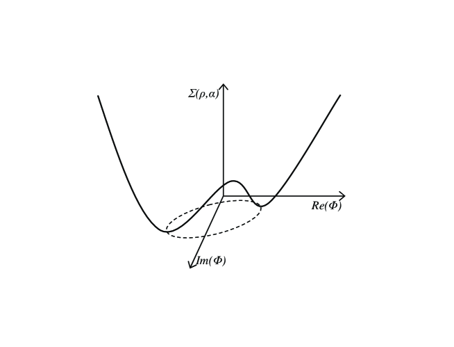
Figure 1: The function $\Sigma(\rho,\alpha)$, given in eq.(21), for external source module $r<r_{crit}$. The ’tilted Mexican hat’ shape possesses a valley of minima which define the semiclassical approximation.

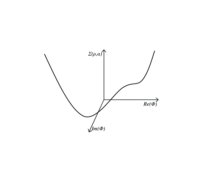
Figure 2: The function $\Sigma(\rho,\alpha)$, given in eq.(21), for external source module $r>r_{crit}$. The minima are located sharply around the $\cos(\alpha+\theta)=-1$ point. The second local minimum located at $\cos(\alpha+\theta)=1$ degenerates to an inflection point at $r=r_{crit}$ and disappears for $r>r_{crit}$.

2.4 Maxwell construction

As discussed in the previous subsection, in the case where $r<r_{crit}$ the partition function is dominated by:

$$Z[r] \simeq \int_{0}^{2\pi}\frac{d\alpha}{2\pi}\exp\left(-V\left[U_{bare}(\rho_{0})+2r\rho_{0}\cos(\alpha+\theta)\right]\right)$$

$$= \int_{0}^{2\pi}\frac{d\alpha}{2\pi}\exp\left(-V\left[U_{bare}(\rho_{0})+2r\rho_{0}\cos\alpha\right]\right)~{},$$

where $\rho_{0}$ depends on the source $r$ and is given by eq.(24). We note that the summation over all the points in the valley ensures that the partition function $Z$ depends on the modulus $r$ of the source only. After introducing the dimensionless quantities

$$A\equiv\lambda\frac{Vv^{4}}{24}~{}~{},~{}~{}\tilde{\rho}_{0}\equiv\frac{\rho_{0}}{v}~{}~{},~{}~{}\tilde{r}\equiv\frac{r}{r_{crit}}~{},$$ (28)

the minimum $\tilde{\rho}_{0}$ can be expanded in powers of $\tilde{r}$, and we find, up to fourth order,

$$\tilde{\rho}_{0}=1-\frac{\sqrt{3}}{9}\tilde{r}\cos\alpha-\frac{1}{18}(\tilde{r}\cos\alpha)^{2}-\frac{4\sqrt{3}}{243}(\tilde{r}\cos\alpha)^{3}-\frac{35}{1944}(\tilde{r}\cos\alpha)^{4}+{\cal O}(\tilde{r}^{5})~{}.$$ (29)

We obtain then

$$\exp\left(-V\left[U_{bare}(\rho_{0})+2r\rho_{0}\cos\alpha\right]\right)$$

$$= 1-\frac{8\sqrt{3}}{9}A\tilde{r}\cos\alpha+\frac{4}{27}A\left(1+8A\right)(\tilde{r}\cos\alpha)^{2}$$

$$+ \frac{4\sqrt{3}}{243}A\left(1-8A-\frac{64}{3}A^{2}\right)(\tilde{r}\cos\alpha)^{3}$$

$$+ \frac{8}{243}A\left(\frac{1}{3}-A+\frac{16}{3}A^{2}+\frac{64}{9}A^{3}\right)(\tilde{r}\cos\alpha)^{4}+{\cal O}(\tilde{r}^{6})~{},$$ (31)

and the integration over $\alpha$ leads finally to

$$Z(\tilde{r})=1+\frac{2A}{27}\left(1+8A\right)\tilde{r}^{2}+\frac{A}{81}\left(\frac{1}{3}-A+\frac{16}{3}A^{2}+\frac{64}{9}A^{3}\right)\tilde{r}^{4}+{\cal O}(\tilde{r}^{6})~{}.$$ (32)

This last expression will now be used to calculate the effective potential, around the origin.
From the definition (3) of the classical field, one finds

$$\rho_{c}=v\frac{3\sqrt{3}}{8AZ}\frac{\partial Z}{\partial\tilde{r}}~{},~{}~{}~{}~{}~{}\alpha_{c}=\pi-\theta~{},$$ (33)

such that the expansion (32) leads to

$$\tilde{\rho}_{c}\equiv\frac{\rho_{c}}{v}=\frac{\sqrt{3}}{18}\left(1+8A\right)\tilde{r}+\frac{\sqrt{3}}{81}\left(\frac{1}{2}-\frac{11}{6}A+\frac{8}{3}A^{2}-\frac{32}{3}A^{3}\right)\tilde{r}^{3}+{\cal O}(\tilde{r}^{5})~{}.$$ (34)

One can see that the regime $r<r_{crit}$ leads to a polynomial expansion of the classical field around $\rho_{c}=0$. We then invert the last series, by expanding $\tilde{r}$ in powers of $\tilde{\rho}_{c}$, and we find

$$\tilde{r}=\frac{18}{\sqrt{3}(1+8A)}~{}\tilde{\rho}_{c}+\frac{144\sqrt{3}(-1/2+11A/6-8A^{2}/3+32A^{3}/3)}{(1+8A)^{4}}~{}\tilde{\rho}_{c}^{3}+{\cal O}(\tilde{\rho}^{5})~{}.$$ (35)

Since $\Gamma=VU_{eff}$ is an increasing function of $\rho_{c}$, the equation of motion (8) can also be written

$$\left|\frac{\partial\Gamma}{\partial\tilde{\rho}_{c}}\right|=\frac{\partial\Gamma}{\partial\tilde{\rho}_{c}}=\frac{8A}{3\sqrt{3}}~{}\tilde{r}~{},$$ (36)

Together with the expansion (35), the integration over $\tilde{\rho}_{c}$ gives

$$\Gamma[\tilde{\rho}_{c}]=\frac{8A}{1+8A}\tilde{\rho}_{c}^{2}+\frac{48A(-1+11A/3-16A^{2}/3+64A^{3}/3)}{(1+8A)^{4}}\tilde{\rho}_{c}^{4}+{\cal O}(\tilde{\rho}_{c}^{6})~{},$$ (37)

where the constant of integration is disregarded. In the limit of large volume $A>>1$, the effective action is then

$$\Gamma[\rho_{c}]=\left(\frac{\rho_{c}}{v}\right)^{2}+\frac{1}{4}\left(\frac{\rho_{c}}{v}\right)^{4}+\cdots~{},$$ (38)

and the effective potential is finally obtained after dividing by the volume

$$U_{eff}(\rho_{c})=\frac{1}{V}\Gamma[\rho_{c}]=\frac{1}{V}\left(\frac{\rho_{c}}{v}\right)^{2}+\frac{1}{4V}\left(\frac{\rho_{c}}{v}\right)^{4}+\cdots~{}.$$ (39)

$U_{eff}$ therefore vanishes in the limit of infinite volume

$$U_{eff}(\rho_{c})\to 0~{}~{}~{}~{}\mbox{(infinite volume)}~{},$$ (40)

and has the form of a flat disc for $\rho_{c}<<v$. Few interesting remarks can be made here:

• This study has been done up to the 4th order in the classical field, but it is clear that the present construction can be extended to any order in $\rho_{c}$. Together with the convexity of the effective potential, proven in subsection 2.2, we expect the flatness to hold up to $\rho_{c}\simeq v$.

• The convexity of the potential (39) is actually valid for finite volume, and not only in the limit of infinite volume;

• The effective potential (39) is universal and does not depend on the bare self-coupling of the scalar field. This universality has been observed in exact Wilsonian renormalization group studies, where the Maxwell construction is obtained in the infrared limit of the so-called spinodal region [16]. In this region, the running potential is a universal quadratic function of the background field, independent of the details of the spontaneously broken ultraviolet potential.

To conclude this subsection, quantization of the theory erases the non-convex part of the bare potential, as expected from the general argument given in subsection 2.2, and verified within our semi-classical approximation.

2.5 Semi-classical partition function for $\rho_{c}>v$

In the situation where $r>r_{crit}$, there is no valley of saddle points anymore, but only one saddle point, which is obtained for $\cos(\alpha+\theta)=-1$, and it is easy to show that the semi-classical approximation leads to an effective potential which is identical to the bare potential, as we do here. The approximate partition function is

$$Z\simeq\exp\left(-V(U_{bare}(\rho_{0})-2r\rho_{0})\right)~{},$$ (41)

where $\rho_{0}$ is given by eq.(26). The classical field is therefore

$$\phi_{c}=\frac{-e^{-i\theta}}{2V}\frac{\partial(\ln Z)}{\partial r}=\frac{e^{-i\theta}}{2}\left[\left(\frac{dU_{bare}}{d\rho_{0}}-2r\right)\frac{d\rho_{0}}{dr}-2\rho_{0}\right]=e^{i(\pi-\theta)}\rho_{0}(r)~{},$$ (42)

such that

$$\rho_{c}=\rho_{0}(r)~{}~{}~{}~{}\mbox{and}~{}~{}~{}~{}\alpha_{c}=\pi-\theta~{}.$$ (43)

In the semi-classical approximation, the partition function can then be expressed as

$$Z=\exp\left(-V(U_{bare}(\rho_{c})-2r\rho_{c})\right)~{},$$ (44)

and, according to the result (43), the effective potential is finally

$$U_{eff}(\rho_{c})=-\frac{1}{V}\left(\ln Z+2Vr\rho_{c}\cos(\alpha_{c}+\theta)\right)=U_{bare}(\rho_{c})~{}.$$ (45)

Note that this result would also be obtained for a bare potential which does not feature spontaneous symmetry breaking. In that sense, the saddle point approximation (although non-perturbative in principle) constitutes a ’tree level’ approximation for potentials with a unique vacuum, or, far away from the degenerate vacua region. On the other hand, since it is sensitive to the presence of degenerate vacua, the saddle point summation captures a genuine non-perturbative effect which is the flattening of the potential within the disc of $\rho_{c}<v$. The smooth matching of the potential at $\rho_{c}\sim v$ between the flat disc and the convex outer branch would of course require a full non-perturbative calculation, currently possible only via Lattice Field Theory techniques.

3 Effective Potential for $O(N)$-symmetric theories

3.1 Convexity of the Effective Potential

It is straightforward to generalize the results of the previous section to scalar theories with a global $O(N)$ symmetry. For the N-plet of fields $\vec{\phi}=(\phi_{1},\phi_{2},\dots,\phi_{N})$ the action reads in Euclidean space

$$S[\vec{\phi}]=\int d^{4}x\left\{\frac{1}{2}\partial_{\mu}\vec{\phi}\cdot\partial_{\mu}\vec{\phi}+\frac{\lambda}{4}\left(\rho^{2}-v^{2}\right)^{2}\right\}~{},$$ (46)

where $\rho=\sqrt{\vec{\phi}\cdot\vec{\phi}}$. The partition function is

$$Z[\vec{j}]=\int{\cal D}[\vec{\phi}]~{}\exp\left(-S[\vec{\phi}]-\int_{x}\vec{j}\cdot\vec{\phi}\right)~{},$$ (47)

where $\vec{j}$ is the $O(N)$ vector source coupled to the fields. $Z$ and the connected graphs generating functional $W=-\ln Z$ depend only on the modulus $r=|\vec{j}|$ of the source vector as a consequence of the $O(N)$ invariance of the action and the integration measure ${\cal D}\vec{\phi}$. The classical field $\vec{\phi_{c}}$ is defined via

$$\vec{\phi}_{c}=-\frac{1}{Z}\frac{\delta Z}{\delta\vec{j}}=\frac{\delta W}{\delta\vec{j}}=\frac{\vec{j}}{r}~{}\frac{\delta W}{\delta r}~{},$$ (48)

and therefore its modulus $\rho_{c}=|\vec{\phi}_{c}|$ is

$$\rho_{c}=\frac{1}{Z}\left|\frac{\delta Z}{\delta r}\right|~{}.$$ (49)

The effective action is defined via the Legendre transform

$$\Gamma[\vec{\phi}_{c}]=W[r]-\int_{x}\vec{j}\cdot\vec{\phi}_{c}~{},$$ (50)

such that

$$\frac{\delta\Gamma}{\delta\vec{\phi}_{c}}=-\vec{j}~{}~{}~{}~{}~{}{\rm and}~{}~{}~{}~{}~{}\left|\frac{\delta\Gamma}{\delta\rho_{c}}\right|=r~{}.$$ (51)

The generating functional $W$ is concave, which can be shown as follows. We define the $N\times N$ operator with matrix elements

$$\left(\delta^{2}W\right)^{ab}\equiv\frac{\delta^{2}W}{\delta j_{a}\delta j_{b}}=\frac{\delta\phi_{c}^{a}}{\delta j_{b}}=\phi_{c}^{a}\phi_{c}^{b}-\left<\phi^{a}\phi^{b}\right>$$ (52)

where $\left<\dots\right>$ denotes an expectation value with respect to the partition function (47). Since $-\delta^{2}W$ coincides with the covariance matrix for the N-plet of fields $\vec{\phi}$, it has the general property of being a positive semi-definite matrix, with eigenvalues greater than zero. Following the steps in section 2, the convexity of $\Gamma$ arises from the examination of the operator $\delta^{2}\Gamma$ with matrix elements

$$\left(\delta^{2}\Gamma\right)_{ab}\equiv\frac{\delta^{2}\Gamma}{\delta\phi_{c}^{a}\delta\phi_{c}^{b}}=-\frac{\delta j_{a}}{\delta\phi_{c}^{b}}~{},$$ (53)

since

$$\delta^{2}W\cdot\delta^{2}\Gamma=-{\bf 1}{\bf{1}}~{},$$ (54)

where ${\bf 1}{\bf{1}}$ denotes the $N\times N$ unit matrix. For the effective potential $U_{eff}(\rho_{c})$ we consider constant field configurations such that

$$\frac{\delta^{2}}{\delta\phi_{c}^{a}\delta\phi_{c}^{b}}\int d^{4}x~{}U_{eff}(\rho_{c})=\left[\frac{U^{\prime}_{eff}}{\rho_{c}}~{}\delta^{ab}+\left(U_{eff}^{\prime\prime}-\frac{U^{\prime}_{eff}}{\rho_{c}}\right)\frac{\phi_{c}^{a}\phi_{c}^{b}}{\rho_{c}^{2}}\right]\delta^{4}(x-y)~{}.$$ (55)

Algebraically it is straightforward to check that an $N\times N$ real matrix of the form

$$M^{ab}=A~{}\delta^{ab}+B~{}n^{a}n^{b}~{}~{}~{},~{}{\rm with}~{}~{}~{}\sum_{a=1}^{N}n^{a}n^{a}=1~{},$$ (56)

possesses the eigenvalues

$$\lambda_{1}=\lambda_{2}=\dots=\lambda_{N-1}=A~{}~{}~{}{\rm and}~{}~{}\lambda_{N}=A+B~{}.$$ (57)

The convexity of $\Gamma$ therefore guarantees that

$$U^{\prime}_{eff}(\rho_{c})\geq 0~{}~{}~{}{\rm and}~{}~{}~{}U^{\prime\prime}_{eff}(\rho_{c})\geq 0~{},$$ (58)

and the effective potential is an increasing and convex function of $\rho_{c}$.

3.2 Maxwell Construction

The semiclassical approximation to the partition function (47) consists of summing over the minima of the functional

$$\Sigma[\vec{\phi}]=S[\vec{\phi}]+\int_{x}\vec{j}\cdot\vec{\phi}~{}.$$ (59)

For the effective potential it suffices to consider constant field configurations and minimize the function

$$\Sigma[\rho,\omega]=V\left[\frac{\lambda}{4}\left(\rho^{2}-v^{2}\right)^{2}+r\rho\cos\omega\right]~{},$$ (60)

where $\omega$ is the angle $(0\leq\omega\leq\pi)$ between $\vec{j}$ and $\vec{\phi}$ in field space. Thus, we search for the real and positive solutions $\rho_{0}$ of

$$\lambda(\rho^{2}_{0}-v^{2})\rho_{0}=-r\cos\omega~{}.$$ (61)

and the analysis presented in subsection (2.3) holds for a critical source modulus now taking the value

$$r_{crit}=\frac{2\lambda v^{3}}{3\sqrt{3}}~{}.$$ (62)

For $r\leq r_{crit}$, $\Sigma$ takes the shape of a ’tilted Mexican-hat potential’ with the minima given by

$$\rho_{0}=\frac{2v}{\sqrt{3}}\cos\left\{\frac{\pi}{3}-\frac{1}{3}\arccos\left(\frac{r}{r_{crit}}\cos\omega\right)\right\}~{}.$$ (63)

and the saddle point approximation consists of integrating over the $N-$ dimensional solid angle $\Omega_{N-1}$, which covers the valley of radial minima $\vec{\phi}^{2}=\rho_{0}^{2}$ in field space:

$$Z[r]\simeq\int\frac{d\Omega_{N-1}}{\Omega_{N-1}}\exp\left(-\Sigma[\rho_{0},\omega]\right)~{}.$$ (64)

Rescaling variables as

$$A\equiv\lambda\frac{Vv^{4}}{4}~{}~{},~{}~{}\tilde{\rho}_{0}\equiv\frac{\rho_{0}}{v}~{}~{},~{}~{}\tilde{r}\equiv\frac{r}{r_{crit}}~{},$$ (65)

we obtain, as in the complex scalar case,

$$\exp(-\Sigma[\rho_{0},\omega]) = 1-\frac{8\sqrt{3}}{9}A\tilde{r}\cos\omega+\frac{4}{27}A\left(1+8A\right)(\tilde{r}\cos\omega)^{2}$$

$$+ \frac{4\sqrt{3}}{243}A\left(1-8A-\frac{64}{3}A^{2}\right)(\tilde{r}\cos\omega)^{3}$$

$$+ \frac{8}{243}A\left(\frac{1}{3}-A+\frac{16}{3}A^{2}+\frac{64}{9}A^{3}\right)(\tilde{r}\cos\omega)^{4}+{\cal O}(\tilde{r}^{6})~{}.$$

Using the $O(N)$ invariance of $Z$ in the internal space, we can rotate $\vec{j}$ on the $N-$th axis such that $\omega$ becomes the polar angle of $\vec{\phi}$ with the $N-$th axis, thus effectively reducing

$$\frac{d\Omega_{N-1}}{\Omega_{N-1}}~{}\longrightarrow~{}\frac{d\omega}{I_{N-2}}(\sin\omega)^{N-2}~{}~{},~{}\mbox{with}~{}0\leq\omega\leq\pi~{},$$ (67)

where we define

$$I_{n}=\int_{0}^{\pi}d\omega(\sin\omega)^{n}~{}.$$ (68)

These integrals satisfy

$$I_{n}=\frac{n-1}{n}I_{n-2}~{},$$ (69)

and the calculation of the partition function involves only the even powers of $\cos\omega$ in the expression (3.2):

$$\int d\omega(\sin\omega)^{N-2} = I_{N-2}$$ (70)

$$\int d\omega(\sin\omega)^{N-2}\cos^{2}\omega = I_{N-2}-I_{N}=\frac{I_{N-2}}{N}$$

$$\int d\omega(\sin\omega)^{N-2}\cos^{4}\omega = I_{N-2}-2I_{N}+I_{N+2}=\frac{3I_{N-2}}{N(N+2)}~{}.$$

As a consequence, the partition function is

$$Z(\tilde{r})=1+\frac{4A}{27N}\left(1+8A\right)\tilde{r}^{2}+\frac{8A}{81N(N+2)}\left(\frac{1}{3}-A+\frac{16}{3}A^{2}+\frac{64}{9}A^{3}\right)\tilde{r}^{4}+{\cal O}(\tilde{r}^{6})~{}.$$ (71)

From the classical modulus (49), we find then

$$\tilde{\rho}_{c} \equiv \frac{\rho_{c}}{v}=\frac{3\sqrt{3}}{8AZ}\frac{\partial Z}{\partial\tilde{r}}=\frac{\sqrt{3}}{9N}\left(1+8A\right)\tilde{r}+$$

$$\frac{-4\sqrt{3}}{243N^{2}(N+2)}\left(-3N+2(1+5N)A+32(1-N)A^{2}+128A^{3}\right)\tilde{r}^{3}+{\cal O}(\tilde{r}^{5})~{},$$

and the corresponding expansion of $\tilde{r}$ in terms of $\tilde{\rho}_{c}$ reads

$$\tilde{r} = \frac{9N}{\sqrt{3}(1+8A)}~{}\tilde{\rho}_{c}+$$

$$\frac{12\sqrt{3}N^{2}}{(N+2)(1+8A)^{4}}(-3N+2(1+5N)A+32(1-N)A^{2}+128A^{3})~{}\tilde{\rho}_{c}^{3}+{\cal O}(\tilde{\rho}^{5})~{}.$$

Since $\Gamma=VU_{eff}$ is an increasing function of $\rho_{c}$, the equation of motion (51) can also be written

$$\left|\frac{\partial\Gamma}{\partial\tilde{\rho}_{c}}\right|=\frac{\partial\Gamma}{\partial\tilde{\rho}_{c}}=\frac{8A}{3\sqrt{3}}~{}\tilde{r}~{},$$ (74)

Together with the expansion (3.2), the integration over $\tilde{\rho}_{c}$ gives

$$\Gamma[\tilde{\rho}_{c}] = \frac{4NA}{1+8A}\tilde{\rho}_{c}^{2}$$

$$+\frac{8N^{2}A}{(N+2)(1+8A)^{4}}(-3N+2(1+5N)A+32(1-N)A^{2}+128A^{3})\tilde{\rho}_{c}^{4}+{\cal O}(\tilde{\rho}_{c}^{6})~{},$$

where the constant of integration is disregarded. Note that this result reproduces the effective action (37) when $N=2$. In the limit of large volume $A>>1$, the effective action is then

$$\Gamma[\rho_{c}]=\frac{N}{2}\left(\frac{\rho_{c}}{v}\right)^{2}+\frac{N^{2}}{4(N+2)}\left(\frac{\rho_{c}}{v}\right)^{4}+\cdots~{},$$ (76)

and the effective potential is finally obtained after dividing by the volume

$$U_{eff}(\rho_{c})=\frac{1}{V}\Gamma[\rho_{c}]=\frac{N}{2V}\left(\frac{\rho_{c}}{v}\right)^{2}+\frac{N^{2}}{4(N+2)V}\left(\frac{\rho_{c}}{v}\right)^{4}+\cdots~{}.$$ (77)

As in the complex scalar case, $U_{eff}$ vanishes in the limit of infinite volume

$$U_{eff}(\rho_{c})\to 0~{}~{}~{}~{}\mbox{(infinite volume)}~{},$$ (78)

and has the form of a flat $N$-ball for $\rho_{c}<v$. It is interesting to speculate about the large-$N$ limit of eq.(77). The first two terms of the series scale with $N/V$ at large-$N$, indicating a possible symmetry restoring vacuum (effective potential convex but not flat, with a minimum at $\rho_{c}=0$), if the large-volume and large-$N$ limit are taken simultaneously, with constant ratio $N/V$. In two dimensions, one may argue in favor of the existence of such a limit as symmetry breaking and massless Goldstone modes are prohibited by the Coleman-Mermin-Wagner theorem [17].

Finally, it is clear that for, $r>r_{crit}$, the unique minimum (26) of $\Sigma[\rho,\omega]$ dominates the partition function at the anti-alignment point $\cos\omega=-1$, and leads to an effective potential identical to the bare one. Such a result would also hold within the semiclassical approximation for a potential without SSB.

4 Remarks on the Abelian Higgs model

In this section, we demonstrate that, because of gauge fixing, no summation over the phase is involved in the semi-classical approximation for the partition function of the Abelian Higgs model. As a consequence, the presence of the gauge field does not allow the non-perturbative flattening of the scalar effective potential.
The Abelian Higgs model is described by the Lagrangian (Euclidean metric)

$$-\frac{1}{4}F_{\mu\nu}F^{\mu\nu}+D_{\mu}\phi(D^{\mu}\phi)^{\star}+U_{bare}(\rho)~{},$$ (79)

where $D_{\mu}=\partial_{\mu}-ieA_{\mu}$ and $U_{bare}$ is the standard SSB potential (19). The covariant derivative term can be written in terms of the modulus $\rho$ and argument $\alpha$ of the scalar field as

$$D_{\mu}\phi(D^{\mu}\phi)^{\star}=\partial_{\mu}\rho\partial^{\mu}\rho+\rho^{2}\partial_{\mu}\alpha\partial^{\mu}\alpha+e^{2}\rho^{2}A_{\mu}A^{\mu}-2e\rho^{2}A^{\mu}\partial_{\mu}\alpha~{}.$$ (80)

We then perform the gauge transformation

$$A_{\mu}\to A_{\mu}+e^{-1}\partial_{\mu}\alpha~{}~{},~{}~{}~{}~{}\phi\to\rho~{},$$ (81)

which eliminates completely the argument $\alpha$ from the theory

$$D_{\mu}\phi(D^{\mu}\phi)^{\star}=\partial_{\mu}\rho\partial^{\mu}\rho+e^{2}\rho^{2}A_{\mu}A^{\mu}~{}.$$ (82)

As a consequence, there is no summation over the scalar field argument, and the partition function is dominated by one saddle point only $(\rho=\mbox{const},A_{\mu}=0)$, leading to the argument similar to the one given in section 2.5. Therefore, based on the semi-classical approximation, the effective potential in the scalar sector remains identical to the bare one.
The reason why the convexity argument given in subsection (2.2) does not hold in this case is precisely gauge fixing, as we now explain. If one denotes $J^{\mu}$ the source for the gauge field, the corresponding classical fields of the theory are

$$A_{\mu}^{c}=\frac{\delta W}{\delta J^{\mu}}~{}\;\;\;,\;\;\;\phi_{c}=\frac{\delta W}{\delta j}~{}\;\;\;,\;\;\;\phi_{c}^{\star}=\frac{\delta W}{\delta j^{\star}}~{}\;,$$ (83)

and the connected graph generating functional $W$ will be a concave functional of the sources $j,j^{\star},J^{\mu}$. But in order to define the functional Legendre transform $\Gamma$, one needs to invert simultaneously the relations in (83) to express

$$\Gamma[\phi_{c},\phi^{\star}_{c},A_{\mu}^{c}]=W[j,j^{\star},J^{\mu}]-\int_{x}(j\phi_{c}+j^{\star}\phi^{\star}_{c}+J^{\mu}A_{\mu}^{c})~{},$$ (84)

where the sources are functionals of the classical fields. Since gauge symmetry relates locally the classical fields $A_{\mu}^{c},\phi_{c}$ and $\phi^{\star}_{c}$, this inversion is possible only after a choice of gauge, which reduces the space of fields, in order to have a one-to-one relation between sources and a gauge slice of classical fields. As a consequence, the operator

$$\delta^{2}\Gamma=\left(\begin{array}[]{ccc}\frac{\delta^{2}\Gamma}{\delta\phi_{c}^{\star}\delta\phi_{c}}&\frac{\delta^{2}\Gamma}{\delta\phi_{c}^{\star}\delta\phi_{c}^{\star}}&\frac{\delta^{2}\Gamma}{\delta\phi_{c}^{\star}\delta A_{\mu}^{c}}\\ \frac{\delta^{2}\Gamma}{\delta\phi_{c}\delta\phi_{c}}&\frac{\delta^{2}\Gamma}{\delta\phi_{c}\delta\phi_{c}^{\star}}&\frac{\delta^{2}\Gamma}{\delta\phi_{c}\delta A_{\mu}^{c}}\\ \frac{\delta^{2}\Gamma}{\delta\phi_{c}\delta A_{\nu}^{c}}&\frac{\delta^{2}\Gamma}{\delta\phi_{c}^{\star}\delta A_{\nu}^{c}}&\frac{\delta^{2}\Gamma}{\delta A_{\nu}^{c}\delta A_{\mu}^{c}}\end{array}\right)~{},$$ (85)

acts only on a sub-space of fields, compared to the operator

$$\delta^{2}W=\left(\begin{array}[]{ccc}\frac{\delta^{2}W}{\delta j\delta j^{\star}}&\frac{\delta^{2}W}{\delta j\delta j}&\frac{\delta^{2}W}{\delta j\delta J^{\mu}}\\ \frac{\delta^{2}W}{\delta j^{\star}\delta j^{\star}}&\frac{\delta^{2}W}{\delta j^{\star}\delta j}&\frac{\delta^{2}W}{\delta j^{\star}\delta J^{\mu}}\\ \frac{\delta^{2}W}{\delta j^{\star}\delta J^{\nu}}&\frac{\delta^{2}W}{\delta j\delta J^{\nu}}&\frac{\delta^{2}W}{\delta J^{\nu}\delta J^{\mu}}\end{array}\right)~{},$$ (86)

and cannot be its inverse anymore: the concave properties of $W$ do not lead to the convexity of $\Gamma$.
One can consider the following example, which shows the reduction of source space. If the source $\tilde{J}^{\mu}$ leads to the classical field $\tilde{A}_{\mu}^{c}$, we have

$$A_{\mu}^{c}=\frac{\delta W}{\delta J^{\mu}}=\int_{x}\frac{\delta W}{\delta\tilde{J}^{\nu}}\frac{\delta\tilde{J}^{\nu}}{\delta J^{\mu}}=\int_{x}\tilde{A}_{\nu}^{c}\frac{\delta\tilde{J}^{\nu}}{\delta J^{\mu}}~{}.$$ (87)

By choosing the specific relation

$$\tilde{J}^{\nu}=J^{\nu}+\theta\partial^{\nu}\partial_{\rho}J^{\rho}~{},$$ (88)

where $\theta$ is any scalar function with mass dimension -2, it is easy to see that $A_{\mu}^{c}$ and $\tilde{A}_{\mu}^{c}$ are related by the gauge transformation

$$A_{\mu}^{c}=\tilde{A}_{\mu}^{c}+\partial_{\mu}\Lambda~{}~{},~{}\mbox{with}~{}~{}\Lambda=\partial^{\rho}(\theta\tilde{A}_{\rho}^{c})~{}.$$ (89)

Therefore the use of both sources $J^{\mu}$ and $\tilde{J}^{\mu}$ leads to a redundancy of the classical fields, and $\tilde{J}^{\mu}$ should not be taken into account in the formal inversion of $\delta^{2}W$ which defines $\delta^{2}\Gamma$, if $J^{\mu}$ is already considered.
A complementary argument showing that one cannot prove convexity for the scalar effective potential is the following. One could naively think of integrating over the gauge field first, in the path integral of the Abelian Higgs model, in order to obtain an effective theory for the scalar field, such that the integration over the scalar field might lead to a convex effective potential. But the integration over the gauge field would actually generate a singular effective theory for the scalar field, in such a way that the convexity argument would not hold, because it is based on functional derivatives of $W$ and $\Gamma$. Indeed, in the above-mentioned gauge where the scalar field is real, the gauge sector of the bare Abelian Higgs Lagrangian is

$$A^{\mu}{\cal D}^{-1}_{\mu\nu}A^{\nu}~{},~{}~{}\mbox{with}~{}~{}{\cal D}^{-1}_{\mu\nu}=(\Box+e^{2}\rho^{2})\eta_{\mu\nu}-\partial_{\mu}\partial_{\nu}~{},$$ (90)

where the operator ${\cal D}^{-1}_{\mu\nu}$ is invertible for $\rho\neq 0$ only.
In order to quantize the model, one needs to choose a specific vacuum for the scalar field, and consider radial fluctuations around this vacuum, which are represented by a real scalar field. No Maxwell construction arises then, because the partition function is dominated by one minimum only, and the Higgs mechanism occurs as expected.

5 Conclusions

In this work we generalized the concept of Maxwell construction to scalar field theories with a continuous group symmetry possessing a non-trivial set of classical vacua. We demonstrated that the effective action is necessarily convex and, within a semiclassical approximation that takes into account all the degenerate space of non-trivial vacua, quantum fluctuations erase the non-convex part of the action. The result is a flat-disc shaped effective potential, for classical field values smaller than the vev of the system. We stress that it is crucial to first evaluate the partition function, and then perform the Legendre transform in order to arrive at this result. Thus, the vacuum of the quantized theory consists in a superposition of states with different field modulus, as a result of the absence of restoration force. This mechanism is the analogue of the coexistence of different phases for a statistical system, during a first order phase transition.
We noted that when the complex scalar is coupled to an Abelian gauge field and a Higgs mechanism is present, the convexity argument does not hold in general as the continuous set of vacua is eliminated by the gauge degrees of freedom.
The expression for the convex effective potential found in this work is independent of the coupling constant of the bare model, in the large volume limit, up to fourth order in the field at least, and depends only on the bare vev. This universality suggests that the construction presented here is independent of the details of the SSB bare potential.
A more complete study would involve a loop expansion around the dominant contributions which participate in the Maxwell construction. The flatness of the effective potential would certainly hold, since it appears to be the only way to satisfy convexity, if one starts with a SSB bare potential. The loop expansion would help determine the radius of convergence of the expansion in terms of the classical field, as well as the transition from the flat regime to the asymptotic classical form which occurs at values of the field modulus much larger than the vev.

Appendix: Maxwell construction for a real scalar field with SSB

The Maxwell construction presented in [7], for a real scalar field, is based on a weaker approximation than the one presented here: it takes into account the minimum of the bare potential only, not including the source term. The advantage of this approximation is the possibility to derive an analytical expression for the effective action, without the need for Taylor expansions in the classical field. As expected, the corresponding effective potential becomes flat in the limit of infinite volume. The drawback of the approximation in [7] is that the finite-volume expression for the effective action is not accurate, and only the infinite volume limit can be trusted. For the sake of completeness, we derive here the Maxwell construction for a real scalar field, using the more appropriate approximation described in the present article. We give only the main steps, which are similar to those detailed for the complex scalar field. As will be shown, the result coincides with the $O(N)$-symmetric model, with $N=1$, not only for infinite volume, but for any finite volume.
The SSB potential in the standard normalization is

$$U_{bare}(\phi)=\frac{\lambda}{24}(\phi^{2}-v^{2})^{2}~{},$$ (91)

and the partition function and classical field are

$$Z[j]=\int{\cal D}[\phi]\exp\left(-S[\phi]-\int_{x}j\phi\right)~{},~{}~{}\phi_{c}=-\frac{1}{Z}\frac{\delta Z}{\delta j}\to-\frac{1}{VZ}\frac{\partial Z}{\partial j}~{}.$$ (92)

This partition function is dominated by the two saddle points

$$\phi_{+}=\frac{2v}{\sqrt{3}}\cos\left\{\frac{\pi}{3}-\frac{1}{3}\arccos\left(\frac{j}{j_{crit}}\right)\right\}~{},\phi_{-}=\frac{2v}{\sqrt{3}}\cos\left\{\ \pi-\frac{1}{3}\arccos\left(\frac{j}{j_{crit}}\right)\right\}~{},$$ (93)

where

$$j_{crit}=\frac{\lambda v^{3}}{9\sqrt{3}}~{},$$ (94)

and $Z$ can be approximated by

$$Z[j]\simeq\frac{1}{2}\exp\left(-V[U_{bare}(\phi_{+})+j\phi_{+}]\right)+\frac{1}{2}\exp\left(-V[U_{bare}(\phi_{-})+j\phi_{-}]\right)~{}.$$ (95)

An expansion in powers of $j$ gives

$$Z=1+\frac{4A}{27}(1+8A)\tilde{j}+\frac{8A}{243}\left(\frac{1}{3}-A+\frac{16}{3}A^{2}+\frac{64}{9}A^{3}\right)\tilde{j}^{3}+\cdots~{},$$ (96)

where $A=\lambda Vv^{4}/24$ and dots represent higher orders in $\tilde{j}=j/j_{crit}$. The classical field is therefore given by

$$\frac{\phi_{c}}{v}\equiv\tilde{\phi}_{c}=-\frac{\sqrt{3}}{9}(1+8A)\tilde{j}-\frac{4\sqrt{3}}{729}(3-12A-128A^{3})\tilde{j}^{3}+\cdots~{},$$ (97)

and the inversion of this expansion gives

$$\tilde{j}=-\frac{3\sqrt{3}}{(1+8A)}\tilde{\phi}_{c}-\frac{4\sqrt{3}}{(1+8A)^{4}}(-3+12A+128A^{3})\tilde{\phi}_{c}^{3}+\cdots~{}.$$ (98)

The integration of the equation of motion

$$\frac{1}{V}\frac{\partial\Gamma}{\partial\phi_{c}}=-j~{},$$ (99)

gives the effective action $\Gamma$ as

$$\Gamma[\phi_{c}]=\frac{4A}{(1+8A)}\tilde{\phi}_{c}^{2}+\frac{8A}{3(1+8A)^{4}}(-3+12A+128A^{3})\tilde{\phi}_{c}^{4}+\cdots~{}.$$ (100)

Notice that this expression coincides with the effective action for the $O(N)$-symmetric model (Eq. 3.2) , when $N=1$ (taking into account the difference on the coupling $\lambda$ definition). At the large volume limit, we arrive at a form independent of the coupling:

$$\Gamma[\phi_{c}]\simeq\frac{1}{2}\left(\frac{\phi_{c}}{v}\right)^{2}+\frac{1}{12}\left(\frac{\phi_{c}}{v}\right)^{4}+\cdots~{}.$$ (101)

Finally, the effective potential is obtained after dividing by the volume $V$, and becomes flat in the limit $V\to\infty$.

References

- [1] K. Symanzik, Commun. Math. Phys. 16 (1970) 48; J. Iliopoulos, C. Itzykson and A. Martin, Rev. Mod. Phys. 47 (1975) 165.
- [2] R. W. Haymaker and J. Perez-Mercader, Phys. Rev. D 27 (1983) 1948.
- [3] Y. Fujimoto, L. O’Raifeartaigh and G. Parravicini, Nucl. Phys. B 212 (1983) 268.
- [4] V. A. Miransky, Singapore, Singapore: World Scientific (1993) 533 p
- [5] M. T. M. van Kessel, arXiv:0810.1412 [hep-ph].
- [6] L. O’Raifeartaigh, A. Wipf and H. Yoneyama, Nucl. Phys. B 271 (1986) 653.
- [7] J. Alexandre, Phys. Rev. D 86 (2012) 025028 [arXiv:1205.1160 [hep-th]].
- [8] R. Jackiw, Rev. Mod. Phys. 49 (1977) 681.
- [9] A. Rajantie and D. J. Weir, Phys. Rev. D 82 (2010) 111502 [arXiv:1006.2410 [hep-lat]].
- [10] R. Jackiw, Phys. Rev. D 9, 1686 (1974).
- [11] S. R. Coleman, R. Jackiw and H. D. Politzer, Phys. Rev. D 10 (1974) 2491.
- [12] L. F. Abbott, J. S. Kang and H. J. Schnitzer, Phys. Rev. D 13 (1976) 2212.
- [13] M. B. Halpern, Nucl. Phys. B 173 (1980) 504.
- [14] E. Brezin, J. C. Le Guillou and J. Zinn-Justin, In *Phase Transitions and Critical Phenomena, Vol.6*, Academic Press, London 1976, 125-247.
- [15] J. F. Donoghue, arXiv:1209.3511 [gr-qc].
- [16] C. Wetterich, Nucl. Phys. B 352 (1991) 529; J. Alexandre, V. Branchina and J. Polonyi, Phys. Lett. B 445 (1999) 351 [cond-mat/9803007]; D. F. Litim, J. M. Pawlowski and L. Vergara, hep-th/0602140; V. Pangon, S. Nagy, J. Polonyi and K. Sailer, Int. J. Mod. Phys. A 26 (2011) 1327 [arXiv:0907.0144 [hep-th]];
- [17] S. R. Coleman, Commun. Math. Phys. 31 (1973) 259; N. D. Mermin and H. Wagner, Phys. Rev. Lett. 17 (1966) 1133.