Electronic transport through ferromagnetic and superconducting junctions with spin-filter tunneling barriers.

Abstract

$\bar{t}$We present a theoretical study of the quasiparticle and subgap conductance of generic $X/I_{sf}/S_{M}$ junction with a spin-filter barrier $I_{sf}$, where $X$ is either a normal $N$ or a ferromagnetic metal $F$ and $S_{M}$ is a superconductor with a built-in exchange field. Our study is based on the tunneling Hamiltonian and the Green’s function technique. First, we focus on the quasiparticle transport, both above and below the superconducting critical temperature. We obtain a general expression for the tunneling conductance which is valid for arbitrary values of the exchange field and arbitrary magnetization directions in the electrodes and in the spin-filter barrier. In the second part we consider the subgap conductance of a normal metal-superconductor junction with a spin-filter barrier. We provide a heuristic derivation of new boundary conditions for the quasiclassical Green’s functions which take into account the spin-filter effect at interfaces. With the help of these boundary conditions, we show how the proximity effect and the subgap conductance are suppressed by spin-filtering in a $N/I_{sf}/S$ junction, where $N$ is a normal metal. Our work provides useful tools for the study of spin-polarized transport in hybrid structures both in the normal and in the superconducting state.

I Introduction

Over the last decade, there has been a growing interest in studying superconductor/ferromagnet ($S/F$) hybrid structures. On the one hand, this interest is due to the progress in technology that allows a controllable fabrication of nanohybrid structures using a wide range of superconducting and magnetic materials. On the other hand, this interest is due to the discovery of new and interesting fundamental phenomena, as for example the so-called $\pi-$state in $S/F/S$ junctions JosephsonBulaev77 ; Buzdin82 ; Ryaz ; Kontos ; Blum ; Bauer ; Sellier ; PalVolkovEfetov ; Weides09 , and more recently the long-range proximity effect mediated by odd-frequency triplet superconducting correlations in S/F structures BVE01 ; Kaizer06 ; Sosnin ; Birge ; Westerholt10 ; Chan ; BlamireScience ; Aarts (for an overview see Refs.GolubovRMP ; BuzdinRMP ; BVErmp ; EschrigPhysToday ; Zabel ).

The triplet superconducting correlations can carry spin-polarized supercurrents, i.e. currents without dissipation, that can be exploited in several ways in spintronics devicesEschrigPhysToday . In this context, the use of tunnel barriers with spin-dependent transmission, the so-called spin-filters, may be desirable for the creation of such spin supercurrents. Spin-filters are tunnel barriers with spin-dependent barrier height. They have been used for decades to generate polarized currents in spintronic circuits Moodera90 ; Moodera08 .

In spite of numerous works devoted to the theoretical study of $S/F$ structures, the study of the spin-filter effect in connection with the transport properties of S/F structures still remains open. For example, in Ref.Valles the transport properties of an S/F junction was calculated by using the Blonder-Tinkham-Klapwijk formalism Blonder . This analysis was extend in other several worksLinder ; Linder2 ; Fogelstrom2000 ; Kalenkov09 ; Tanaka97 ; Kawabata10 ; Belzig09 for S/F and S/F/S junctions in the ballistic and diffusive limit by taking into account spin-active interfaces between the F and S layersZaitsev84 ; Millis88 . In particular, the results for the diffusive limit presented in those works have been obtained by using the boundary conditions for the quasiclassical Green functions derived in Belzig09 . However, as we will show in section IV, these boundary conditions cannot describe the spin-filter effects and hence, none of the above mentioned works addressed the question how the spin-filtering affects the proximity effect in S/F structures. Only recently, we have analyzedBergeret12 the effect of spin filtering on the Josephson current through a $SF/I_{sf}/FS$ junction. It was shown that even in the case of a highly spin-polarizing barrier, a Josephson junction can flow provided the magnetizations of the F layers are non collinear. The results of Ref.Bergeret12 have been obtained from a model that combines the tunneling Hamiltonian and the quasiclassical Green’s functions, and provide a plausible explanation for a recent experiment on spin-filter Josephson junctionsBlamire . Note however, that the model used in Ref.Bergeret12 assumes exchange fields to be smaller than the Fermi energy and therefore cannot be straightforwardly generalized for the case of strong ferromagnets.

In the current paper, we present a general theory for the conductance through different hybrid structures with spin-filters as barriers, arbitrary values of the exchange field and arbitrary directions of the magnetization in the barrier and in the electrodes. We start with the model used in Ref.Bergeret12 and extend it to dissipative tunnel junctions. In the first part we focus on the study of the quasi-particle current and derive a general expression for the tunneling conductance. This expression recovers well known results in particular limiting cases and predicts new effects related to the mutual orientation of the magnetizations. We study the tunneling conductance of different junctions like $F/I_{sf}/F$, $HM/I_{sf}/HM$, and $F/I_{sf}/S$ ($HM$ stands for a ferromagnetic half-metal). In the second part we focus on the subgap transport through a $N/I_{sf}/S$ junction using the quasiclassical formalism. In order to quantify the effect of spin-filtering on the proximity effect we need to generalize the existing boundary conditionsK-L ; Belzig09 (BCs) for the quasiclassical equations. Accordingly, we present a heuristic derivation of new BCs which account for the spin-filter effect. These boundary conditions can be used in a wide range of problems involving superconductors, ferromagnets and spin-filter tunnel barriers. As an example, we study the subgap conductance of an $N/I_{sf}/S$ junction and show its suppression due to the spin-filter effect. Thus, our work provides on the one hand a new powerful tool for the theoretical study of spin transport in hybrid structures and on the other hand general expressions for the conductance that can be used for the interpretation of a broad range of experiments on spin transport through spin-filters.

II Model

We consider two type of junctions, first a generic tunnel junction $X_{l}/I_{sf}/X_{r}$ as the one shown in Fig. 1. The left and right electrodes, $X_{l}$ and $X_{r}$ are either ferromagnetic $F$ or a superconductor $S_{M}$ with a built-in exchange field $h$. The layer $I_{sf}$ is a spin-filter barrier, i.e., a spin-dependent tunneling barrier. The second type of junction we considered, is a $N/I_{sf}/S$ spin-filter junction between a normal metal ($N$) and a conventional superconductor ($S$). Our first aim is to derive a general expression for the current in both structures. For this purpose, we use the well known tunneling Hamiltonian method, which has been used in several works on tunneling in superconducting junctions (see the books KulikBook ; BaroneBook ; Schrieffer ; Wolf85 and references therein) and in systems with charge- and spin-density waves Artemenko83 ; Moor12 . The Hamiltonian consists of the Hamiltonians of the left (right) electrodes and the tunneling term

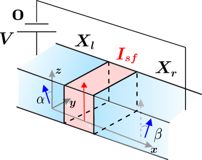
Figure 1: A generic tunnel junction $X_{l}/I_{sf}/X_{r}$. The left and right electrodes, $X_{l}$ and $X_{r}$, are either a ferromagnet $F$, normal metal $N$ or a superconductor $S_{M}$ with a built-in exchange field $h$. The layer $I_{sf}$ is a spin-filter barrier. $\alpha$ and $\beta$ are the orientation of the exchange field in the left and right electrodes.

$$H=H_{r}+H_{l}+H_{T}\;.$$ (1)

For the electrodes we consider the general Hamiltonian

$$H_{l}=\sum_{\mathbf{p},s}\xi_{\mathbf{p}}a_{\mathbf{p}s}^{\dagger}a_{\mathbf{p}s}+\sum_{\mathbf{p}}\left(\Delta a_{\mathbf{p}\uparrow}^{\dagger}a_{-\mathbf{p}\downarrow}^{\dagger}+h.c.\right)-\sum_{\mathbf{p},s,s^{\prime}}a_{\mathbf{p}s}^{\dagger}(h_{l}\mathbf{n.\hat{\sigma}})_{ss^{\prime}}a_{\mathbf{p}s^{\prime}},$$ (2)

where $a_{\mathbf{p}s}(a_{\mathbf{p}s}^{\dagger})$ is the annihilation (creation) operator of a particle with momentum $\mathbf{p}$ and spin $s$, $\xi_{\mathbf{p}}$ is the quasiparticle energy, $\Delta$ the superconducting gap, $\mathbf{\sigma}=(\sigma_{1},\sigma_{2},\sigma_{3})$ is a vector with the Pauli matrices, $h_{l}$ the amplitude of the effective exchange field and $\mathbf{n}$ a unit vector pointing in its direction. Similar Hamiltonian can be written for the right electrode.

The $H_{T}$ term in Eq. (1) describes the spin-selective tunneling through the spin-filter barrier $I_{sf}$ and is given by

$$H_{T}=\sum_{\{n,s,\mathbf{p,p}^{\prime}\}}\left(\mathcal{T}\hat{\sigma}_{0}+\mathcal{U}\hat{\sigma}_{3}\right)_{ss^{\prime}}a_{\mathbf{p}s}^{\dagger}b_{\mathbf{p}^{\prime}s^{\prime}}+h.c.$$ (3)

where $a$ and $b$ are the operators in the left and right electrodes respectively, $\mathcal{T}$ and $\mathcal{U}$ are the tunneling spin independent and spin dependent matrix elements, respectively. For simplicity we neglect the momentum dependence of $\mathcal{T}$ and $\mathcal{U}$, assuming that the characteristic energies are much smaller than the Fermi energy and that by tunneling the electrons are scattered randomly. The tunneling amplitude for spin up(down) is given by the relation: $T_{\uparrow(\downarrow)}=\mathcal{T}\pm\mathcal{U}$. The origin of the different tunneling amplitudes might be, for example, the conduction-band splitting in the ferromagnetic semiconducting barrier which leads to different tunnel barrier heights for spin-up and spin-down electrons Moodera90 ; Moodera08 .

In order to write the equation of motions for the Green’s functions it is convenient to write the tunneling Hamiltonian (3) in terms of new operators defined in an enlarged space (spin$\otimes$particle-hole). These operators are defined as:

$$A_{n,s}=\left\{\begin{array}[]{c}a_{s}\;\;{\text{f}or}\;\;n=1\\ a_{\bar{s}}^{\dagger}\;\;{\text{f}or}\;\;n=2\end{array}\right.$$ (4)

where $s=1,2$ is the spin up (down) index and $\bar{s}$ implies the change $1\leftrightarrow 2$. In analogy one introduces the operators $B_{n,s}$ for the right electrode. By using these operators the tunneling term (3) can be written as

$$H_{T}=\sum_{\{n,s,\mathbf{p,p}^{\prime}\}}[\check{A}_{\mathbf{p}}^{\dagger}\left(\mathcal{T}\hat{\tau}_{3}\otimes\hat{\sigma}_{0}+\mathcal{U}\hat{\tau}_{0}\otimes\hat{\sigma}_{3}\right)\check{B}_{\mathbf{p}^{\prime}}+h.c.]$$ (5)

where $\check{A}=A_{n,s}$ and $\check{B}=B_{n,s}$. The Hamiltonian (2) transforms to (see, for example, Ref.BVErmp )

$$H_{l}=\sum_{\{n,s,\mathbf{p}\}}\check{A}_{\mathbf{p}}^{\dagger}\mathcal{H}_{l}\check{A}_{\mathbf{p}},$$ (6)

with $\mathcal{H}_{l}=\xi_{\mathbf{p}}\hat{\tau}_{3}\otimes\hat{\sigma}_{0}+\left(\Delta\hat{\tau}_{1}\otimes\hat{\sigma}_{3}+h.c.\right)-h_{l}\hat{\tau}_{0}\otimes\hat{\sigma}_{3}$, for a exchange field directed along the $z$-axis. One can take into account an arbitrary direction of the exchange field (or magnetization vector) by means of a rotation in spin-space. We assume throughout this work that the transport takes place in the $x$-direction while the magnetization vector of the ferromagnets lies in the junction plane, i. e., the $(y,z)$-plane. A rotation in plane is described by the matrix

$$\check{R}_{\alpha}=\cos(\alpha/2)+i\hat{\tau}_{3}\otimes\hat{\sigma}_{1}\sin(\alpha/2)\;,$$ (7)

where $\alpha$ is the rotation angle.

In order to calculate the tunneling current through the generic junction, we first write the Dyson equation for the Keldysh Green’s functions $\check{G}_{l}$, for instance, in the left electrode

$$i\partial_{t}\check{G}_{l}=1+\check{\Sigma}_{l}\check{G}_{l}+\check{\mathcal{H}}_{l}\check{G}_{l}$$ (8)

Here $\check{\Sigma}_{l}=\sum_{\mathbf{q}}\check{\Gamma}\check{G}_{r}(\mathbf{q})\check{\Gamma}^{\dagger}$ is the self-energy partSchrieffer ; Volkov75 ; Artemenko83 ; Bergeret2005 ; Moor12 related to the tunnel Hamiltonian (5), $\check{G}_{r}$ is the full (non-quasiclassical) Green’s function in the right electrode and $\check{\Gamma}=\mathcal{T}\hat{\tau}_{3}\otimes\hat{\sigma}_{0}+\mathcal{U}\hat{\tau}_{0}\otimes\hat{\sigma}_{3}.$ In the following we restrict our analysis to the lowest order in tunneling. In this case the Green’s function $\check{G}_{l}$ is determined by Eq.(8) after neglecting the second term on the r.h.s. The exact form of $\check{G}_{l}$ is given in Eq.(12).

We proceed as usual subtracting from the Eq.(8) (prelimenary multiplied by $\hat{\tau}_{3}$ from the left) its conjugated equation multiplied by $\hat{\tau}_{3}$ from from the right:

$$i(\hat{\tau}_{3}\partial_{t}\check{G}+\partial_{t^{\prime}}\check{G}\hat{\tau}_{3})_{l}=\hat{\tau}_{3}\check{\Sigma}\check{G}-\check{\check{G}\check{\Sigma}\hat{\tau}_{3}+\hat{\tau}_{3}\check{G}\check{\mathcal{H}}_{l}-\mathcal{H}}_{l}\check{G}\hat{\tau}_{3}|_{l}\;.$$ (9)

If we now multiply the Keldysh component of this equation by the electron charge $e,$ set $t=t^{\prime}$, take the trace and sum up over momenta, we obtain on the l.h.s the time derivative of the charge, $\partial_{t}Q$. Thus, the current density $j$ through the barrier is then determined by the first two terms in the r.h.s.

$$I_{T}=-\frac{e}{32\pi}\sum_{\mathbf{p,q}}\int\frac{d\epsilon}{2\pi}\mathrm{Tr}\left\{\hat{\tau}_{3}\otimes\hat{\sigma}_{0}\left[\check{\Gamma}_{\alpha\beta}\check{G}_{r}(\mathbf{q},\epsilon)\check{\Gamma}_{\alpha\beta}^{\dagger},\check{G}_{l}(\mathbf{p},\epsilon)\right]^{K}\right\}$$ (10)

where $\check{\Gamma}_{\alpha\beta}\equiv\check{R}_{\alpha}^{\dagger}\check{\Gamma}\check{R}_{\beta}$, and we have defined $\check{\Gamma}$ after Eq.(8). The Green’s functions $\check{G}_{l,r}$ correspond to the case of the magnetization vector oriented parallel to the $z$-axis. We expressed the Green’s functions $\check{G}_{l\alpha}(\mathbf{p},\epsilon)$ for arbitrary magnetization orientation through the matrices $\check{G}_{l,r}$ as follows: $\check{G}_{l\alpha}(\mathbf{p},\epsilon)=\check{R}_{\alpha}\int d(t-t^{\prime})$ $\check{G}_{l0}(\mathbf{p},t-t^{\prime})\exp(i\epsilon(t-t^{\prime}))\check{R}_{\alpha}^{\dagger}.$

In the case that the energies involved in the problem are much smaller than the Fermi energy, one can perform the momentum integration in Eq.(10) and the current can be written in terms of quasiclassical Green’s functions $\check{g}_{l\alpha}=(i/\pi)\hat{\tau}_{3}\otimes\hat{\sigma}_{0}\int d\xi_{p}\check{G}_{l\alpha}(\mathbf{p},\epsilon)$

$$I_{T}R_{N}=[16e(\mathcal{T}^{2}+\mathcal{U}^{2})]^{-1}\int d\epsilon\mathrm{Tr}\left\{\hat{\tau}_{3}\otimes\hat{\sigma}_{0}\left[\mathit{\check{\Gamma}}_{\alpha\beta}\,\check{g}_{r}(\epsilon)\mathit{\check{\Gamma}}_{\alpha\beta}^{\dagger},\check{g}_{l}(\epsilon)\right]^{K}\right\}$$ (11)

where $\mathit{\check{\Gamma}}_{\alpha\beta}=\check{\Gamma}_{\alpha\beta}\hat{\tau}_{3}\otimes\hat{\sigma}_{0}.$ The resistance $R_{N}=[4\pi e^{2}N_{l}(0)N_{r}(0)(\mathcal{T}^{2}+\mathcal{U}^{2})]^{-1}$ is the junction resistance in the normal state, i. e., the resistance of an $F/I_{sf}/F$ junction with parallel orientation of magnetization along the $z$-axis, $N_{l,r}(0)=(p_{F}m/2\pi^{2})_{l,r}$ are the density of states (DOS) at the Fermi level. One should have in mind that by going over to the quasiclassical Green’s functions we lose the spin dependence of the DOS in the normal state. In that case the retarded (advanced) Green’s functions $\check{g}_{l,r}^{R(A)}$ in the ferromagnet have a trivial structure in spin-space, $\check{g}_{F}^{R(A)}=\pm\hat{\tau}_{3}\otimes\hat{\sigma}_{0}$, so that the normalized density of states is the same for spin up and down. This approach is valid for electrodes with small spin-splitting at the Fermi level, and was used for example in Ref.Bergeret12 for the calculation of the Josephson current through a $S/I_{sf}/S$ junction. However, if the spin-polarization of the electrodes at the Fermi level is large enough one has to use Eq.(10) in order to compute the current. This is done in the next section, where we calculate the conductance of a $F/I_{sf}/S_{M}$ and a $F/I_{sf}/F$ junction.

III The conductance for junctions with arbitrary exchange fields

In this section we consider junctions of the type $F/I_{sf}/F$ and $F/I_{sf}/S_{M}$, where F is a ferromagnet and $S_{M}$ describes either a thin $FS$ bilayerBergeret2001a or a superconductor with an induced spin-splitting field due to the proximity of the magnetic barrier $I_{sf}$Sauls88a . We are interested in arbitrary strength of exchange field and therefore we have to go beyond quasiclassics and use Eq. (10) for the current. We assume a bias voltage $V$ between the electrodes setting the electric potential in the superconducting electrode equal to zero (Fig. 1). In the tunneling limit the junction under consideration can only carry a normal (quasiparticle) current, which is determined by the normal Green’s functions $\check{G}_{l,r}$. These are diagonal in spin space with diagonal elements given by

$$\hat{G}_{r\pm}^{R}(\mathbf{p})=\frac{(\epsilon_{\pm}+i\gamma)\hat{\tau}_{0}+\xi_{\mathbf{p}}\hat{\tau}_{3}}{(\epsilon_{\pm}+i\gamma)^{2}-(\xi_{\mathbf{p}}^{2}+\Delta^{2})}\text{ }$$ (12)

where $\epsilon_{\pm}=\epsilon\pm h_{r},$ $\xi_{\mathbf{p}}=(p^{2}-p_{F,r}^{2})/2m_{r}$ and $\gamma$ is a damping in the excitation spectrum of the superconductor due to inelastic processes or due to coupling with the normal metal electrode. The corresponding Green’s function in the left ($F$) electrode has the same form if we set $\Delta=0$ and replace the index $r$ by $l$. As usual, the advanced Green’s function $G^{A}$ is defined in a similar way with the opposite sign of the damping term, $-i\gamma$. The full Green’s function in a superconductor has the form $\check{G}_{r}^{R}=\hat{G}_{r}^{R}\otimes\hat{\tau}_{0}+\hat{F}_{r}^{R}\otimes\hat{\tau}_{1},$ where $\hat{G}_{r}^{R}=G_{r0}^{R}\hat{\sigma}_{0}+G_{r3}^{R}\hat{\sigma}_{3},$ $G_{r0,3}^{R}=(G_{r+}^{R}\pm G_{r-}^{R})/2,$ and $\hat{F}_{r}^{R}$ is the anomalous (Gor’kov’s) Green’s function. Using the fact that the normal part of matrices $\check{G}_{r,l}$ are diagonal in the spin and particle-hole space, we can represent the current, Eq. (10) in the form

$$I_{T}=\frac{\pi e}{2}[(N_{n\uparrow}+N_{n\downarrow})_{l}(N_{n\uparrow}+N_{n\downarrow})_{r}]\int d\epsilon n_{V}(\epsilon)\mathrm{Tr}\left\{\hat{\tau}_{0}\otimes\hat{\sigma}_{0}\left[\check{\Gamma}_{\alpha\beta}\,\check{\nu}_{l}(\epsilon)\check{\Gamma}_{\alpha\beta}^{\dagger}\,\check{\nu}_{r}(\epsilon)\right]\right\}$$ (13)

where $n_{V}(\epsilon)=\{\tanh[(\epsilon+eV)/2T]-\tanh[(\epsilon-eV)/2T]\}/2,$ and $T$ is the temperature. The matrices $\check{\nu}_{l,r}(\epsilon)$ are related to $\hat{G}_{r\pm}^{R}(\mathbf{p})$ via $\check{\nu}(\epsilon)=(i/2\pi){(N_{0\uparrow}+N_{0\downarrow})}^{-1}\sum_{\mathbf{p}}[\check{G}^{R}(\mathbf{p})-\check{G}^{A}(\mathbf{p})]$, and can be written in the form: $\check{\nu}_{l,r\pm}(\epsilon)=[\nu_{0}(\epsilon)\hat{\tau}_{0}\otimes\hat{\sigma}_{0}+\nu_{3}(\epsilon)\hat{\tau}_{3}\otimes\hat{\sigma}_{3}]_{l,r}$ with $\hat{\nu}_{0,3}(\epsilon)=[\hat{\nu}(\epsilon+h)\pm\hat{\nu}(\epsilon-h)]/2$. It is useful to write the coefficients $\nu_{0,3}(\epsilon)$ in terms of of the DOS for spin up and down, $N_{\uparrow,\downarrow}$: $\nu_{0,3}=(N_{\uparrow}\pm N_{\downarrow})/(N_{n\uparrow}+N_{n\downarrow})$, where $N_{n\uparrow,\downarrow}(0)$ are the DOS at the Fermi level in the normal state of ferromagnets. The matrices $\check{\Gamma}_{\alpha\beta}$ which describe the tunneling probability are given by

$$\check{\Gamma}_{\alpha\beta}=\mathcal{T}\hat{\tau}_{3}\otimes\hat{\sigma}_{0}\cos(\frac{\alpha-\beta}{2})+\mathcal{U}\hat{\tau}_{0}\otimes\hat{\sigma}_{3}\cos(\frac{\alpha+\beta}{2})+i\mathcal{T}\hat{\tau}_{0}\otimes\hat{\sigma}_{1}\sin(\frac{\alpha-\beta}{2})-\mathcal{U}\hat{\tau}_{3}\otimes\hat{\sigma}_{2}\sin(\frac{\alpha+\beta}{2})$$ (14)

Substituting these expressions into Eq.(13), we find for the normalized conductance

$$\mathit{G}_{\alpha\beta}(V)\equiv R_{F}dI_{T}/dV=(1/2e)\int d\epsilon(dn_{V}/dV)Y_{\alpha\beta}(\epsilon)\;,$$ (15)

where the spectral conductance $Y_{\alpha\beta}(\epsilon)$ is defined as

$$Y_{\alpha\beta}(\epsilon)=\{\nu_{0l}\nu_{0r}+\frac{[\mathcal{T}^{2}\cos(\alpha-\beta)+\mathcal{U}^{2}\cos(\alpha+\beta)]}{(\mathcal{T}^{2}+\mathcal{U}^{2})}\nu_{3l}\nu_{3r}+2\frac{\mathcal{TU}}{(\mathcal{T}^{2}+\mathcal{U}^{2})}\mathcal{[}\nu_{0l}\nu_{3r}\cos\beta+\nu_{3l}\nu_{0r}\cos\alpha]\}\;.$$ (16)

and the resistance $R_{F}$ is defined as $R_{F}=[\pi e^{2}(N_{n\uparrow}+N_{n\downarrow})_{l}(N_{n\uparrow}+N_{n\downarrow})_{r}]^{-1}.$

Equations (15-16) are one of the main results of the present paper. They determine the conductance of the generic junction of Fig. 1 in a quite general situation, since they are valid for arbitrary exchange field, spin-filter strength and angles $\alpha$ and $\beta$. At low temperatures ($T\ll\Delta$) one can evaluate the energy integral in Eq. (15) obtaining a simple expression for the normalized conductance

$$\mathit{G}_{\alpha\beta}(V)=\frac{Y_{\alpha\beta}(eV)+Y_{\alpha\beta}(-eV)}{2}\;.$$ (17)

We now proceed to consider different types of junctions and calculate the conductance with the help of the last expressions.

III.1 Junctions with non-superconducting electrodes

Let us first consider junctions in the normal state. For example in a $N/I_{sf}/F$ junction the left electrode is a normal metal with no spin-polarization, therefore $\nu_{3}=0$ and $\nu_{0}=1$. From Eq.(LABEL:Y(V)Sp) we then obtain

$$Y_{\alpha\beta}^{(NF)}=1+P_{b}P_{r}\cos\beta\;,$$ (18)

where we have defined the polarization of the electrodes as $P_{l(r)}=(N_{\uparrow,l(r)}-N_{\downarrow,l(r)})/(N_{\uparrow,l(r)}+N_{\downarrow,l(r)})$. We have also introduced the quantity $P_{b}=2\mathcal{TU}/((\mathcal{T}^{2}+\mathcal{U}^{2}))=(T_{\uparrow}^{2}-T_{\downarrow}^{2})/(T_{\uparrow}^{2}+T_{\downarrow}^{2})$, which is a measure for the spin-filter efficiency. The quantity $P_{b}$ equals zero for spin-independent transmission coefficient and equals one for a 100% spin-filter effect. Eq. (18) shows that in the presence of a spin-filtering effect ($P_{b}\neq 0$), the conductance depends on the relative angle $\beta$ between the magnetizations of the F electrode and the spin-filter barrier.

In the case of a $F/I_{sf}/F$ junction we obtain a general expression for the spectral conductance

$$Y_{\alpha\beta}^{(FF)}=1+P_{l}P_{r}\frac{[\mathcal{T}^{2}\cos(\alpha-\beta)+\mathcal{U}^{2}\cos(\alpha+\beta)]}{(\mathcal{T}^{2}+\mathcal{U}^{2})}+P_{b}{[}P_{r}\cos\beta+P_{l}\cos\alpha]\;,$$ (19)

In order to make a connection with the effect of tunnel magnetoresistance we define the relative conductance change as

$$TMR=\frac{G_{00}-G_{0\pi}}{G_{0\pi}}\;.$$ (20)

Thus, for the $F/I_{sf}/F$ junction one obtains

$$TMR=2\frac{P_{r}(P_{l}+P_{b})}{1-P_{r}(P_{l}+P_{b})+P_{b}P_{l}}\;.$$ (21)

If we assume that there is no spin-filter, i.e. $P_{b}=0$ then Eq. (21) leads to the well-know Julliere’s formula Julliere .

Now we consider ferromagnetic electrodes with collinear magnetizations. We distinguish two magnetic configurations: the parallel one P, i.e $\beta=\alpha$ and the antiparallel configuration AP, $\beta=\alpha+\pi$.

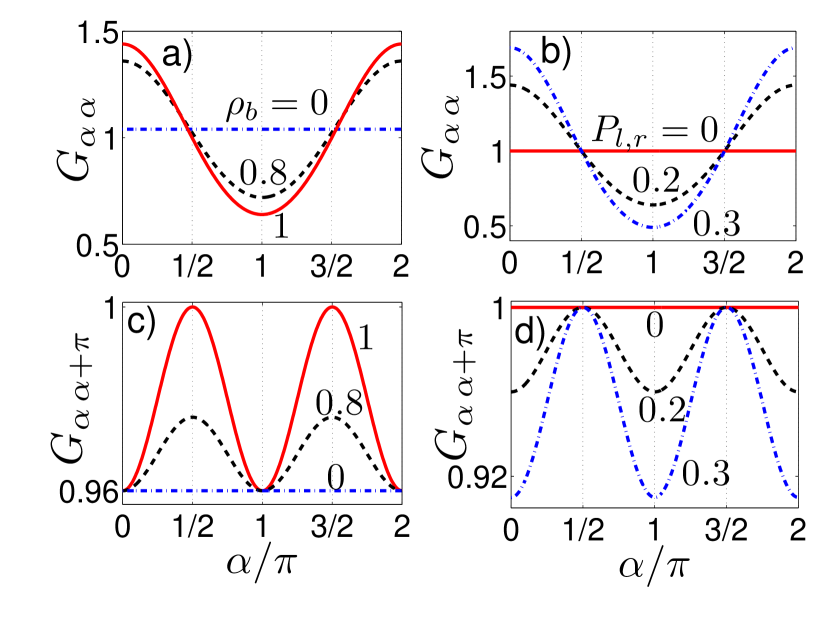
Figure 2: The normalized conductance $G_{\alpha,\beta}$ for a $F_{l}/I_{sf}/F_{r}$ junction as a function of the magnetization orientation. Panel (a): the parallel (P) configuration (i.e $\beta=\alpha$). Panel (b): the antiparallel (AP) configuration ($\beta=\alpha+\pi$). The polarizations in the left (right) electrodes $P_{l,r}$ are:$P_{l}=P_{r}=0.2$ (panels (a) and (c)). The parameter characterizing the spin-dependent barrier transmission $P_{b}$ equals $P_{b}=1$ (panels (b) and (d)).

In Fig.(2) we show the conductance of a junction with $P_{l}=P_{r}$ in these two cases. In the P configuration the conductance is $2\pi$-periodic and, depending on the angle $\alpha$, it is larger or smaller than in the non magnetic case. The largest value of the conductance is obtained when the magnetizations of the electrodes and the barrier are parallel. In the AP configuration the conductance is $\pi$-periodic and it is always smaller than in the non magnetic case. It is interesting to note that in the case of a fully polarizing barrier $P_{b}=1$ and perpendicular magnetization of the ferromagnets with respect to $I_{sf}$ ($\alpha=\pi/2$), the conductance equals 1 of a non-magnetic junction for arbitrary value of the spin-polarization of the electrodes and for both configurations P and AP (see panels (b) and (d) in Fig.(2)).

If the junction consists of two half-metallic ferromagnets (HM) then $P_{l,r}=1$ and from Eq. (19) one obtains

$$Y_{\alpha\beta}^{(HM)}=1+\frac{[\mathcal{T}^{2}\cos(\alpha-\beta)+\mathcal{U}^{2}\cos(\alpha+\beta)]}{(\mathcal{T}^{2}+\mathcal{U}^{2})}+P_{b}{[}\cos\beta+\cos\alpha]\;,$$ (22)

It is clear from this expression that the conductance of a non-magnetic barrier ($\mathcal{U}=0$) vanishes if the magnetizations of the left and right electrodes are antiparallel ($\beta=\alpha+\pi$).

If $\alpha=\beta=0$ and $\alpha=\beta=\pi,$ the spectral conductance is given by

$$Y_{00,\pi\pi}^{(HM)}=2(1\pm P_{b})$$ (23)

As expected, the conductance of the $HM/I_{sf}/HM$ junction with a barrier impenetrable for one spin direction vanishes if the magnetization in the left and right electrodes are antiparallel with respect to the magnetization of the barrier.

III.2 Junctions with one superconducting electrode

We consider now a $F/I_{sf}/S$ junction and calculate the conductance of the system using Eqs. (15-LABEL:Y(V)Sp). In the superconducting electrode $\nu_{0,3,r}(\epsilon)=[\nu_{r}(\epsilon+h_{r})\pm\nu_{r}(\epsilon-h_{r})]/2$, where $\nu_{r}(\epsilon)=\epsilon/\sqrt{\epsilon^{2}-\Delta^{2}}$. Here $h_{r}$ is an effective exchange field induced in the superconductor by the proximity of a thin F-layer (as in a $F/I_{sf}/FS$ junction) or by the proximity of the magnetic barrier $I_{sf}$ itself Sauls88a . In this case $\nu_{0l}$, $\nu_{0r}$ and $\nu_{3l}$ are even functions of $\epsilon$ and $\nu_{3r}$ is an odd functions of $\epsilon$ (in the quasiclassical approximation). Only the first and last terms of Eq. (LABEL:Y(V)Sp) contribute to the integral in Eq. (15). Thus, the spectral conductance $Y_{\alpha\beta}(\epsilon)$ can be written as follows

$$Y_{\alpha\beta}(\epsilon)^{(FS)}=\nu_{0r}\left(1+P_{b}P_{l}\cos\alpha\right)\;.$$ (24)

This equation, as well as Eq. (LABEL:Y(V)Sp), resembles the Slonczewski formulaSlonczewski . It generalizes the latter for the case of a superconducting electrode and a spin-filter barrier.

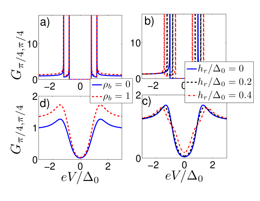
Figure 3: The voltage dependence of the ratio $\tilde{G}=G_{\pi/4,\pi/4}/G_{0}$, where $G_{\pi/4,\pi/4}$ is the normalized conductance for a $F/I_{sf}/S_{M}$ junction with fixed polarization in the ferromagnetic electrode ($P_{l}=0.5$) and fixed angles ($\alpha=\beta=\pi/4$), and $G_{0}$ is the normalized conductance for a $F/I_{sf}/S_{M}$ junction with zero polarization in the ferromagnetic electrode ($P_{l}=0$), zero exchange field in the superconductor ($h_{r}=0$) and no spin-filter effect ($P_{b}=0$). In panels (a) and (b) at zero temperature and in panels (c) and (d) at $T=0.2T_{c}^{0}$, where $T_{c}^{0}$ is the critical temperature for $h_{r}=0$. In panel (a) $h_{r}=0.2\Delta_{0}$ and $P_{b}=0,1$. In panel (b) $h_{r}=0,0.2,0.4\Delta_{0}$ and $P_{b}=0.8$. In panel (c) $h_{r}=0.2\Delta_{0}$ and $P_{b}=0,0.8,1$. In panel (d) $h_{r}=0,0.2,0.4\Delta_{0}$ and $P_{b}=0.8$. By calculating the curves we have added a small $\gamma=0.01\Delta_{0}$ damping factor.

In Fig.3 we show the conductance for the $F/I_{sf}/S$ junction obtained from Eqs. (15, 24). One can see the splitting of the conductance peaks at $eV=\pm\Delta\pm h_{r}$ due to the finite exchange field $h_{r}$ in the superconducting electrode. Note that by increasing the temperature the peaks smeared out and are more difficult to recognize. From Figs 3a and 3c one can see that the values of $G$ in the normal state, i.e. the asymptotic values for $V\gg\Delta$, depends on the polarization of the barrier, in accordance with Eq. (18).

IV Subgap Conductance in $N/I_{sf}/S$ Junctions: Effective Boundary Conditions

In the previous sections we have calculated the conductance of different junctions in the tunneling limit. In other words, the Green’s functions in the left and right electrodes have not been corrected due to the proximity effect. However, it is well known that the proximity effect in $N/S$ structures induces a condensate in the normal metal which causes a subgap conductance in $N/S$ junctions Kastalsky91 ; Quirion02 . In order to quantify the proximity effect we need boundary conditions that take into account the spin-filtering at the $N/S$ barrier. Surprisingly, in spite of many works on $N/S$ and $F/S$ structures such boundary conditions are absent in the literature Zaitsev84 ; Shelankov84 ; Millis88 ; Tanaka97 ; Eschrig2000 ; Fogelstrom2000 ; Belzig09 ; Kalenkov09 ; Kawabata10 . In order to fill this gap we present here a heuristic derivation of the boundary conditions at $S_{M}/I_{sf}/S_{M}$ interface which can also be used for $N/I_{sf}/S$ or $S/I_{sf}/FS$ interfaces.

We consider the diffusive limit and write down the Usadel-like equation for the Keldysh function $\check{g}^{K}$ in the $S_{M}$ electrodes

$$-D\partial_{x}(\check{g}\partial_{x}\check{g})^{K}-[i\hat{\tau}_{3}\otimes(\hat{\sigma}_{0}\epsilon-\hat{\sigma}_{3}h(x))+\Delta\hat{\tau}_{2}\otimes\hat{\sigma}_{3},\check{g}^{K}]=0$$ (25)

We assume that the exchange field $h$ differs from zero only in a thin enough layer of thickness $d_{F}\ll\xi_{h}$. This allows us to integrate Eq.(25) over the thickness $d_{F}$ considering the Green’s functions $\check{g}^{K}$ to be constant in this narrow layer. Performing this procedure at $x>0$, we obtain for the ”spectral” matrix current $\check{I}^{K}(\epsilon)$

$$\check{I}^{K}(\epsilon)\equiv(\check{g}\partial_{x}\check{g})^{K}|_{x=d_{F}}=i\kappa_{h}[\hat{\tau}_{3}\otimes\hat{\sigma}_{3},\check{g}_{r(l)}]+\check{I}_{T}^{K}\text{ }$$ (26)

where $\kappa_{h}=hd_{F}/D$. The latter term describes the tunneling current. The charge current density, for example, in the right superconductor is given by

$$I=(\sigma_{r}/16e)\int d\epsilon\mathrm{Tr}\left\{\hat{\tau}_{3}\otimes\hat{\sigma}_{0}[\check{g}_{r}\partial_{x}\check{g}_{r}]^{K}\right\}$$ (27)

This current equals the tunneling current given in (11). Therefore one can assume that

$$\check{I}_{T}^{K}=\text{ }\frac{\kappa_{T}}{\mathcal{T}^{2}+\mathcal{U}^{2}}\left[\mathit{\check{\Gamma}}_{\alpha\beta}\,\check{g}_{l}\mathit{\check{\Gamma}}_{\alpha\beta}^{\dagger},\check{g}_{r}\right]^{K}$$ (28)

where $\kappa_{T}=1/(\sigma_{r}R_{N\Box})$, $\sigma_{r}$ is the conductivity of the right $S$ electrode in the normal state, and $R_{N\Box}$ is the interface resistance in the normal state per unit area.

Equations (26) and (28) represent the boundary conditions (BC) for the Keldysh matrix function $\check{g}_{l}^{K}$. Equivalent equations hold for the retarded (advanced) Green’s functions, $\check{g}^{R(A)}$, if the index $K$ is replaced by indices $R(A)$. We can then write a boundary condition for the matrix Green’s function $\check{g}$ in a general form

$$(\check{g}_{r(l)}\partial_{x}\check{g}_{r(l)})|_{x=0}=i\kappa_{h}[\hat{\tau}_{3}\otimes\hat{\sigma}_{3},\check{g}_{r(l)}]+\frac{\kappa_{T}}{\mathcal{T}^{2}+\mathcal{U}^{2}}\left[\mathit{\check{\Gamma}}_{\alpha\beta}\,\check{g}_{l(r)}\,\mathit{\check{\Gamma}}_{\alpha\beta}^{\dagger},\check{g}_{r(l)}\right]\text{ }$$ (29)

This condition generalizes the Kuprianov-Lukichev (K-L) BCs K-L for the case of spin-dependent transmission coefficients and in the presence of an effective exchange field $h$ . Eq. (29) is valid for the case when the tunneling matrix elements $\mathcal{T}_{\uparrow}$ and $\mathcal{T}_{\downarrow}$ do not depend on momenta. In other words, no component of the momentum is conserved by tunneling (diffusive interface). The physical meaning of the BCs (29) is rather simple. The first term stems from finite exchange field in the vicinity of the $I_{sf}/S$ interface, while the second term on the r.h.s. is due to the tunneling through the barrier with spin-dependent transmission coefficients $\mathcal{T}_{\uparrow(\downarrow)}.$ Note that in equilibrium, Eq. (29) is also valid for the Matsubara Green’s functions $\check{g}_{\omega}$.

We emphasize that the above derivation of the BC Eq. (29) cannot be regarded as a microscopic derivation. However, these BCs give correct physical results, and hence they can be used, for example, for the calculations of the tunnel current in $S_{M}/I_{sf}/S_{M}$ junctions and for the study the proximity effect in $I_{sf}/S_{M}$ and other systems.

One can compare the BCs (29) with those obtained earlier for diffusive systemsK-L ; Belzig09 . In the nonmagnetic case, i. e. when the matrix $\mathit{\check{\Gamma}}_{\alpha\beta}$ is a scalar $\mathcal{\Gamma}$ and $h=0$, Eq.(29) coincides with the K-L BC K-L . If $h\neq 0$, the first term at the r.h.s of Eq. (29) coincides with the third term in the r.h.s. of Eq.(61) of Ref.Belzig09 . Moreover, If we assume that the magnetization vectors in the superconductors are parallel to the $z$-axis then $\mathit{\check{\Gamma}}_{00}=\mathcal{T}+\mathcal{U}\hat{\tau}_{3}\otimes\hat{\sigma}_{3}$ and we obtain:

$$\left[\mathit{\check{\Gamma}}_{00}\check{g}_{l}\mathit{\check{\Gamma}}_{00}^{\dagger},\check{g}_{r}\right]=\mathcal{T}^{2}\left[\check{g}_{l},\check{g}_{r}\right]+\mathcal{U}^{2}\left[\hat{\tau}_{3}\otimes\hat{\sigma}_{3}\check{g}_{l}\hat{\tau}_{3}\otimes\hat{\sigma}_{3},\check{g}_{r}\right]+\mathcal{TU}[\{\hat{\tau}_{3}\otimes\hat{\sigma}_{3},\check{g}_{l}\},\check{g}_{r}]\;.$$ (30)

We see that the last term proportional to $\mathcal{TU}$ corresponds to the second term in the r.h.s of Eq.(61) of Ref.Belzig09 . However, as it was shown in our previous workBergeret12 this term does not contribute to the Josephson current. The first correction to the current due to the spin-filter is of the order $\mathcal{U}^{2}$ and described by the second term in Eq. (30). The latter was neglected in Ref. Belzig09 . This term is essential if one needs to describe spin-filtering effect. Just due to this term the Josephson current is zero if either $\mathcal{T}_{\uparrow}$ or $\mathcal{T}_{\downarrow}$ is zero Bergeret12 . Notice that the BC condition derived in Ref.Belzig09 contains other terms which are product of three Green’s functions, i.e. the higher order terms in the expansion with respect to the tunneling coefficients $\mathcal{T}$ and $\mathcal{U}$. The BCs (26,28) also describe an interface between different materials with, for example, different effective masses. In two recent worksBurmistr12 ,Golubov12 the BCs at an interface between different materials in a ballistic case were derived using another approach.

As an example, we use the derived boundary conditions (26,28) to study the proximity effect in a simple $N/I_{sf}/S$ system with a spin-filtering barrier. We assume a weak proximity effect and hence a small amplitude of the condensate function $\check{f}_{N}$ induced in the normal metal. We then can write $\check{g}_{N}=\hat{\tau}_{3}\otimes\hat{\sigma}_{0}+\check{f}_{N}$. The linearized BC (26) acquires the form

$$\partial_{x}\check{f}_{N}|_{x=0-}=-\frac{\kappa_{T}}{\mathcal{T}^{2}+\mathcal{U}^{2}}\mathit{\check{\Gamma}}_{00}\check{f}_{S}\mathit{\check{\Gamma}}_{00}^{\dagger}=-r\kappa_{T}f_{S}.\text{ }$$ (31)

where $\check{f}_{S}^{R(A)}=\hat{\tau}_{2}\otimes\hat{\sigma}_{3}f_{S}^{R(A)},$ $f_{S}^{R(A)}=\Delta/\sqrt{\Delta^{2}-(\epsilon\pm i\gamma)^{2}}$ is the amplitude of the quasiclassical anomalous (Gor’kov’s) Green’s function in the $S$ superconductor and $\check{\Gamma}_{00}=\mathcal{T}+\mathcal{U}\hat{\tau}_{3}\otimes\hat{\sigma}_{3}$. We have defined the spin-filter parameter as $r=(2\mathcal{T}_{\uparrow}\mathcal{T}_{\downarrow})/(\mathcal{T}_{\uparrow}^{2}+\mathcal{T}_{\downarrow}^{2})$. The latter is related to the spin-filter efficiency $P_{b}$ of the spin-filter barrier by the expression $r=\sqrt{1-P_{b}^{2}}$. For a barrier transparent only for one spin direction $r=0$, while for a non-magnetic one $r=1$.

The condensate in the normal metal has the same matrix structure as in S, $\check{f}_{N}=\hat{\tau}_{2}\otimes\hat{\sigma}_{3}f_{N}$, where the amplitude $f_{N}$ is found from the linearized Usadel equation

$$\partial_{xx}^{2}f_{N}-\kappa_{\epsilon}^{2}f_{N}|^{R(A)}=0$$ (32)

complemented with the BC (31). The solution of Eq.(32) can be easily written

$$f_{N}(x)=r(\kappa_{T}/\kappa_{\epsilon})f_{S}\exp(\kappa_{\epsilon}x)\;,$$ (33)

where $\kappa_{\epsilon}^{2}|^{R(A)}=\mp 2i\epsilon/D$. Thus, the amplitude $f_{N}$ of the induced condensate is proportional to spin-filter parameter $r$. In particular the proximity effect is completely suppressed if the barrier is fully spin-polarizing ($r=0$). Although this result is quite obvious, it has not been obtained in any previous work.

Now consider the case when a voltage difference $V$ is applied to the $N/I_{sf}/S$ junction. Such a situation was studied both experimentally Kastalsky91 ; Quirion02 and theoretically Wees92 ; Beenakker92 ; Volkov92 ; VZK93 ; Nazarov94 ; Bergeret12a . It was observed that a zero-bias peak arises in the voltage dependence of the conductance. The origin of these peak is the induced condensate in the normal metal. In this case, the tunnel current consists not only of the usual quasiparticle current, but also of the current which is proportional to product of the condensate amplitudes in $S$ and $N$ electrodes and to the applied voltage $V$. We now calculate this conductance in the presence of a spin-filter barrier.

The subgap current, which describes charge transfer below the superconducting gap, can be obtained from Eq.(10)

$$I_{sg}=(32eR_{N})^{-1}\int d\epsilon\mathrm{Tr}\left\{n_{V}\hat{\tau}_{0}\otimes\hat{\sigma}_{0}[(\check{f}_{l}^{R}+\check{f}_{l}^{A})(\check{f}_{r}^{R}+\check{f}_{r}^{A})]\right\}\;.$$ (34)

At low energies ($\epsilon\sim eV\ll\Delta$) one has $\check{f}_{r}^{R}\approx\check{f}_{r}^{A}\approx-\hat{\tau}_{2}\otimes\hat{\sigma}_{3}$ and $\check{f}_{l}^{R(A)}\approx-r[(\kappa_{T}\xi_{T})(1\pm i)\sqrt{2T/|\epsilon|}]\hat{\tau}_{2}\otimes\hat{\sigma}_{3}$, $\xi_{T}=\sqrt{D/(2T)}$. For the normalize differential conductance, $\mathit{G}_{sg}=R_{N}dI_{sg}/dV$, we obtain

$$\mathit{G}_{sg}=\sqrt{1-P_{b}^{2}}(\kappa_{T}\xi_{T}/16)J(V)\;,$$ (35)

where we have use the fact that $r=\sqrt{1-P_{b}^{2}}$. Here $J(V)=\int d\epsilon[dn_{V}/d(eV)]\sqrt{2T/\epsilon}$. For $V=0$ one has $J(0)\approx 3.41$, whereas in the limiting case of low temperatures ($V\gg T$), one obtains $J(V)\approx\sqrt{2T/eV}$. It is clear from Eq. (34) that spin-filtering suppresses the subgap conductance.

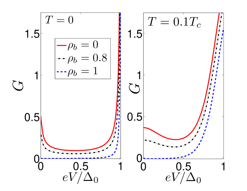
Figure 4: The voltage dependence of the normalized conductance $G$, for a N/I_sf/S_M junction, calculated from Eqs.(LABEL:Y(V)Sp,34). We set $\kappa_{T}\sqrt{D/\Delta_{0}}=0.25$ and $T=0$ in the left panel and $T/T_{c}=0.1$ in the right one. By calculating the curves we have added a small $\gamma=0.01\Delta_{0}$ as damping factor.

In Fig.(4) we plot the voltage dependence of the normalized differential conductance taking into account the contribution of the quasiparticle and subgap currents given in Eq.(LABEL:Y(V)Sp) and Eq.(34) respectively.

V Conclusions

We have studied the transport properties of a generic $X_{l}/I_{sf}/X_{r}$ junction with a spin-filter tunneling barrier $I_{sf}$. The electrodes $X_{l,r}$ can be a normal metal, a ferromagnet, or a superconductor with or without a build-in exchange field. We have derived a general expression for the tunneling conductance, Eq. (15), which is valid for arbitrary value of the exchange fields and the angles between the magnetizations. This expression generalizes the well known results for normal multilayer systems with collinear magnetization and shows how the conductance depends on the mutual orientation of the magnetization of the electrodes and the magnetic barrier, the spin-filter parameter and the spin-dependent density of the states in the normal and superconducting electrodes. We also have derived new boundary conditions for the quasiclassical Green’s functions taking into account the spin-filter effect. By using these boundary conditions we have studied the proximity effect in $N/I_{sf}/S$ system and showed that spin-filtering suppresses the amplitude of the condensate in the normal layer. In particular we show that the sub gap conductance of the $N/I_{sf}/S$ junction is suppressed due to the spin-filter effect by a factor $\sqrt{1-P_{b}^{2}}$, where $P_{b}$ is the spin-filter efficiency parameter.

References

- (1) L.N. Bulaevskii, V.V. Kuzii, and A.A. Sobyanin, JETP Lett. 25, 290 (1977).
- (2) A.I. Buzdin, L.N. Bulaevskii, and S.V. Panyukov, JETP Lett. 35, 178 (1982).
- (3) V.V. Ryazanov, V.A. Oboznov, A.Yu. Rusanov, A.V. Veretennikov, A.A. Golubov, and J. Aarts, Phys. Rev. Lett. 86, 2427 (2001); V.A. Oboznov, V.V. Bolginov, A.K. Feofanov, V.V. Ryazanov, and A.I. Buzdin, ibid 96, 197003 (2006).
- (4) T. Kontos, M. Aprili, J. Lesueur, F. Genet, B. Stephanidis, and R. Boursier, Phys. Rev. Lett. 89, 137007 (2002).
- (5) Y. Blum, A. Tsukernik, M. Karpovski, and A. Palevski, Phys. Rev. Lett. 89, 187004 (2002).
- (6) A. Bauer, J. Bentner, M. Aprili, M.L. Della-Rocca, M. Reinwald, W. Wegscheider, and C. Strunk, Phys. Rev. Lett. 92, 217001 (2004).
- (7) H. Sellier, C. Baraduc, F. Lefloch, R. Calemczuk, Phys. Rev. Lett. 92, 257005 (2004).
- (8) V. Shelukhin, A. Tsukernik, M. Karpovski, Y. Blum, K. B. Efetov, A.F. Volkov, T. Champel, M. Eschrig, T. Lofwander, G. Schon, A. Palevski, Phys. Rev. B 73,174506 (2006).
- (9) A. A. Bannykh, J. Pfeiffer, V. S. Stolyarov, I. E. Batov, V. V. Ryazanov, M. Weides, Phys. Rev. B 79, 054501 (2009).
- (10) F.S. Bergeret, A.F. Volkov, K.B. Efetov, Phys. Rev.Lett. 86, 4096 (2001).
- (11) R. S. Keizer, S. T. B. Goennenwein, T. M. Klapwijk, G. Miao, G. Xiao, A. Gupta, Nature 439, 825 (2006).
- (12) I. Sosnin, H. Cho, V. T. Petrashov, and A. F. Volkov, Phys. Rev. Lett. 96, 157002 (2006).
- (13) T. S. Khaire, M. A. Khasawneh, W. P. Pratt, Jr., N. O. Birge, Phys. Rev. Lett. 104, 137002 (2010); Carolin Klose et al., ibid 108, 127002 (2012).
- (14) M. S. Anwar, F. Czeschka, M. Hesselberth, M. Porcu, J. Aarts, Phys. Rev. B 82, 100501 (2010).
- (15) D. Sprungmann, K. Westerholt, H. Zabel, M. Weides, H. Kohlstedt, Phys. Rev. B 82, 060505 (2010).
- (16) J. W. A. Robinson, J.D.S. Witt, M. G. Blamire, Science 329, 59 (2010).
- (17) J. Wang, M. Singh, M. Tian, N. Kumar, B. Liu, C. Shi, J. K. Jain, N. Samarth, T. E. Mallouk, and M. H. W. Chan, Nature Physics 6, 389 (2010).
- (18) A. Buzdin, Rev. Mod. Phys. 77, 935 (2005).
- (19) F.S. Bergeret, A. F. Volkov, K. B. Efetov, Rev. Mod. Phys. 77, 1321 (2005).
- (20) M. Eschrig, Physics Today, 64, 43 (2011).
- (21) A.A. Golubov, M.Y. Kupriyanov, and E.Il’ichev, Rev. Mod. Phys. 76, 411 (2004).
- (22) K. B. Efetov, I. A. Garifullin, A. F. Volkov and K. Westerholt, Magnetic Heterostructures. Advances and Perspectives in Spinstructures and Spintransport. Series Springer Tracts in Modern Physics, Vol. 227. Zabel H., Bader S. D. (Eds.), (2007), P. 252; Magnetic Heterostructures. Series Springer Tracts in Modern Physics, Vol. 227. Zabel H., Farle M. (Eds.), (2012), P. 85.
- (23) X. Hao, J.S. Moodera, and R. Meservey, Phys. Rev. B 42, 8235 (1990)
- (24) T.S. Santos, J.S. Moodera, K.V. Raman, E. Negusse, J. Holroyd, J. Dvorak, M. Liberati, Y.U. Idzerda, and E. Arenholz, Phys. Rev. Lett. 101, 147201 (2008).
- (25) A. V. Zaitsev, Sov. Phys. JETP 59, 1015 (1984). .
- (26) A. Millis, D. Rainer, and J. A. Sauls, Phys. Rev. B 38, 4504 (1988).
- (27) Y. Tanaka and S. Kashiwaya, Physica C 274, 357 (1997).
- (28) M. Fogelström, Phys. Rev. B 62, 11812 (2000).
- (29) A. Cottet, D. Huertas-Hernando, W. Belzig and Yu. V. Nazarov, Phys. Rev. B 80, 184511 (2009).
- (30) M.S. Kalenkov, A. V. Galaktionov, and A. D. Zaikin, Phys. Rev. B 79, 014521 (2009).
- (31) S. Kawabata, Y. Asano, Y. Tanaka, A. A. Golubov, and S. Kashiwaya, Phys. Rev. Lett 104, 117002 (2010)
- (32) I. Zutic and O. Valls , Phys. Rev. B 61, 1555 (2000).
- (33) G.E. Blonder, M. Tinkham, and T.M. Klapwijk, Phys. Rev. B 25, 4515 (1982).
- (34) J. Linder and A. Sudbø, Phys. Rev. B 75, 134509 (2007).
- (35) J. Linder, T. Yokoyama, A. Sudbø, and M. Eschrig, Phys. Rev. Lett. 102, 107008 (2009), J. Linder, T. Yokoyama, and A. Sudbø, Phys. Rev. 79, 054523 (2009), J. Linder, A. Sudbø, T. Yokoyama, R. Grein and M. Eschrig, Phys. Rev. B 81, 214504 (2010).
- (36) F. S. Bergeret, A. Verso, and A. F. Volkov, Phys. Rev. B 86, 060506(R) (2012)
- (37) K. Senapati, M. G. Blamire, and Z. H. Barber, Nat. Mater. 10, 1 (2011).
- (38) M. Yu. Kupriyanov and V. F. Lukichev, JETP 67, 1163 (1988).
- (39) J.R. Schrieffer, Superconductivity (Benjamin, New York,(1964)).
- (40) I.O. Kulik and I.K. Yanson, Josephson effects in superconducting tunnel structures, Keter Press, Jerusalem (1972).
- (41) A.Barone and G.Paterno, Physics and applications of the Josephson effect, Wiley, NY (1982).
- (42) E. L. Wolf, Principles of electron tunneling spectroscopyxford, (University Press, Oxford,1985)
- (43) A. F. Volkov, Sov. Phys. JETP 41, 376 (1975).
- (44) S.N. Artemenko and A. F. Volkov, Zh. Eksp. Teor’ Fiz. 37, 310 (1983).
- (45) A. Moor, A. F. Volkov, K. B. Efetov, Phys. Rev. B 85, 014523 (2012).
- (46) F. S. Bergeret, A. Levy Yeyati, and A. Martín-Rodero, Phys. Rev. B 72, 064524 (2005).
- (47) F.S. Bergeret, A.F. Volkov, K.B. Efetov, Phys. Rev.Lett. 86, 3140(2001).
- (48) T. Tokuyasu, J. A. Sauls, and D. Rainer, Phys. Rev. B 38, 8823 (1988).
- (49) C. W. J. Beenakker, Phys. Rev. B 46, 12841 (1992).
- (50) A. F. Volkov, A. V. Zaitsev and T. M. Klapwijk, Physica C 203, 219 (1993).
- (51) A. Ozaeta, A. S. Vasenko, F. W. J. Hekking, and F. S. Bergeret, Phys. Rev. B 86, 060509 (2012).
- (52) A. Kastalsky, A. W. Kleinsasser, L. H. Greene, R. Bhat, F. P. Milliken, and J. P. Harbison, Phys. Rev. Lett. 67, 3026 (1991).
- (53) D. Quirion, C. Hoffmann, F. Lefloch, and M. Sanquer, Phys. Rev. B 65, 100508(R) (2002).
- (54) C. J. Lambert, R. Raimondi, V. Sweeney, and A. F. Volkov, Phys. Rev. B 55, 6015 (1997).
- (55) A. L. Shelankov, Sov. Phys. Solid State 26, 981 (1984)
- (56) M. Eschrig, Phys. Rev. B 61, 9061 (2000); ibid 80, 134511 (2009).
- (57) A. F. Volkov, JETP Lett. 55, 746 (1992); Phys. Lett. A 174, 144 (1993).
- (58) B. J. van Wees, P. de Vries, P. Magnée, and T. M. Klapwijk, Phys. Rev. Lett. 69, 510 (1992).
- (59) F. W. J. Hekking and Y. V. Nazarov, Phys. Rev. B 49, 6847 (1994).
- (60) A. V. Burmistrova and I. A. Devyatov, PisÕma v ZETF 96, 430 (2012).
- (61) A. V. Burmistrova, I. A. Devyatov, Alexander A. Golubov, Keiji Yada, Yukio Tanaka, arXiv:1210.1479
- (62) M. Julliere, Phys. Lett. 54A. 225 (1975).
- (63) J. C. Slonczewski, Phys. Rev. B 39, 6995 (1989).