DESY 12-187
SFB/CPP-12-81

A one-loop study of matching conditions for static-light flavor currents

Dirk Hesse^a,b and Rainer Sommer^a
a NIC, DESY, Platanenallee 6, 15738 Zeuthen, Germany ^b Università degli studi di Parma,

Viale G.P. Usberti n. 7/A (Parco Area delle Scienze), 43124 Parma, Italy

Abstract

Heavy Quark Effective Theory (HQET) computations of semi-leptonic decays, e.g. $B\to\pi l\nu$, require the knowledge of the parameters in the effective theory for all components of the heavy-light flavor currents. So far non-perturbative matching conditions have been employed only for the time component of the axial current. Here we perform a check of matching conditions for the time component of the vector current and the spatial component of the axial vector current up to one-loop order of perturbation theory and to lowest order of the $1/m$-expansion. We find that the proposed observables have small higher order terms in the $1/m$-series and are thus excellent candidates for a non-perturbative matching procedure.

Key words: Heavy Quark Effective Theory; Lattice QCD; Non-perturbative renormalization; Matching

PACS: 12.38.Bx; 12.38.Gc; 12.39.Hg; 13.20.He

1 Introduction

B meson decays are an excellent source of information for constraining physics beyond the Standard Model. Precision based on a solid theory and advanced experiments is becoming increasingly important as we know that effects due to fields which are not present in the Standard Model are small. Next to leptonic decays, exclusive semileptonic decays are easiest to treat in theory. Take for example the decay $B\to\pi l\nu$ which is relevant for a determination of $V_{\rm ub}$. Theory only needs to predict two form factors (in practice a single one dominates) from non-perturbative QCD. This is a strong motivation to extend the HQET programme of the ALPHA-collaboration[?,?,?,?,?,?] to include matrix elements of all components of the weak heavy-light currents. And it is a significant step beyond what has been achieved so far, where only the HQET action and the time-component of the axial current were determined non-perturbatively[?,?].

Instead of the previous five we now need 19 parameters in order to have the effective theory defined non-perturbatively including all $1/m$ terms, namely all terms of mass dimension five in the action and dimension four in the currents. Therefore, 19 matching conditions are needed. It is important to choose them well. Each matching condition simply consists of a matching observable $\Phi_{i}$ which is evaluated in QCD and in HQET — in the latter theory including the terms of order $1/m$ and no more. Setting $\Phi^{\rm QCD}_{i}=\Phi^{\rm HQET}_{i}$ determines (in fact defines) the parameters in HQET. What does it mean to choose the matching observables well? Ideally we would like each one of them to be sensitive to a single parameter in HQET, in practice we would like them to receive little contributions from terms of order $1/m^{2}$ in the effective theory. If such contributions from ${\rm O}(1/m^{2})$ terms are unnaturally large, they affect the determined parameters and then inflict unnaturally large $1/m^{2}$ terms into the observables that one wants to determine from HQET after the matching has been carried out. One thus better chooses the matching observables in QCD which are strongly dominated by the terms of order $m^{0}$ and $m^{-1}$. Since the ALPHA strategy consists of matching in a finite volume with Schrödinger functional boundary conditions, the size of different terms in the expansion is given in terms of $z^{-n}=(Lm)^{-n}$ with $L$ the linear extent of the finite volume.

Of course, in the whole process, the most important terms are those which appear at order $m^{0}$, the static terms. They are simply dominating numerically. It is thus of importance to make sure that those matching observables which determine the normalization of the static currents are chosen well. Due to the breaking of relativistic invariance we need to normalize the space and time components of the currents separately. Thus we consider the axial vector current $A_{0},A_{k}$ and the vector one $V_{0},V_{k}$. Previously, the normalization factor $Z_{\rm A_{0}}^{\rm HQET}$ of $A_{0}$ has been studied in detail [?,?,?,?,?,?,?]. It is defined through a Schrödinger functional two-point function [?]. Since in static approximation $A_{0}$ and $V_{k}$ are related through the spin symmetry (see Sect. 2 for a more precise statement), the natural condition for $Z_{\rm V_{k}}^{\rm HQET}$ follows from a simple spin rotation. However, $Z_{\rm A_{k}}^{\rm HQET}$ and $Z_{\rm V_{0}}^{\rm HQET}$ do not appear in the Schrödinger functional two-point functions which have been considered so far. We are thus lead to either consider two-point functions with more complicated kinematics or three-point functions.

In fact three-point functions appear naturally, since they are also used to determine the desired form factor for $B\to\pi l\nu$[?,?,?,?,?,?,?]. One thus uses a process in the finite volume matching which is related to one of the desired infinite volume matrix elements and there is even a potential that higher order in $1/m$ terms cancel between the matching and the physical matrix element. On the other hand, these functions have not been considered before. We therefore evaluate them first in perturbation theory, including the one-loop parts. We can then verify that they are indeed dominated by the first two terms in the $1/m$-expansion.

The perturbative study is rather straight forward, since one of us has developed “pastor”, a tool to carry out one-loop computations of Schrödinger functional correlation functions in a largely automatic manner. Still, the scope of this paper is not to consider the full system of 19 unknowns, but to study the two numerically dominating matching conditions for $Z_{\rm V_{0}}^{\rm HQET}$ and $Z_{\rm A_{k}}^{\rm HQET}$. The pastor software package was first introduced in [?] and the publication of a more thorough description along with the source code is planned for the near future.

2 The large mass limit of QCD: Heavy Quark Effective Theory

We consider QCD with at least three flavors, one of them massive, $m_{\rm b}=m$, and the others massless, in particular $m_{\rm u}=m_{\rm d}=0$. A pseudo-scalar state with the flavor content ${\rm b}\bar{\rm d}$ is written $|P_{{\rm b}\bar{\rm d}}\,,\;L\rangle$, with $L$ denoting a single external (kinematical) length scale. Analogously a light pseudo-scalar state is $|P_{{\rm u}\bar{\rm d}}\,,\;L\rangle$ and vector states are labelled with $V$ instead of $P$. We are interested in matrix elements

$$\mathcal{M}^{\mathrm{QCD}}(L,\kern 1.0pt\overline{\kern-1.0ptm\kern-1.0pt}\kern 1.0pt)=\langle X_{{\rm u}\bar{\rm d}},L|\hat{J}_{\nu}^{{\rm u}{\rm b}}({\it\bf x})|X_{{\rm b}\bar{\rm d}},L\rangle\,,\quad$$ (2.1)

of the QCD heavy-light current operators which correspond to the classical field

$$J_{\nu}^{{\rm u}{\rm b}}(x)=Z_{J}\,\overline{\psi}_{\rm u}(x)\Gamma_{\nu}\psi_{\rm b}(x)\,.$$ (2.2)

In particular we consider the axial vector current, $J_{\nu}=A_{\nu}$, with $\Gamma_{\nu}=\gamma_{5}\gamma_{\nu}$ and the vector current, $J_{\nu}=V_{\nu}$ with $\Gamma_{\nu}=\gamma_{\nu}$. In physical processes, $L$ is an inverse momentum scale, but we will later use states in a finite periodic $L\times L\times L$ volume. For the moment the relevant point is that $L$ is the only scale apart from $m$. Then there is a perturbative expansion

$$\mathcal{M}^{\mathrm{QCD}}(L,\kern 1.0pt\overline{\kern-1.0ptm\kern-1.0pt}\kern 1.0pt)=({\mathcal{M}^{\mathrm{QCD}}})^{(0)}(z)+\bar{g}^{2}(L)({\mathcal{M}^{\mathrm{QCD}}})^{(1)}(z)+{\rm O}(\bar{g}^{4}(L))\,,\quad z=L\kern 1.0pt\overline{\kern-1.0ptm\kern-1.0pt}\kern 1.0pt\,.$$ (2.3)

We will specify the renormalization scheme for $\bar{g},\kern 1.0pt\overline{\kern-1.0ptm\kern-1.0pt}\kern 1.0pt$ when it becomes relevant. The renormalization factors $Z_{J}$ of the flavor currents are to be chosen such that the currents satisfy the chiral Ward identities[?,?]. In the large mass limit, $\kern 1.0pt\overline{\kern-1.0ptm\kern-1.0pt}\kern 1.0pt\to\infty$, $L$ fixed, the matrix elements $\mathcal{M}^{\mathrm{QCD}}$ are logarithmically divergent [?,?],

$$({\mathcal{M}^{\mathrm{QCD}}})^{(1)}(z)\raisebox{-0.43057pt}{ $\stackrel{{\scriptstyle\small{z\to\infty}}}{{\sim}}$}\;H^{(1)}-\gamma_{0}\log(z)H^{(0)}\,,\quad\gamma_{0}=-1/(4\pi^{2})\,,\quad z=L\kern 1.0pt\overline{\kern-1.0ptm\kern-1.0pt}\kern 1.0pt\,.$$ (2.4)

This limit of QCD is described by an effective field theory, HQET. Up to corrections of order $1/z$, it is the static effective theory [?] where the b-field is replaced by a two-component static field,

$$\psi_{\rm b}(x)\to\psi_{\rm h}(x)=\hbox{$1\over 2$}(1+\gamma_{0})\psi_{\rm h}(x)\,,$$ (2.5)

with Lagrangian,

$${\mathscr{L}}_{\rm stat}(x)=\overline{\psi}_{\rm h}(x)(\delta m+D_{0})\psi_{\rm h}(x)\,.$$ (2.6)

The mass counter term $\delta m$ does not play a role in the following. The static flavor currents are form-identical with the QCD ones, for example $V^{\rm stat}_{0}(x)=\overline{\psi}_{\rm u}(x)\gamma_{0}\psi_{\rm h}(x)$, $A^{\rm stat}_{k}(x)=\overline{\psi}_{\rm u}(x)\gamma_{5}\gamma_{k}\psi_{\rm h}(x)$. Chiral Ward identities fix the relative normalization of the static vector and axial vector currents but not the overall normalization. Furthermore space and time-components are to be treated separately and the currents have an anomalous dimension in the effective theory. Choosing the lattice regularization we can in a first step define finite currents by renormalizing them in the lattice minimal subtraction scheme. The renormalized currents are then

$$(J_{\mathrm{lat}}^{\mathrm{stat}})_{\nu}(x;\mu)=Z_{\mathrm{lat}}(\mu a,g_{0})\,J^{\mathrm{stat}}_{\nu}(x)=Z_{\mathrm{lat}}(\mu a,g_{0})\,\overline{\psi}_{\rm u}(x)\Gamma_{\nu}\psi_{\rm h}(x)\,,$$ (2.7)

with a renormalization constant

$$Z_{\mathrm{lat}}(\mu a,g_{0})=1-\gamma_{0}\log(a\mu)g_{0}^{2}+{\rm O}(g_{0}^{4})\,,$$ (2.8)

which is common to all currents (see [?] for a pedagogical introduction). Their matrix elements

$$\mathcal{M}^{\mathrm{stat}}_{J_{\nu}}(L,\mu)=Z_{\mathrm{lat}}(\mu a,g_{0})\langle X_{{\rm u}\bar{\rm d}}|\hat{J}^{\mathrm{stat}}_{\nu}({\it\bf x})|X_{{\rm b}\bar{\rm d}}\rangle_{\mathrm{stat}}\,,$$ (2.9)

are then finite. When we set $\mu=\kern 1.0pt\overline{\kern-1.0ptm\kern-1.0pt}\kern 1.0pt$, they are equal to the corresponding QCD matrix elements up to higher order terms in $1/m$,

$$\mathcal{M}^{\mathrm{QCD}}_{J_{\nu}}(L,\kern 1.0pt\overline{\kern-1.0ptm\kern-1.0pt}\kern 1.0pt)=C_{J_{\nu}}^{\mathrm{match}}(\bar{g}^{2}(\kern 1.0pt\overline{\kern-1.0ptm\kern-1.0pt}\kern 1.0pt))\,\mathcal{M}^{\mathrm{stat}}_{J_{\nu}}(L,\kern 1.0pt\overline{\kern-1.0ptm\kern-1.0pt}\kern 1.0pt)+{\rm O}(1/\kern 1.0pt\overline{\kern-1.0ptm\kern-1.0pt}\kern 1.0pt)\,,$$ (2.10)

and up to the finite renormalization factor

$$C_{J_{\nu}}^{\mathrm{match}}(g^{2})=1+B_{J_{\nu}}g^{2}+{\rm O}(g^{4})\,.$$ (2.11)

The one-loop coefficients are

$$B_{A_{0}} = -0.137(1)\,,$$ (2.12)

$$B_{V_{0}}-B_{A_{0}} = 0.0521(1)=B_{V_{k}}-B_{A_{k}}\,,$$ (2.13)

$$B_{A_{k}}-B_{V_{0}} = -0.016900\,.$$ (2.14)

Here eq. (2.12), due to [?,?], and eq. (2.13), due to [?], depend on the lattice regularisation. They are given for the Eichten-Hill lattice action for the static quark, the ${\rm O}(a)$-improved Wilson action for the light quarks and the plaquette gauge action. We note that eq. (2.13) follows from requiring a chiral Ward identity. On the other hand the bare currents $V_{0}$ and $A_{k}$ are related by the spin symmetry of the static effective theory which is exact in lattice regularization. The difference, eq. (2.14), is therefore known very precisely from continuum perturbation theory [?]. Of course the renormalization of the fields and therefore in particular $B_{J_{\nu}}$ are independent of the states in eq. (2.1).

3 Matching conditions

3.1 Definitions of correlation functions

As discussed in the introduction, in the ALPHA strategy we use finite volume matrix elements to define the matching of HQET and QCD. These matrix elements are constructed in the Schrödinger functional, where they are exactly related to ratios of correlation functions, see [?] for more details. Here we define those correlation functions and ratios which are suitable for the matching of $V_{0}$ and $A_{k}$.

We choose the Schrödinger functional with vanishing background field, denote the time-extent by $T$ and the space-extent by $L$. As a shorthand we introduce (non-local) boundary fields

$${\cal O}_{ij}(\Gamma) = {a^{6}\over L^{3}}\sum_{{\it\bf x},{\it\bf y}}\overline{\zeta}_{i}({\it\bf x})\Gamma\zeta_{j}({\it\bf y})\,,\quad{\cal O}^{\prime}_{ij}(\Gamma)={a^{6}\over L^{3}}\sum_{{\it\bf x},{\it\bf y}}\overline{\zeta}\kern 1.0pt^{\prime}_{i}({\it\bf x})\Gamma\zeta^{\prime}_{j}({\it\bf y})\,,$$ (3.15)

where the first one creates a meson with flavor content $i\bar{j}$ at time zero and the second annihilates a meson with flavor content $j\bar{i}$ at final time $T$. The boundary quark fields $\zeta_{i},\overline{\zeta}_{i}$ are defined in [?]. For simplicity and because more sophisticated choices seem unnecessary, we take each flavor to have the same periodicity phase $\theta$ in the boundary conditions $\psi(x=L\hat{k})={\rm e}^{i\theta}\psi(x)\,,\;\overline{\psi}(x=L\hat{k})={\rm e}^{-i\theta}\overline{\psi}(x)$ .

With these preliminaries we define boundary-to-boundary correlation functions (remember $z=\kern 1.0pt\overline{\kern-1.0ptm\kern-1.0pt}\kern 1.0ptL$)

$$F_{1}^{{\rm b}{\rm d}}(\theta,z) = -\hbox{$1\over 2$}\langle{\cal O}^{\prime}_{{\rm d}{\rm b}}(\gamma_{5}){\cal O}_{{\rm b}{\rm d}}(\gamma_{5})\rangle\,,$$ (3.16)

$$F_{1}^{{\rm u}{\rm d}}(\theta) = -\hbox{$1\over 2$}\langle{\cal O}^{\prime}_{{\rm d}{\rm u}}(\gamma_{5}){\cal O}_{{\rm u}{\rm d}}(\gamma_{5})\rangle\,,$$ (3.17)

$$K_{1}^{{\rm u}{\rm d}}(\theta) = -\hbox{$1\over 2$}\langle{\cal O}^{\prime}_{{\rm d}{\rm u}}(\gamma_{k}){\cal O}_{{\rm u}{\rm d}}(\gamma_{k})\rangle\,,$$ (3.18)

and three-point correlation functions with the desired currents

$$F_{\rm V_{0}}(x_{0};\theta,z) = -\hbox{$L^{3}\over 2$}\langle{\cal O}^{\prime}_{{\rm d}{\rm u}}(\gamma_{5})V_{0}^{\rm ub}(x){\cal O}_{{\rm b}{\rm d}}(\gamma_{5})\rangle\,,$$ (3.19)

$$J^{1}_{\rm A_{1}}(x_{0};\theta,z) = -\hbox{$L^{3}\over 2$}\langle{\cal O}^{\prime}_{{\rm d}{\rm u}}(\gamma_{1})A_{1}^{\rm ub}(x){\cal O}_{{\rm b}{\rm d}}(\gamma_{5})\rangle\,.$$ (3.20)

3.2 Possible matching observables for $V_{0},A_{k}$

The defined correlation functions are easily combined to form the desired finite volume matrix elements,

$$L^{3}\mathcal{M}^{\mathrm{QCD}}_{\rm V_{0}}(L,\kern 1.0pt\overline{\kern-1.0ptm\kern-1.0pt}\kern 1.0pt) = -Z_{\rm V}\,{{F_{\rm V_{0}}(T/2;\theta,z)\over[F_{1}^{{\rm u}{\rm d}}(\theta)F_{1}^{{\rm b}{\rm d}}(\theta,z)]^{1/2}}}\,,$$ (3.21)

$$L^{3}\mathcal{M}^{\mathrm{QCD}}_{\rm A_{k}}(L,\kern 1.0pt\overline{\kern-1.0ptm\kern-1.0pt}\kern 1.0pt) = -Z_{\rm A}\,{{J^{1}_{\rm A_{1}}(T/2;\theta,z)\over[K_{1}^{{\rm u}{\rm d}}(\theta)F_{1}^{{\rm b}{\rm d}}(\theta,z)]^{1/2}}}\,,$$ (3.22)

where we set $T=L$. As explained in [?] these ratios are equal to the matrix elements eq. (2.1) with the finite volume states such as $|P_{{\rm b}\bar{\rm d}}\,,\;L\rangle$, all normalized to unity. We here neglect ${\rm O}(a)$-improvement, but this is used in the perturbative computations in Sect. 4.

We now have good candidates for matching conditions which we write in the form

$$\Phi^{\rm QCD}_{J_{\nu}}(L,\kern 1.0pt\overline{\kern-1.0ptm\kern-1.0pt}\kern 1.0pt)=\Phi^{\mathrm{stat}}_{J_{\nu}}(L,\kern 1.0pt\overline{\kern-1.0ptm\kern-1.0pt}\kern 1.0pt)+\log\left\{C_{J_{\nu}}^{\mathrm{match}}\left(\bar{g}^{2}(\kern 1.0pt\overline{\kern-1.0ptm\kern-1.0pt}\kern 1.0pt)\right)\right\}+{\rm O}(1/\kern 1.0pt\overline{\kern-1.0ptm\kern-1.0pt}\kern 1.0pt)\,,$$ (3.23)

with $\Phi^{\rm QCD}_{J_{\nu}}\equiv\log\left(L^{3}\mathcal{M}^{\mathrm{QCD}}_{J_{\nu}}\right)$. In this way the $\log(C_{J_{\nu}}^{\mathrm{match}})$-term appears additively, which is advantageous once the $1/m$-terms are included [?].

3.3 Checking their quality

Expanding eq. (3.23) in the coupling we have

$$(\Phi^{\rm QCD}_{J_{\nu}})^{(0)}(z) = (\Phi^{\mathrm{stat}}_{J_{\nu}})^{(0)}+{\rm O}(1/z)\,,$$ (3.24)

$$(\Phi^{\rm QCD}_{J_{\nu}})^{(1)}(z) = (\Phi^{\mathrm{stat}}_{J_{\nu}})^{(1)}+B_{J_{\nu}}-\gamma_{0}\log(a\kern 1.0pt\overline{\kern-1.0ptm\kern-1.0pt}\kern 1.0pt)+{\rm O}(1/z)\,.$$ (3.25)

The one-loop part can be rewritten as in eq. (2.4), namely

$$G^{(1)}_{J_{\nu}}(z) \equiv (\Phi^{\rm QCD}_{J_{\nu}})^{(1)}(z)+\gamma_{0}\log(z)=H^{(1)}_{J_{\nu}}+{\rm O}(1/z)$$ (3.26)

with

$$H^{(0)}_{J_{\nu}} = (\Phi^{\mathrm{stat}}_{J_{\nu}})^{(0)}\,,$$ (3.27)

$$H^{(1)}_{J_{\nu}} = (\Phi^{\mathrm{stat}}_{J_{\nu}})^{(1)}+B_{J_{\nu}}-\gamma_{0}\log(a/L)\,,$$ (3.28)

where we subtract the logarithmic singularity in $z$ from $(\Phi^{\rm QCD}_{J_{\nu}})^{(1)}(z)$ such that $H^{(1)}_{J_{\nu}}$ represents the one-loop coefficient of the matched static matrix element at renormalization scale $1/L$. In this form the size of $1/m$ terms is directly visible as deviations of the left hand side of eq. (3.26) from $H^{(1)}_{J_{\nu}}$. We want to investigate these deviations in the following in order to ensure that eq. (3.21) and eq. (3.22) are good observables for the matching.

4 One-loop computation

All the required quantities ($F_{\mathrm{V_{0}}}$, $J_{\mathrm{A_{1}}}^{\mathrm{1}}$, $F_{\mathrm{1}}^{\mathrm{ud}}$, $K_{\mathrm{1}}^{\mathrm{ud}}$, and their static counterparts) were calculated at the one-loop level using the pastor software package for automated lattice perturbation theory calculations [?]. As input, pastor accepts a rather general class of lattice actions and observables defined in the Schrödinger functional. It will then automatically generate computer programs for the evaluation of all contributions of the observables under investigation up to one-loop order including improvement- and counter-terms. We did implement full ${\rm O}(a)$-improvement, including the terms proportional to $am_{\rm q}$ not written in eq. (3.21) and eq. (3.22).

For the quantities in QCD, we choose lattice resolutions of $L/a$ up to 40, while for the HQET counterparts lower resolutions up to $L/a=30$ are sufficient to obtain reliable continuum extrapolations, c.f. Fig. 1. To determine the continuum limits, we employ the method described in [?] using the implementation provided by pastor. We choose $\theta\in\{0,0.5,1.0\}$ and $z\in\{4,6,8,10\}$.

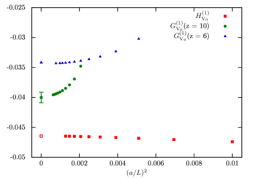
Figure 1: Continuum extrapolation of $H_{\mathrm{V_{0}}}$, $G_{\mathrm{V_{0}}}$at one-loop level, $\theta=0.5$. The round-off errors on the data points at finite $L/a$ and the uncertainty of the continuum extrapolation for the static point are much smaller than the symbol size.

We employ the mass-independent lattice minimal subtraction scheme [?] in which the ${\rm O}(a)$ improved renormalized mass at scale $\mu=1/L$ is given by

$$\overline{m}(L)=Z_{\mathrm{m},{\rm lat}}({g}_{0}^{2},a/L)\,m_{\rm q}\left[1+a\,b_{\rm m}({g}_{0}^{2})\,m_{\rm q}\right],\quad m_{\rm q}=m_{0}-m_{\rm c}\,$$ (4.29)

in terms of the bare mass of the lattice theory. At one-loop order we have [?,?]

$$b_{\rm m}({g}_{0}^{2})\; =-0.5-0.07217(2)\,C_{F}\,{g}_{0}^{2}+O({g}_{0}^{4}),$$ (4.30)

$$Z_{\mathrm{m},{\rm lat}}({g}_{0}^{2},a/L)\; =1-\hbox{$1\over 2\,\pi^{2}$}\log(a/L){g}_{0}^{2}+O({g}_{0}^{4}).$$ (4.31)

All calculations in pastor are performed with $z=\overline{m}(L)L$ as input. It inverts eq. (4.29) to obtain $m_{0}=m_{0}^{(0)}+{g}_{0}^{2}m_{0}^{(1)}+O({g}_{0}^{4})$ and calculates the series

$${\cal O}\left(m_{0}^{(0)}+{g}_{0}^{2}m_{0}^{(1)}\right)={\cal O}^{(0)}\left(m_{0}^{(0)}\right)\\ +{g}_{0}^{2}\left[{\cal O}^{(1)}\left(m_{0}^{(0)}\right)+m_{0}^{(1)}\partial_{m_{0}}{\cal O}^{(0)}\left(m_{0}^{(0)}\right)\right]+O\left({g}_{0}^{4}\right)$$ (4.32)

for a given observable ${\cal O}(m_{0})$. For the evaluation of the diagrams of a Schrödinger functional observable, it is beneficial to work in a time-momentum representation. Due to the periodic spatial boundary conditions one does not have to perform a momentum-integration but a sum over a finite set of allowed lattice momenta of size $(L/a)^{3}$. The round-off errors introduced by the numerical evaluation of this sum are estimated from the difference of long double precision and double precision results for representative parameters. Apart from this test we use double precision since it is roughly a factor three faster. The execution time to evaluate the numerically most challenging loop diagram at $L/a=40$ was about 50 hours on a single core CPU (Nehalem).

5 Results

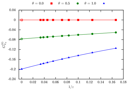
Figure 2: $G^{(0)}_{V_{0}}\equiv\left(\Phi^{\rm QCD}_{V_{0}}\right)^{(0)}(z)$ in the continuum limit. Errors are much smaller than the symbol size.

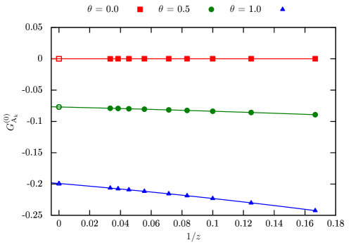
Figure 3: $G^{(0)}_{A_{1}}\equiv\left(\Phi^{\rm QCD}_{A_{1}}\right)^{(0)}(z)$ in the continuum limit. Errors are much smaller than the symbol size.

5.1 Tree-level

We start the discussion of our results with the tree-level functions $G^{(0)}_{\rm V_{0}}(z)\equiv(\Phi^{\rm QCD}_{\rm V_{0}})^{(0)}(z)$ and $G^{(0)}_{\rm A_{1}}(z)\equiv(\Phi^{\rm QCD}_{\rm A_{k}})^{(0)}(z)$. Together with the static values $H^{(0)}_{J_{\nu}}$ they are displayed in Fig. 2 and Fig. 3 for three different values of $\theta$. Curves are fits of the form $H^{(0)}(1+h_{1}/z+h_{2}/z^{2})$, fitted to the data with weights $w(z)=1/z^{3}$. The fits are thus dominated by the results at large $z$. The coefficients $h_{i}$, listed for the different cases in Table 1, are small. For all considered values of $\theta$ the $1/m$-expansion is well behaved and we can also be confident that the fitted coefficients are close to the true Taylor coefficients. Obviously, from the point of view of tree-level, one would prefer $\theta=0$ where $G^{(0)}_{J_{\nu}}(z)=H^{(0)}_{J_{\nu}}$ holds exactly.

$\theta$	0.0		0.5		1.0
	$h_{1}$	$h_{2}$	$h_{1}$	$h_{2}$	$h_{1}$	$h_{2}$
$G_{\mathrm{A_{k}}}^{(0)}$	0.00000	0.00000	0.77621	1.11933	1.05083	1.53061
$G_{\mathrm{V_{0}}}^{(0)}$	0.00000	0.00000	-2.30791	1.57043	-3.06017	3.11951
	$h_{1}$	$f_{1}$	$h_{1}$	$f_{1}$	$h_{1}$	$f_{1}$
$G_{\mathrm{A_{k}}}^{(1)}$	0.05245	-0.00132	0.12513	0.00139	0.21893	0.01547
	0.03099	0.01054	0.10547	0.01225	0.19391	0.02929
$G_{\mathrm{V_{0}}}^{(1)}$	0.15093	-0.00923	0.08803	-0.00811	0.04548	-0.01340
	0.12100	0.00692	0.07042	0.00139	0.05268	-0.01728

Table 1: Fit coefficients for $G_{\mathrm{A_{k}}}$and $G_{\mathrm{V_{0}}}$. The upper row of fit coefficients for the one-loop results comes from the fits omitting the data at $z=4$.

5.2 One-loop

We get more information at one-loop order. In order to have all finite pieces defined, we need to specify the renormalization scheme for the quark mass. As stated in Sect. 4, we take $\overline{m}$ to be the renormalized mass in the lattice minimal subtraction scheme at scale $\mu=1/L$. The continuum limit is taken as described in the previous section.

The combination $G_{J_{\nu}}^{(1)}(z)$, eq. (3.26), is shown in Fig. 4 and Fig. 5. We perform a fit to the one loop data employing a function of the form

$$G_{J_{\nu}}^{(1)}(z)=H_{J_{\nu}}^{(1)}+h_{1}/z+f_{1}\log(z)/z,$$ (5.33)

choosing in this case constant weights, as only few data point are available anyway. It is compared to a fit of the same form, omitting the data at $z=4$. The fit parameters for the one-loop quantities in Table 1 are not expected to be accurate estimates for the corresponding asymptotic expansion. The accuracy of the fits and the smallness of the coefficient $f_{1}$, however, may be taken as an indication that higher order terms in the $1/z$-expansion are not very important for the considered range in $z$.

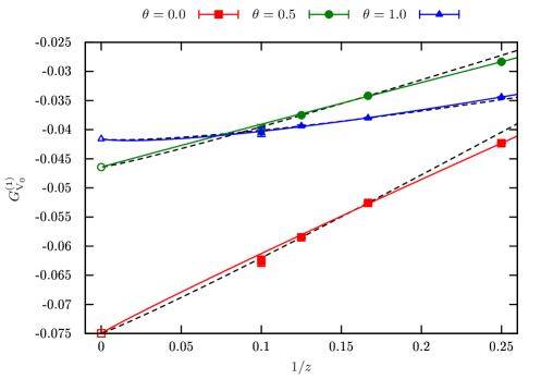
Figure 4: $G^{(1)}_{\rm V_{0}}(z)$ in the continuum limit, compared to the static result.

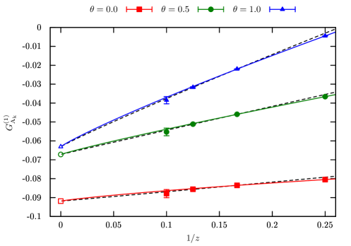
Figure 5: $G^{(1)}_{\rm A_{1}}(z)$ in the continuum limit, compared to the static result.

The size of $H^{(1)}$ is relevant for us only as a consistency check: for all cases it is a little smaller than the expected magnitude $1/(4\pi)$ for a perturbatively accessible quantity. The interesting question is the magnitude of $1/z$-terms as well as curvature when $G_{J_{\nu}}$ are considered a function of $1/z$.

We observe that also at one-loop order the $1/z$-terms in $\Phi_{J_{\nu}}$ remain small, but $\theta=0$ is not preferred any more. A choice $\theta=0.5$ appears a good compromise between tree-level and one-loop. Take for illustration $\bar{g}^{2}=4$ and $z\geq 10$ as it is typical in the non-perturbative application [?]. Then we roughly have a few per-mille $1/z$ correction at tree-level and an $\approx 3\%$ correction at one-loop. This is very acceptable. We then have all rights to expect that the $1/z^{2}$ corrections, which are omitted when HQET is treated non-perturbatively [?,?], are negligible and indeed the curvatures seen in Fig. 4 and Fig. 5 are small.

6 Conclusions

The proposed three-point functions appear very useful. They are seen to be strongly dominated by the lowest terms in the $1/z$ expansion. As a consequence, the three-point functions may well be applied to fix the remaining two unknowns, $Z_{\rm V_{0}}^{\rm HQET}$ and $Z_{\rm A_{k}}^{\rm HQET}$, in the static approximation non-perturbatively. We would recommend $\theta=0.5$, but the one-loop study does not suggest this choice to be much superior to $\theta=0$ or $\theta=1$. At order $1/m$ the full system determining the 19 parameters has to be considered. Three of these parameters come from the HQET action [?], two from the temporal components of the vector and axial vector current respectively and the spatial components of the currents require the inclusion of further six parameters each [?,?,?]. A study of this system in perturbation theory is presently being carried out by the ALPHA collaboration.

We can also confirm that the new package pastor is very useful in studying such problems in perturbation theory. This goes beyond issues related to the regularization such as renormalization factors or improvement coefficients. In fact, all results presented here refer to the $z$-dependence in continuum perturbation theory, since we were able to reliably take the continuum limit $a/L\to 0$. We have presented the results in the lattice minimal subtraction scheme for the quark mass. They can trivially be connected to the ${\rm\overline{MS\kern-0.50003pt}\kern 0.50003pt}$ scheme by using [?] $\overline{m}(L)=(1+0.122282\,\bar{g}^{2})\times\overline{m}_{\rm\overline{MS\kern-0.35002pt}\kern 0.35002pt}(1/L)+{\rm O}(\bar{g}^{4})$.
Acknowledgements. We want to thank Piotr Korcyl, Michele della Morte and Hubert Simma for helpful discussions, Jochen Heitger for a critical reading of our draft and the computing center at DESY Zeuthen for support and CPU time on the PC farm. This work has been partly funded by the Research Executive Agency (REA) of the European Union under Grant Agreement number PITN-GA-2009-238353 (ITN STRONGnet) and by the SFB/TR 9 of the Deutsche Forschungsgemeinschaft.

References

- [1] ALPHA Collaboration, J. Heitger and R. Sommer, Non-perturbative heavy quark effective theory, JHEP 02 (2004) 022, [hep-lat/0310035].
- [2] B. Blossier, M. della Morte, N. Garron, and R. Sommer, HQET at order : I. Non-perturbative parameters in the quenched approximation, JHEP 1006 (2010) 002, [arXiv:1001.4783].
- [3] ALPHA Collaboration, B. Blossier et al., HQET at order : II. Spectroscopy in the quenched approximation, JHEP 1005 (2010) 074, [arXiv:1004.2661].
- [4] ALPHA Collaboration, B. Blossier et al., HQET at order 1/m: III. Decay constants in the quenched approximation, JHEP 1012 (2010) 039, [arXiv:1006.5816].
- [5] M. Della Morte, P. Fritzsch, and J. Heitger, Non-perturbative renormalization of the static axial current in two-flavour QCD, JHEP 02 (2007) 079, [hep-lat/0611036].
- [6] B. Blossier, M. Della Morte, P. Fritzsch, N. Garron, J. Heitger, et al., Parameters of Heavy Quark Effective Theory from lattice QCD, JHEP 1209 (2012) 132, [arXiv:1203.6516].
- [7] ALPHA Collaboration, M. Kurth and R. Sommer, Renormalization and O()-improvement of the static axial current, Nucl. Phys. B597 (2001) 488–518, [hep-lat/0007002].
- [8] ALPHA Collaboration, M. Kurth and R. Sommer, Heavy quark effective theory at one-loop order: An explicit example, Nucl. Phys. B623 (2002) 271–286, [hep-lat/0108018].
- [9] J. Heitger, M. Kurth, and R. Sommer, Non-perturbative renormalization of the static axial current in quenched QCD, Nucl. Phys. B669, (2003) 173 hep-lat/0302019.
- [10] J. A. Bailey, C. Bernard, C. E. DeTar, M. Di Pierro, A. El-Khadra, et al., The semileptonic form factor from three-flavor lattice QCD: A Model-independent determination of , Phys.Rev. D79 (2009) 054507, [arXiv:0811.3640].
- [11] E. Dalgic, A. Gray, M. Wingate, C. T. Davies, G. P. Lepage, et al., B meson semileptonic form-factors from unquenched lattice QCD, Phys.Rev. D73 (2006) 074502, [hep-lat/0601021].
- [12] Z. Liu, S. Meinel, A. Hart, R. R. Horgan, E. H. Muller, et al., A Lattice calculation of form factors, arXiv:1101.2726.
- [13] ALPHA Collaboration, F. Bahr, F. Bernardoni, B. Blossier, J. Bulava, M. Della Morte, et al., determination in lattice QCD, arXiv:1211.6327.
- [14] R. Zhou, S. Gottlieb, J. A. Bailey, D. Du, A. X. El-Khadra, et al., Form factors for semi-leptonic B decays, PoS LATTICE2012 (2012) 120, [arXiv:1211.1390].
- [15] C. Bouchard, G. P. Lepage, C. J. Monahan, H. Na, and J. Shigemitsu, Form factors for and semileptonic decays with NRQCD/HISQ quarks, PoS LATTICE2012 (2012) 118, [arXiv:1210.6992].
- [16] T. Kawanai, R. S. Van de Water, and O. Witzel, The form factor from unquenched lattice QCD with domain-wall light quarks and relativistic b-quarks, PoS LATTICE2012 (2012) 109, [arXiv:1211.0956].
- [17] D. Hesse, R. Sommer, and G. von Hippel, Automated lattice perturbation theory applied to HQET, PoS LATTICE2011 (2011) 229.
- [18] L. Maiani and G. Martinelli, Current Algebra and Quark Masses from a Monte Carlo Simulation with Wilson Fermions, Phys.Lett. B178 (1986) 265.
- [19] M. Lüscher, S. Sint, R. Sommer, and H. Wittig, Nonperturbative determination of the axial current normalization constant in O() improved lattice QCD, Nucl. Phys. B491 (1997) 344–364, [hep-lat/9611015].
- [20] M. A. Shifman and M. B. Voloshin, On annihilation of mesons built from heavy and light quark and anti- oscillations, Sov. J. Nucl. Phys. 45 (1987) 292.
- [21] H. D. Politzer and M. B. Wise, Leading Logarithms of Heavy Quark Masses in Processes with Light and Heavy Quarks, Phys. Lett. B206 (1988) 681.
- [22] E. Eichten and B. Hill, An effective field theory for the calculation of matrix elements involving heavy quarks, Phys. Lett. B234 (1990) 511.
- [23] R. Sommer, Introduction to Non-perturbative Heavy Quark Effective Theory, arXiv:1008.0710. Lectures at the Summer School on “Modern perspectives in lattice QCD”, Les Houches, August 3-28, 2009.
- [24] A. Borrelli and C. Pittori, Improved renormalization constants for b-decay and mixing, Nucl. Phys. B385 (1992) 502–524.
- [25] F. Palombi, Non-perturbative renormalization of the static vector current and its O(a)-improvement in quenched QCD, JHEP 01 (2008) 021, [arXiv:0706.2460].
- [26] D. J. Broadhurst and A. G. Grozin, Matching qcd and HQET heavy-light currents at two loops and beyond, Phys. Rev. D52 (1995) 4082–4098, [hep-ph/9410240].
- [27] ALPHA Collaboration, J. Heitger, A. Juttner, R. Sommer, and J. Wennekers, Non-perturbative tests of heavy quark effective theory, JHEP 0411 (2004) 048, [hep-ph/0407227].
- [28] M. Lüscher, S. Sint, R. Sommer, and P. Weisz, Chiral symmetry and O() improvement in lattice QCD, Nucl. Phys. B478 (1996) 365–400, [hep-lat/9605038].
- [29] ALPHA Collaboration, A. Bode, P. Weisz, and U. Wolff, Two loop computation of the Schrödinger functional in lattice QCD, Nucl. Phys. B576 (2000) 517–539, [hep-lat/9911018]. Erratum-ibid.B600:453,2001, Erratum-ibid.B608:481,2001.
- [30] S. Sint and P. Weisz, Further results on o() improved lattice QCD to one loop order of perturbation theory, Nucl. Phys. B502 (1997) 251, [hep-lat/9704001].
- [31] E. Gabrielli, G. Martinelli, C. Pittori, G. Heatlie, and C. T. Sachrajda, Renormalization of lattice two fermion operators with improved nearest neighbor action, Nucl. Phys. B362 (1991) 475–486.
- [32] B. Blossier, J. Bulava, M. Della Morte, M. Donnellan, P. Fritzsch, et al., and from non-perturbatively renormalized HQET with light quarks, PoS LATTICE2011 (2011) 280, [arXiv:1112.6175].
- [33] E. Eichten and B. Hill, Static effective field theory: 1/m corrections, Phys. Lett. B243 (1990) 427–431.
- [34] A. F. Falk and B. Grinstein, Power corrections to leading logs and their application to heavy quark decays, Phys.Lett. B247 (1990) 406–411.
- [35] A. F. Falk, M. Neubert, and M. E. Luke, The Residual mass term in the heavy quark effective theory, Nucl.Phys. B388 (1992) 363–375, [hep-ph/9204229].
- [36] M. Neubert, Short distance expansion of heavy quark currents, Phys.Rev. D46 (1992) 2212–2227.