Tides in rotating barotropic fluid bodies: the contribution of inertial waves and the role of internal structure

Abstract

We discuss the linear response to low-frequency tidal forcing of fluid bodies that are slowly and uniformly rotating, are neutrally stratified and may contain a solid or fluid core. This problem may be regarded as a simplified model of astrophysical tides in convective regions of stars and giant planets. The response can be separated into non-wavelike and wavelike parts, where the former is related instantaneously to the tidal potential and the latter may involve resonances or other singularities. The imaginary part of the potential Love number of the body, which is directly related to the rates of energy and angular momentum exchange in the tidal interaction and to the rate of dissipation of energy, may have a complicated dependence on the tidal frequency. However, a certain frequency-average of this quantity is independent of the dissipative properties of the fluid and can be determined by means of an impulse calculation. The result is a strongly increasing function of the size of the core when the tidal potential is a sectoral harmonic, especially when the body is not strongly centrally condensed. However, the same is not true for tesseral harmonics, which receive a richer response and may therefore be important in determining tidal evolution even though they are usually subdominant in the expansion of the tidal potential. We also discuss analytically the low-frequency response of a slowly rotating homogeneous fluid body to tidal potentials proportional to spherical harmonics of degrees less than five. Tesseral harmonics of degrees greater than two, such as are present in the case of a spin-orbit misalignment, can resonate with inertial modes of the full sphere, leading to an enhanced tidal interaction.

1 Introduction

The tidal interaction of two bodies orbiting about their centre of mass is one of the fundamental problems of theoretical astrophysics. It is relevant to a wide variety of systems, including close binary stars, the satellites of solar-system bodies, and stars orbiting the black holes in galactic centres. Interest in this subject has grown through the discovery in recent years of numerous planets in orbits of a few days or less around other stars. It is likely that tidal interactions have affected the orbital and spin properties of many of these planets as well as providing a source of heat. Equally importantly, they may also have led to the destruction of many planets that are not observed.

Tidal theory involves a combination of celestial mechanics and continuum mechanics. The celestial mechanics is non-trivial, and has been widely investigated using highly simplistic descriptions or parametrizations of the fluid or solid behaviour (e.g. Darwin, 1880; Jeffreys, 1961; Goldreich, 1963; Goldreich & Soter, 1966; Alexander, 1973; Mignard, 1980; Hut, 1981; Eggleton, Kiseleva & Hut, 1998; Mardling & Lin, 2002; Barker & Ogilvie, 2009). In fact, the fluid dynamics of tidally forced bodies is a much richer and more difficult problem, even in a linear theory where the tide is treated as an infinitesimal disturbance. In the case of stars, the work of Zahn (1977, and references therein) identified two potentially important processes: the interaction of tidal bulges with turbulent convection and the excitation and damping of internal gravity waves in radiative zones (see also Savonije & Papaloizou, 1983; Goldreich & Nicholson, 1989; Terquem et al., 1998; Goodman & Dickson, 1998; Barker & Ogilvie, 2010). Rotation was neglected in this work in order to simplify the calculations. Its effects have been considered by Witte & Savonije (1999) and Savonije & Witte (2002) within the ‘traditional approximation’, which is usually applicable to the radiative zones of slowly rotating stars.

More recent work has examined the effects of the full Coriolis force on tides in convective zones (Ogilvie & Lin 2004; Wu 2005a, b; Papaloizou & Ivanov 2005; Ogilvie 2005; Ogilvie & Lin 2007; Goodman & Lackner 2009; Ogilvie 2009; Rieutord & Valdettaro 2010; see also Savonije, Papaloizou & Alberts 1995; Savonije & Papaloizou 1997; Papaloizou & Savonije 1997). All of these papers show that inertial waves, for which the Coriolis force provides the restoring force, can be excited by tidal forcing and may provide an important route for tidal dissipation in rotating bodies. However, even the linear theory of inertial waves is a very intricate problem and these authors come to different conclusions. In some cases the response is dominated by wave attractors, critical latitudes or other singularities, while in others global normal modes are excited. Different predictions are made for the frequency-dependence of the tidal dissipation rate. For example, while Ogilvie & Lin (2004), Ogilvie (2009) and Rieutord & Valdettaro (2010) allow inertial waves to undergo multiple reflections within a spherical shell before being damped by viscosity, and obtain a highly frequency-dependent dissipation rate, Goodman & Lackner (2009) do not allow any reflections of waves after their generation from the boundary of the planetary (or stellar) core, but instead consider nonlinear damping and obtain a smooth dissipation rate that increases with the fifth power of the core size. Nevertheless, Ogilvie (2009) found that the frequency-averaged dissipation rate with multiple reflections shows the same dependence on core size.

One purpose of this paper is to show that, in spite of this complexity, some broader aspects of the tidal response of rotating bodies are robust and insensitive to the details that distinguish between these calculations. Even if the linear theory of inertial waves in a perfect spherical shell cannot be applied reliably to the turbulent convective zone of a star or planet, the results presented here on frequency-integrated responses should still be valid.

A second purpose of this paper is to collect some analytical results on the tidal response of a homogeneous fluid body. When potential components other than the usual $l=m=2$ spherical harmonic are considered, a richer response is possible and numerous resonances can occur with large-scale inertial modes, especially in systems with a spin-orbit misalignment. Similar behaviour can be expected in more realistic models, and the astrophysical consequences require further investigation.

2 Spheroidal and toroidal vector fields

We begin with a definition that is important for the analysis in this paper. Let $(r,\theta,\phi)$ be spherical polar coordinates, and ${\mn@boldsymbol{e}}_{r}={\mn@boldsymbol{r}}/r$ the radial unit vector. A general differentiable vector field ${\mn@boldsymbol{v}}$ can be represented in the form

$${\mn@boldsymbol{v}}={\mn@boldsymbol{e}}_{r}\,R-{\mn@boldsymbol{e}}_{r}\times({\mn@boldsymbol{e}}_{r}\times{\mn@boldsymbol{\nabla}}S)-{\mn@boldsymbol{e}}_{r}\times{\mn@boldsymbol{\nabla}}T,$$ (1)

where $R$, $S$ and $T$ are scalar functions of $(r,\theta,\phi)$. Thus ${\mn@boldsymbol{v}}={\mn@boldsymbol{v}}_{\mathrm{s}}+{\mn@boldsymbol{v}}_{\mathrm{t}}$, where the spheroidal and toroidal parts of ${\mn@boldsymbol{v}}$ are

$${\mn@boldsymbol{v}}_{\mathrm{s}}={\mn@boldsymbol{e}}_{r}\,R-{\mn@boldsymbol{e}}_{r}\times({\mn@boldsymbol{e}}_{r}\times{\mn@boldsymbol{\nabla}}S),$$ (2)

$${\mn@boldsymbol{v}}_{\mathrm{t}}=-{\mn@boldsymbol{e}}_{r}\times{\mn@boldsymbol{\nabla}}T.$$ (3)

This nomenclature is used, for example, in seismology (e.g. Lapwood & Usami, 1981) and stellar oscillations (e.g. Smeyers, 2010), and is related to the theory of vector spherical harmonics (e.g. Morse & Feshbach, 1953). We have

$${\mn@boldsymbol{e}}_{r}\cdot{\mn@boldsymbol{v}}=R,$$ (4)

$${\mn@boldsymbol{e}}_{r}\cdot{\mn@boldsymbol{\nabla}}\times(-{\mn@boldsymbol{e}}_{r}\times{\mn@boldsymbol{v}})=-\nabla_{\mathrm{h}}^{2}S,$$ (5)

$${\mn@boldsymbol{e}}_{r}\cdot{\mn@boldsymbol{\nabla}}\times{\mn@boldsymbol{v}}=-\nabla_{\mathrm{h}}^{2}T,$$ (6)

where

$$\nabla_{\mathrm{h}}^{2}=\frac{1}{r^{2}\sin\theta}\frac{\partial}{\partial\theta}\left(\sin\theta\frac{\partial}{\partial\theta}\right)+\frac{1}{r^{2}\sin^{2}\theta}\frac{\partial^{2}}{\partial\phi^{2}}$$ (7)

is the horizontal part of the Laplacian operator. On each sphere $r=\mathrm{constant}>0$, the operator $\nabla_{\mathrm{h}}^{2}$ has a complete set of eigenfunctions (spherical harmonics) and can be inverted uniquely except for the addition of an arbitrary constant. Therefore, given a differentiable vector field ${\mn@boldsymbol{v}}$, equations (4)–(6) determine $R$, $S$ and $T$ uniquely except that arbitrary functions of $r$ only can be added to $S$ and $T$.

In Ogilvie & Lin (2004) and Ogilvie (2009) the velocity field is separated into spheroidal and toroidal parts and expanded in spherical harmonics. The coefficients $a_{n}$ and $b_{n}$ refer to the spheroidal part ($R$ and $S$), while the coefficients $c_{n}$ refer to the toroidal part ($T$). In Ogilvie (2009), for example, we have

$$R=\sum_{n}a_{n}(r)Y_{n}^{m}(\theta,\phi),$$ (8)

$$S=r^{2}\sum_{n}b_{n}(r)Y_{n}^{m}(\theta,\phi),$$ (9)

$$T=r^{2}\sum_{n}c_{n}(r)Y_{n}^{m}(\theta,\phi),$$ (10)

where the sums are over integers $n\geq m\geq 0$,

$$Y_{n}^{m}(\theta,\phi)=\left[\frac{(2n+1)(n-m)!}{4\pi(n+m)!}\right]^{1/2}P_{n}^{m}(\cos\theta)\,\mathrm{e}^{\mathrm{i}m\phi}$$ (11)

is a spherical harmonic with the normalization

$$\int_{0}^{2\pi}\int_{0}^{\pi}|Y_{n}^{m}(\theta,\phi)|^{2}\,\sin\theta\,\mathrm{d}\theta\,\mathrm{d}\phi=1,$$ (12)

and the real part of these expressions is to be taken after they are multiplied by $\mathrm{e}^{-\mathrm{i}\omega t}$.

3 Tidal response of a homogeneous rotating body

Perhaps the simplest tidal problem is the linear response of a homogeneous fluid sphere to a tidal potential that is harmonic in time and proportional to a solid spherical harmonic (see Thomson, 1863, although his analysis is mainly for an elastic solid rather than a fluid). To include the effects of rotation, we should properly consider an ellipsoidal figure of equilibrium (Chandrasekhar, 1969); tides in a Maclaurin spheroid were analysed by Bryan (1889), although the full ramifications of his work have not yet been explored. In the limit of slow rotation, however, it is adequate to neglect centrifugal effects and consider a spherical fluid body subject to the Coriolis force.

The tidal gravitational potential experienced by a body can be written as an interior multipole expansion in solid spherical harmonics of degrees $l\geq 2$; this series converges more rapidly when the tide-raising body is more distant. For each value of $l$, the response of a rotating body also depends on the order $m$ of the spherical harmonic, which satisfies $-l\leq m\leq l$. (The response for negative values of $m$ can be deduced from that for positive $m$ by complex conjugation if the frequency is also changed in sign.)

We collect in Appendix A some analytical results on the linear response of a homogeneous sphere to forcing by solid spherical harmonics with degrees $l=\{2,3,4\}$, i.e. interior quadrupolar, octupolar and hexadecapolar potentials. (No tidal force is generated by $l=0$ or $l=1$.) This analysis makes use of the decomposition of the tidal response into non-wavelike and wavelike parts, developed in Section 4.4 below.

In general, the tidal response involves resonances with inertial modes of the sphere when the tidal frequency matches the eigenfrequency of an appropriate inertial mode. The eigenfrequencies of inertial modes in the frame that rotates with the angular velocity $\Omega$ of the body are dense in the interval $(-2\Omega,2\Omega)$ (Greenspan, 1968). However, the selection rules determined by the spatial structure of the inertial modes and the forcing functions imply that any spherical harmonic potential resonates with only a finite number of inertial modes. Indeed, as found in Appendix A, the sectoral harmonics ($|m|=l$) do not resonate with any inertial modes, while the tesseral harmonics ($|m|<l$) do have such resonances.

However, the resonances of the quadrupolar tesseral harmonics $Y_{2}^{0}$ and $Y_{2}^{1}$ are only formal resonances and should not lead to enhanced dissipation in linear theory. The formally resonant modes have zero frequency in an inertial frame of reference; they are present because of the existence of a continuous family of equilibrium solutions for uniformly rotating bodies that have angular velocity vectors that differ in magnitude and/or direction. In the case $m=0$ the zero-frequency mode is the ‘spin-up’ mode, which consists simply of an infinitesimal uniform change in the angular velocity of the fluid. In the case $m=1$ it is the ‘spin-over’ mode of frequency $\omega=-\Omega$ (i.e. zero frequency in the inertial frame), which consists of an infinitesimal tilt of the rotation axis of the fluid. Each mode involves a change in the exactly conserved angular momentum of the body and therefore has zero frequency. The formal resonances of $Y_{2}^{0}$ and $Y_{2}^{1}$ with these modes could not produce any tidal dissipation because the modes concerned involve uniform rotation and the resonance occurs at zero forcing frequency (in the inertial frame). It may be surprising that the spin-up mode, which involves a change in the angular velocity of the fluid, can be excited by an axisymmetric tidal potential proportional to $Y_{2}^{0}$, which cannot change the axial component of angular momentum of the body. In fact, even in the absence of a torque, the spin-up mode is excited because the axisymmetric tidal deformation modulates the moment of inertia of the body.

The most important harmonic present in the tidal potential is usually considered to be $Y_{2}^{2}$, and the fact that it cannot resonantly excite inertial normal modes in a homogeneous full sphere has been noted previously (e.g. Goodman & Lackner, 2009). However, given that tesseral harmonics have a richer response in a homogeneous body, and therefore presumably also in an inhomogeneous body, other harmonics are worthy of consideration, even if they are subdominant in the expansion of the tidal potential.

To illustrate this, we consider here the case of two bodies in a circular orbit of angular velocity (or mean motion) $n$. We consider the tide raised by body 2 in body 1, which rotates uniformly, and assume that the orbit is inclined with respect to the equatorial plane of body 1. [Related analyses are given by Barker & Ogilvie (2009) and Lai (2012).] We consider four spherical polar coordinate systems, all centred on body 1:

1. aligned with the orbit, rotating with the orbit

2. aligned with the orbit, non-rotating

3. aligned with the spin of body 1, non-rotating

4. aligned with the spin of body 1, rotating with body 1

In $S_{1}$ the tide-raising body (as represented by its centre of mass) is stationary and lies in the plane $\theta=\pi/2$. The tidal potential is independent of time and can be expanded in solid spherical harmonics. Let us focus on terms of a fixed degree $l\geq 2$. Then harmonics of orders $m=\{l,\,l-2,\,l-4,\,\dots,\,-l\}$ are present, because symmetry about the plane $\theta=\pi/2$ requires that $l-m$ be even. In $S_{2}$ the tide-raising body executes a circular orbit in the plane $\theta=\pi/2$. The tidal potential involves the same spherical harmonics but their angular frequencies are now $mn$. The rotation from $S_{2}$ to $S_{3}$ mixes all permissible values of $m$ for a given $l$ (as described by the Wigner $D$-matrix). In $S_{3}$, therefore, all values of $m$ with $-l\leq m\leq l$ are present and the frequencies are $\{l,\,l-2,\,l-4,\,\dots,\,-l\}n$ for each $m$. Finally, in $S_{4}$, all values of $m$ are present and the frequencies are $\{l,\,l-2,\,l-4,\,\dots,\,-l\}n-m\Omega$, where $\Omega$ is the spin angular velocity of body 1.

In Appendix A we show that, in $S_{4}$, forcing by $Y_{3}^{m}$ resonates with an inertial mode of the sphere at frequencies

$$\omega=\frac{2}{3}\left[-m\pm\left(\frac{9-m^{2}}{5}\right)^{1/2}\right]\Omega$$ (13)

for $-2\leq m\leq 2$. Resonance with the octupolar tide therefore occurs when

$$\frac{n}{\Omega}=\pm\{0,\,0.1700,\,0.2981,\,0.3922,\,0.4444,\,0.5099,$$

$$\qquad 0.8944,\,1.1766,\,1.3333\}.$$

Similarly, forcing by $Y_{4}^{m}$ resonates with an inertial mode at frequencies that satisfy the cubic equation

$$42\left(\frac{\omega}{\Omega}\right)^{3}+63m\left(\frac{\omega}{\Omega}\right)^{2}-36(2-m^{2})\frac{\omega}{\Omega}-4m(11-2m^{2})=0$$ (15)

for $-3\leq m\leq 3$. Resonance with the hexadecapolar tide therefore occurs when

$$\frac{n}{\Omega}=\pm\{0,\,0.0970,\,0.1770,\,0.1920,\,0.1940,\,0.25,$$ (16)

$$\qquad 0.3273,\,0.3540,\,0.3840,\,0.4550,\,0.5,$$

$$\qquad 0.5580,\,0.625,\,0.6547,\,0.9100,\,1.1160,\,1.25\}.$$

It is likely that these resonances persist, albeit with modifications, in more realistic models of stars and giant planets. The resonances at smaller values of $n/\Omega$ may be expected to play a role in the tidal synchronization of close binary stars and possibly of hot Jupiters, although in the latter case tidal potential components beyond the quadrupolar ones are intrinsically very weak because of the large ratio of orbital semimajor axis to planetary radius. The resonances at larger values of $n/\Omega$, close to unity, could be important for the more rapidly rotating hosts of hot Jupiters, such as F stars, where spin-orbit misalignments are common (Albrecht et al., 2012), although the convective zones of these stars are of limited extent.

4 Tidal forcing of a rotating barotropic fluid

4.1 Equilibrium

A barotropic fluid is one in which the pressure $p$ is uniquely related to the density $\rho$. This situation arises, in particular, when the specific entropy of the fluid does not vary in space or time. The differential relations between the pressure, specific volume $v=1/\rho$, specific internal energy $e$ and specific enthalpy $h=e+pv$ are then $\mathrm{d}e=-p\,\mathrm{d}v$ and $\mathrm{d}h=v\,\mathrm{d}p$. The sound speed is $v_{\mathrm{s}}=\sqrt{\mathrm{d}p/\mathrm{d}\rho}$, so that $\mathrm{d}h=v_{\mathrm{s}}^{2}\,\mathrm{d}\rho/\rho$.

In a frame of reference that rotates with uniform angular velocity ${\mn@boldsymbol{\Omega}}$, an ideal barotropic fluid satisfies the equation of motion,

$$\frac{\partial{\mn@boldsymbol{u}}}{\partial t}+{\mn@boldsymbol{u}}\cdot{\mn@boldsymbol{\nabla}}{\mn@boldsymbol{u}}+2{\mn@boldsymbol{\Omega}}\times{\mn@boldsymbol{u}}=-{\mn@boldsymbol{\nabla}}(h+\Phi_{\mathrm{g}}+\Phi_{\mathrm{c}}),$$ (17)

and the equation of mass conservation,

$$\frac{\partial\rho}{\partial t}+{\mn@boldsymbol{\nabla}}\cdot(\rho{\mn@boldsymbol{u}})=0,$$ (18)

where ${\mn@boldsymbol{u}}$ is the velocity, $\Phi_{\mathrm{g}}$ is the gravitational potential, which satisfies Poisson’s equation,

$$\nabla^{2}\Phi_{\mathrm{g}}=4\pi G\rho,$$ (19)

and

$$\Phi_{\mathrm{c}}=-\frac{1}{2}|{\mn@boldsymbol{\Omega}}\times{\mn@boldsymbol{r}}|^{2}$$ (20)

is the centrifugal potential.

Steady axisymmetric solutions can be found in which the fluid is uniformly rotating and therefore has ${\mn@boldsymbol{u}}=\mathbf{0}$ in the appropriate frame of reference. Such solutions satisfy the equilibrium condition

$$h+\Phi_{\mathrm{g}}+\Phi_{\mathrm{c}}=\mathrm{constant}.$$ (21)

We assume that the barotropic relation is such that $p$ is an increasing function of $\rho$ for all $\rho>0$, and that $p\propto\rho^{1+1/n}$ in the limit $\rho\to 0$, where $n$ is a (finite) positive real number. In this case $\rho$ and $p$ are increasing functions of $h$ for all $h>0$, and $\rho\propto h^{n}$, $p\propto h^{n+1}$ and $v_{\mathrm{s}}^{2}\propto h$ in the limit $h\to 0$; the simplest example of such a barotropic relation is the polytrope, in which these power laws hold for all $h>0$. The body then exists where $h>0$, and can have a free surface on which $h=0$, while the normal enthalpy gradient is typically non-zero there. If $n<1$, the normal density gradient is weakly singular on the surface.

We will also consider the case of a homogeneous incompressible fluid, for which $\rho=\mathrm{constant}$. Although this case resembles the limit $n\to 0$ of the family of polytropes, it is best treated separately because the density is non-zero at the free surface.

4.2 Linearized equations

We consider a steady axisymmetric body (‘body 1’) that is weakly perturbed by a tidal gravitational potential $\Psi$, which need not be steady or axisymmetric. The tidal potential is generated by a external body (‘body 2’) and satisfies Laplace’s equation $\nabla^{2}\Psi=0$ within body 1.

The linearized equations governing the response of body 1 are

$$\ddot{\mn@boldsymbol{\xi}}+2{\mn@boldsymbol{\Omega}}\times\dot{\mn@boldsymbol{\xi}}=-{\mn@boldsymbol{\nabla}}W,$$ (22)

$$W=h^{\prime}+\Phi^{\prime}+\Psi,$$ (23)

$$\rho^{\prime}=-{\mn@boldsymbol{\nabla}}\cdot(\rho\mn@boldsymbol{\xi}),$$ (24)

$$\nabla^{2}\Phi^{\prime}=4\pi G\rho^{\prime},$$ (25)

where the prime denotes an Eulerian perturbation, the dot denotes $\partial/\partial t$, and $\mn@boldsymbol{\xi}$ is the displacement, such that ${\mn@boldsymbol{u}}^{\prime}=\dot{\mn@boldsymbol{\xi}}$. Note that $\Phi^{\prime}$ represents the internal (self-) gravitational potential perturbation, while $\Psi$ is the external (tidal) potential. Outside the fluid, $\Phi^{\prime}$ satisfies Laplace’s equation and decays to zero as $|{\mn@boldsymbol{r}}|\to\infty$. Equation (24) implies that

$$h^{\prime}=-v_{\mathrm{s}}^{2}({\mn@boldsymbol{\nabla}}\cdot\mn@boldsymbol{\xi})-\mn@boldsymbol{\xi}\cdot{\mn@boldsymbol{\nabla}}h.$$ (26)

The desired solution of these equations is such that $\mn@boldsymbol{\xi}$, ${\mn@boldsymbol{\nabla}}\cdot\mn@boldsymbol{\xi}$, $W$ and ${\mn@boldsymbol{\nabla}}W$ are bounded everywhere within the fluid, while $\Phi^{\prime}$ and ${\mn@boldsymbol{\nabla}}\Phi^{\prime}$ are bounded and continuous everywhere and tend to zero as $|{\mn@boldsymbol{r}}|\to\infty$. If $n<1$, then $\rho^{\prime}$ is weakly singular on the surface, but equation (25) still has a solution such that $\Phi^{\prime}$ and ${\mn@boldsymbol{\nabla}}\Phi^{\prime}$ are bounded and continuous.

The body may contain a solid core. Since a discussion of solid mechanics is beyond the scope of this paper, we assume that the core is perfectly rigid. The boundary condition $\mn@boldsymbol{\xi}\cdot{\mn@boldsymbol{n}}=0$ then applies on the surface of the core. However, we will also consider a fluid core in Section 4.9.

4.3 Love numbers, energy and angular momentum

From the above linearized equations and boundary conditions, after some integration by parts, we obtain an energy equation of the form

$$\frac{\mathrm{d}E}{\mathrm{d}t}=P,$$ (27)

where

$$E=\int\frac{1}{2}\rho\left(|\dot{\mn@boldsymbol{\xi}}|^{2}+\frac{h^{\prime 2}}{v_{\mathrm{s}}^{2}}\right)\,\mathrm{d}V-\frac{1}{8\pi G}\int|{\mn@boldsymbol{\nabla}}\Phi^{\prime}|^{2}\,\mathrm{d}V$$ (28)

is the (canonical) energy of the perturbation, and

$$P=\int\rho\dot{\mn@boldsymbol{\xi}}\cdot(-{\mn@boldsymbol{\nabla}}\Psi)\,\mathrm{d}V$$ (29)

is the power input by the tidal force. Integrals that involve $\rho$ are carried out over the entire fluid volume of body 1, while those that do not are carried out over all space. The energy $E$ is positive definite for a gravitationally stable body.

After an integration by parts, we have

$$P=-\int\Psi\dot{\rho}^{\prime}\,\mathrm{d}V=-\frac{1}{4\pi G}\int\Psi\nabla^{2}\dot{\Phi}^{\prime}\,\mathrm{d}V.$$ (30)

The latter integral can be carried out over any region that includes the fluid volume of body 1. Let $V_{*}$ be any such region that is simply connected and does not include body 2, so that $\nabla^{2}\Psi=0$ in $V_{*}$. Then, by Green’s second identity,

$$P = \frac{1}{4\pi G}\int_{V_{*}}(\dot{\Phi}^{\prime}\nabla^{2}\Psi-\Psi\nabla^{2}\dot{\Phi}^{\prime})\,\mathrm{d}V$$ (31)

$$= \frac{1}{4\pi G}\int_{\partial V_{*}}(\dot{\Phi}^{\prime}{\mn@boldsymbol{\nabla}}\Psi-\Psi{\mn@boldsymbol{\nabla}}\dot{\Phi}^{\prime})\cdot\mathrm{d}{\mn@boldsymbol{S}}.$$

We assume that $V_{*}$ can be chosen such that its boundary $\partial V_{*}$ is a sphere of some radius $a$ centred on body 1, i.e. that the two bodies are sufficiently distant that they can be separated by a spherical boundary. Then, in the vicinity of $\partial V_{*}$, $\Psi$ can be represented using an interior multipole expansion in solid spherical harmonics, while $\Phi^{\prime}$ can be represented using an exterior multipole expansion. Thus

$$\Psi=\sum_{l,m}\Psi_{l}^{m}(t)\left(\frac{r}{R}\right)^{l}Y_{l}^{m}(\theta,\phi),$$ (32)

$$\Phi^{\prime}=\sum_{l,m}\Phi_{l}^{m}(t)\left(\frac{r}{R}\right)^{-(l+1)}Y_{l}^{m}(\theta,\phi),$$ (33)

where $R$ is the nominal (e.g. equatorial) radius of body 1 and the sum is over integers $l\geq 2$ and $-l\leq m\leq l$. Since $\Psi$ and $\Phi^{\prime}$ are real, we have $\Psi_{l}^{-m}=\left(\Psi_{l}^{m}\right)^{*}$ and $\Phi_{l}^{-m}=\left(\Phi_{l}^{m}\right)^{*}$. Having chosen $\partial V_{*}$ to be the sphere of radius $a$, we find

$$P=\sum_{l,m}\frac{(2l+1)R}{4\pi G}\,\dot{\Phi}_{l}^{m}\left(\Psi_{l}^{m}\right)^{*},$$ (34)

which is independent of the parameter $a$, as expected.

An initial-value problem can be solved by Fourier (or Laplace) transform methods. If the tidal potential is applied for a finite time or decays sufficiently rapidly as $t\to\infty$, the total amount of energy transferred to the body is, by Parseval’s theorem,

$$\Delta E = \int_{-\infty}^{\infty}P\,\mathrm{d}t$$

$$= \sum_{l,m}\frac{(2l+1)R}{4\pi G}\int_{-\infty}^{\infty}\dot{\Phi}_{l}^{m}(t)[\Psi_{l}^{m}(t)]^{*}\,\mathrm{d}t$$

$$= \sum_{l,m}\frac{(2l+1)R}{4\pi G}\int_{-\infty}^{\infty}(-\mathrm{i}\omega)\tilde{\Phi}_{l}^{m}(\omega)[\tilde{\Psi}_{l}^{m}(\omega)]^{*}\,\frac{\mathrm{d}\omega}{2\pi},$$

where

$$\tilde{\Psi}_{l}^{m}(\omega)=\int_{-\infty}^{\infty}\Psi_{l}^{m}(t)\,\mathrm{e}^{\mathrm{i}\omega t}\,\mathrm{d}t,$$ (36)

etc., denote temporal Fourier transforms. Taking the Fourier transform of the linearized equations (22)–(25) leads to a purely spatial problem in which the frequency $\omega$ (which may in general be treated as a complex number) appears as a parameter. For a body of arbitrary shape, the solution of this problem yields a linear relation of the form

$$\tilde{\Phi}_{l}^{m}(\omega)=\sum_{l^{\prime},m^{\prime}}k_{l,l^{\prime}}^{m,m^{\prime}}(\omega)\tilde{\Psi}_{l^{\prime}}^{m^{\prime}}(\omega),$$ (37)

involving an array of potential Love numbers $k_{l,l^{\prime}}^{m,m^{\prime}}(\omega)$. The Love numbers are dimensionless complex coefficients that quantify the frequency-dependent response of the body to tidal forcing; since gravity is the only means of communication between the two bodies, all the information relevant to spin–orbit coupling and tidal evolution is contained within them. If the body is spherically symmetric then $k_{l,l^{\prime}}^{m,m^{\prime}}(\omega)=0$ unless $l^{\prime}=l$ and $m^{\prime}=m$. Let us assume instead that the body is axisymmetric (in the selected spherical polar coordinate system), so that $k_{l,l^{\prime}}^{m,m^{\prime}}(\omega)=0$ unless $m^{\prime}=m$. Since the linearized equations are invariant under complex conjugation, we also have $k_{l,l^{\prime}}^{m,m}(\omega)=[k_{l,l^{\prime}}^{-m,-m}(-\omega^{*})]^{*}$. Then

$$\Delta E=\sum_{l,m}\sum_{l^{\prime}}\frac{(2l+1)R}{4\pi G}$$ (38)

$$\times\int_{-\infty}^{\infty}(-\mathrm{i}\omega)k_{l,l^{\prime}}^{m,m}(\omega)\tilde{\Psi}_{l^{\prime}}^{m}(\omega)[\tilde{\Psi}_{l}^{m}(\omega)]^{*}\,\frac{\mathrm{d}\omega}{2\pi}.$$

Consider an idealized problem in which only a single component $\Psi_{l}^{m}$ of the tidal potential is applied. In fact, because $\Psi$ is real, $\Psi_{l}^{-m}=\left(\Psi_{l}^{m}\right)^{*}$ must also be present, and their Fourier transforms are related by $\tilde{\Psi}_{l}^{-m}(\omega)=[\tilde{\Psi}_{l}^{m}(-\omega^{*})]^{*}$. Then, if $m\neq 0$,

$$\Delta E = \frac{(2l+1)R}{4\pi G}\int_{-\infty}^{\infty}(-\mathrm{i}\omega)k_{l}^{m}(\omega)|\tilde{\Psi}_{l}^{m}(\omega)|^{2}\,\frac{\mathrm{d}\omega}{2\pi}$$ (39)

$$+\frac{(2l+1)R}{4\pi G}\int_{-\infty}^{\infty}(-\mathrm{i}\omega)k_{l}^{-m}(\omega)|\tilde{\Psi}_{l}^{-m}(\omega)|^{2}\,\frac{\mathrm{d}\omega}{2\pi}$$

$$= \frac{(2l+1)R}{4\pi G}\int_{-\infty}^{\infty}(-\mathrm{i}\omega)k_{l}^{m}(\omega)|\tilde{\Psi}_{l}^{m}(\omega)|^{2}\,\frac{\mathrm{d}\omega}{2\pi}$$

$$+\frac{(2l+1)R}{4\pi G}\int_{-\infty}^{\infty}(-\mathrm{i}\omega)[k_{l}^{m}(-\omega)]^{*}|\tilde{\Psi}_{l}^{m}(-\omega)|^{2}\,\frac{\mathrm{d}\omega}{2\pi}$$

$$= \frac{(2l+1)R}{4\pi G}\int_{-\infty}^{\infty}(-\mathrm{i}\omega)k_{l}^{m}(\omega)|\tilde{\Psi}_{l}^{m}(\omega)|^{2}\,\frac{\mathrm{d}\omega}{2\pi}$$

$$+\frac{(2l+1)R}{4\pi G}\int_{-\infty}^{\infty}(+\mathrm{i}\omega)[k_{l}^{m}(\omega)]^{*}|\tilde{\Psi}_{l}^{m}(\omega)|^{2}\,\frac{\mathrm{d}\omega}{2\pi}$$

$$= 2\,\frac{(2l+1)R}{4\pi G}\int_{-\infty}^{\infty}\omega\,\mathrm{Im}[k_{l}^{m}(\omega)]|\tilde{\Psi}_{l}^{m}(\omega)|^{2}\,\frac{\mathrm{d}\omega}{2\pi},$$

where $k_{l}^{m}(\omega)=k_{l,l}^{m,m}(\omega)$ is the potential Love number that quantifies the part of the response that has the same form as the applied tidal potential. (If instead $m=0$, then the factor of $2$ is absent from this result.) Similarly, if $J$ represents the component of angular momentum parallel to the axis of the coordinate system, then the quantity transferred is

$$\Delta J=2\,\frac{(2l+1)R}{4\pi G}\int_{-\infty}^{\infty}m\,\mathrm{Im}[k_{l}^{m}(\omega)]|\tilde{\Psi}_{l}^{m}(\omega)|^{2}\,\frac{\mathrm{d}\omega}{2\pi}.$$ (40)

If the body is stable, the Love number should be an analytic function of $\omega$ in the upper complex half-plane. In the absence of dissipative processes it may have singularities on the real axis, indicating an unbounded resonant response.

The Fourier-transformed problem is equivalent to one in which the forcing and the response are assumed to depend harmonically on time through a common factor $\mathrm{e}^{-\mathrm{i}\omega t}$. If $\omega$ is real, and dissipative terms are included in the equations to move the singularities below the real axis, then there is a steady rate of energy transfer, equal to the rate of energy dissipation and proportional to $\omega\,\mathrm{Im}[k_{l}^{m}(\omega)]$. Specifically, if $\Psi=\mathrm{Re}[A(r/R)^{l}Y_{l}^{m}(\theta,\phi)\,\mathrm{e}^{-\mathrm{i}\omega t}]$, where $A$ is an arbitrary constant of appropriate dimensions, then this rate is

$$P=\frac{(2l+1)R}{4\pi G}\frac{1}{2}|A|^{2}\omega\,\mathrm{Im}[k_{l}^{m}(\omega)],$$ (41)

and the tidal torque on the body differs by a factor of $m/\omega$. (In the case $m=0$ this expression for $P$ represents a time-average.)

The rate of energy transfer is a frame-dependent quantity. If the problem is analysed in a frame in which the body rotates, then the rate of energy transfer differs from the dissipation rate. The difference is equal to the rate of change of rotational energy of the body under the action of the tidal torque. For a similar reason, in a differentially rotating body there is no simple global relation between the dissipation rate and the rates of energy and angular momentum transfer.

4.4 Low-frequency oscillations in a slowly rotating body

A body of the type considered in Section 4.1 is capable of several types of oscillation: acoustic waves, surface gravity waves and inertial waves. The frequencies of the first two types of oscillation are typically greater than the characteristic dynamical frequency $(GM/R^{3})^{1/2}$ of the body, while the frequencies of the third type of oscillation are typically comparable to $\Omega$. We define the dimensionless parameter $\epsilon$ via

$$\Omega=\epsilon\left(\frac{GM}{R^{3}}\right)^{1/2}.$$ (42)

When the body is slowly rotating ($\epsilon^{2}\ll 1$) and the equilibrium structure is close to spherical symmetry, the inertial waves are well separated in frequency from the acoustic and surface gravity waves. The frequencies of tidal oscillations typically lie in the range of inertial waves.

An asymptotic theory of low-frequency forced oscillations in a slowly rotating body was developed by Ogilvie & Lin (2004). We further develop this theory here for the case of barotropic fluids, but without using a formal asymptotic expansion; similar approximations have been used by Wu (2005a, b) and Papaloizou & Ivanov (2005). We are interested in a low-frequency limit in which the tidal frequency is comparable to $\Omega$ and therefore $O(\epsilon)$, with $\epsilon\ll 1$, while the dynamical frequency is $O(1)$. Assuming that the tidal potential $\Psi=O(1)$ (which is a convenient but arbitrary choice for a linear analysis), we find that the scalings $\mn@boldsymbol{\xi}=O(1)$, $W=O(\epsilon^{2})$, $h^{\prime}=O(1)$, $\Phi^{\prime}=O(1)$ are required in order to satisfy the linearized equations. To leading order, therefore, we wish to solve the system

$$\ddot{\mn@boldsymbol{\xi}}+2{\mn@boldsymbol{\Omega}}\times\dot{\mn@boldsymbol{\xi}}=-{\mn@boldsymbol{\nabla}}W,$$ (43)

$$h^{\prime}+\Phi^{\prime}+\Psi=0,$$ (44)

$$\rho^{\prime}=-{\mn@boldsymbol{\nabla}}\cdot(\rho\mn@boldsymbol{\xi}),$$ (45)

$$\nabla^{2}\Phi^{\prime}=4\pi G\rho^{\prime},$$ (46)

in which the $W$ term has dropped out of equation (44).

Furthermore, to this level of approximation, the basic state can be assumed to be spherically symmetric and is conveniently described using spherical polar coordinates $(r,\theta,\phi)$, with the coordinate axis coinciding with the axis of rotation. The fluid occupies the region $\alpha R<r<R$, if we assume the solid core to be spherical and of fractional radius $\alpha$ with $0\leq\alpha<1$, and is in hydrostatic equilibrium with $\mathrm{d}h/\mathrm{d}r=-g$, where $g(r)$ is the inward gravitational acceleration. The boundary conditions are as described above. Since the regular solution satisfies $h^{\prime}=g\xi_{r}$ at $r=R$ (see equation 26), we have

$$\xi_{r}=0\qquad\hbox{at}\quad r=\alpha R,$$ (47)

$$\xi_{r}=-\frac{\Phi^{\prime}+\Psi}{g}\qquad\hbox{at}\quad r=R.$$ (48)

Combining equations (44) and (46), we obtain a type of inhomogeneous Helmholtz equation (cf. Zahn, 1966a),

$$\nabla^{2}\Phi^{\prime}+\frac{4\pi G\rho}{v_{\mathrm{s}}^{2}}(\Phi^{\prime}+\Psi)=0,$$ (49)

for the potential perturbation within the fluid, which simplifies to Laplace’s equation in the surrounding vacuum and in the solid core. For given $\Psi$ of an appropriate form, this equation has a unique solution such that $\Phi^{\prime}$ and ${\mn@boldsymbol{\nabla}}\Phi^{\prime}$ are bounded and continuous everywhere and tend to zero as $|{\mn@boldsymbol{r}}|\to\infty$.

In particular, the unforced problem $\Psi=0$ has the solution $\Phi^{\prime}=0$, which requires $\rho^{\prime}=h^{\prime}=0$, as well as $\xi_{r}=0$ at $r=R$. Free oscillations in the low-frequency limit, which correspond to unforced inertial waves, therefore satisfy the anelastic constraint ${\mn@boldsymbol{\nabla}}\cdot(\rho\mn@boldsymbol{\xi})=0$ and the rigid boundary conditions $\xi_{r}=0$ on surfaces with both vacuum and solid. These conditions ensure that the otherwise unknown $W$ in equation (43) can be determined instantaneously in terms of $\dot{\mn@boldsymbol{\xi}}$, because we obtain a modified Poisson equation ${\mn@boldsymbol{\nabla}}\cdot(\rho{\mn@boldsymbol{\nabla}}W)=-{\mn@boldsymbol{\nabla}}\cdot(2\rho{\mn@boldsymbol{\Omega}}\times\dot{\mn@boldsymbol{\xi}})$ with Neumann boundary conditions (or regularity at $r=R$), whose solution is unique except for an irrelevant additive constant (or function of time).

In the forced problem $\Psi\neq 0$, we must have $\Phi^{\prime}\neq 0$, $\rho^{\prime}\neq 0$ and $h^{\prime}\neq 0$. It is natural to separate the forced solution into non-wavelike and wavelike parts: $\mn@boldsymbol{\xi}=\mn@boldsymbol{\xi}_{\mathrm{nw}}+\mn@boldsymbol{\xi}_{\mathrm{w}}$, etc. The rationale behind this decomposition is that the non-wavelike part is an instantaneous hydrostatic response to the tidal potential; this is calculated by neglecting the Coriolis force, which is responsible for the existence of inertial waves, but it involves the correct Eulerian perturbations $\Phi^{\prime}$, $\rho^{\prime}$ and $h^{\prime}$ to satisfy the tidal forcing. The wavelike part merely corrects for the neglect of the Coriolis force. The two parts therefore satisfy the following equations, which are a natural decomposition of equations (43)–(46):

$$\ddot{\mn@boldsymbol{\xi}}_{\mathrm{nw}}=-{\mn@boldsymbol{\nabla}}W_{\mathrm{nw}},$$ (50)

$$h^{\prime}_{\mathrm{nw}}+\Phi^{\prime}_{\mathrm{nw}}+\Psi=0,$$ (51)

$$\rho^{\prime}_{\mathrm{nw}}=-{\mn@boldsymbol{\nabla}}\cdot(\rho\mn@boldsymbol{\xi}_{\mathrm{nw}}),$$ (52)

$$\nabla^{2}\Phi^{\prime}_{\mathrm{nw}}=4\pi G\rho^{\prime}_{\mathrm{nw}},$$ (53)

for the non-wavelike part, together with

$$\ddot{\mn@boldsymbol{\xi}}_{\mathrm{w}}+2{\mn@boldsymbol{\Omega}}\times\dot{\mn@boldsymbol{\xi}}_{\mathrm{w}}=-{\mn@boldsymbol{\nabla}}W_{\mathrm{w}}+{\mn@boldsymbol{f}},$$ (54)

$${\mn@boldsymbol{\nabla}}\cdot(\rho\mn@boldsymbol{\xi}_{\mathrm{w}})=0,$$ (55)

for the wavelike part with $\rho^{\prime}_{\mathrm{w}}=h^{\prime}_{\mathrm{w}}=\Phi^{\prime}_{\mathrm{w}}=0$, where

$${\mn@boldsymbol{f}}=-2{\mn@boldsymbol{\Omega}}\times\dot{\mn@boldsymbol{\xi}}_{\mathrm{nw}}$$ (56)

appears as an effective force per unit mass driving the wavelike part of the solution. Since $\rho^{\prime}_{\mathrm{w}}=h^{\prime}_{\mathrm{w}}=\Phi^{\prime}_{\mathrm{w}}=0$, we can omit the subscript on $\rho^{\prime}_{\mathrm{nw}}$, $h^{\prime}_{\mathrm{nw}}$ and $\Phi^{\prime}_{\mathrm{nw}}$.

The boundary conditions are also naturally decomposed as

$$\xi_{\mathrm{nw},r}=0\qquad\hbox{at}\quad r=\alpha R,$$ (57)

$$\xi_{\mathrm{nw},r}=-\frac{\Phi^{\prime}+\Psi}{g}\qquad\hbox{at}\quad r=R,$$ (58)

$$\xi_{\mathrm{w},r}=0\qquad\hbox{at}\quad r=\alpha R,$$ (59)

$$\xi_{\mathrm{w},r}=0\qquad\hbox{at}\quad r=R.$$ (60)

This implies that the wavelike part is driven only by the unbalanced Coriolis force acting on the non-wavelike part, and not through an inhomogeneous boundary condition.

Although equations (50)–(53) contain time-derivatives, they do in fact imply that $\mn@boldsymbol{\xi}_{\mathrm{nw}}$ is (or may be assumed to be) instantaneously related to the tidal potential $\Psi$. This is most easily seen by rewriting equation (50) as $\mn@boldsymbol{\xi}_{\mathrm{nw}}=-{\mn@boldsymbol{\nabla}}X$, where $\ddot{X}=W_{\mathrm{nw}}$. The equations and boundary conditions defining $\mn@boldsymbol{\xi}_{\mathrm{nw}}$ are then instantaneous in time. Note that

$${\mn@boldsymbol{\nabla}}\cdot(\rho{\mn@boldsymbol{\nabla}}X)=\rho^{\prime}=-\frac{\rho}{v_{\mathrm{s}}^{2}}(\Phi^{\prime}+\Psi).$$ (61)

The right-hand side of this equation is known from the solution of the Helmholtz-like equation (49). This is, again, a well posed elliptic boundary-value problem which determines $X$ up to an additive constant. The boundary conditions (57) and (58) correspond to $\partial X/\partial r=0$ at $r=\alpha R$ and regularity of $X$ at $r=R$.

This procedure does not provide the most general solution of equations (50)–(53), because the displacement could also contain a vortical part (not satisfying $\mn@boldsymbol{\xi}=-{\mn@boldsymbol{\nabla}}X$) with a linear dependence on time, which would not contribute to $\ddot{\mn@boldsymbol{\xi}}$. However, any such residual displacement, which would depend on the initial conditions, can be considered to be part of the wavelike part of the solution. In other words, the initial conditions are decomposed such that $\mn@boldsymbol{\xi}_{\mathrm{nw}}$ is defined as above and does not depend on the initial data, while $\mn@boldsymbol{\xi}_{\mathrm{w}}$ contains the two functional degrees of freedom arising from the choice of initial values of $\mn@boldsymbol{\xi}$ and $\dot{\mn@boldsymbol{\xi}}$.

The non-wavelike part as defined above is not equivalent to the conventional ‘equilibrium tide’ as defined by Zahn (1966a) and Goldreich & Nicholson (1989). The equilibrium tide is a spheroidal displacement of the form

$$\mn@boldsymbol{\xi}_{\mathrm{e}}={\mn@boldsymbol{e}}_{r}\,R_{\mathrm{e}}-{\mn@boldsymbol{e}}_{r}\times({\mn@boldsymbol{e}}_{r}\times{\mn@boldsymbol{\nabla}}S_{\mathrm{e}}),$$ (62)

with

$$R_{\mathrm{e}}=-\frac{\Phi^{\prime}+\Psi}{g},$$ (63)

$$0={\mn@boldsymbol{\nabla}}\cdot\mn@boldsymbol{\xi}_{\mathrm{e}}=\frac{1}{r^{2}}\frac{\partial}{\partial r}(r^{2}R_{\mathrm{e}})+\nabla_{\mathrm{h}}^{2}S_{\mathrm{e}}.$$ (64)

It is supposed to represent the low-frequency limit of the tidal response, but does not apply in a barotropic body where there is no stable stratification, as pointed out by Terquem et al. (1998) and Goodman & Dickson (1998). The equilibrium tide satisfies all equations (50)–(53) except the first, because it is not irrotational in general. In fact,

$${\mn@boldsymbol{\nabla}}\times\mn@boldsymbol{\xi}_{\mathrm{e}}=-{\mn@boldsymbol{e}}_{r}\times{\mn@boldsymbol{\nabla}}_{\mathrm{h}}\left(R_{\mathrm{e}}-\frac{\partial S_{\mathrm{e}}}{\partial r}\right),$$ (65)

and

$$r\nabla_{\mathrm{h}}^{2}\left(R_{\mathrm{e}}-\frac{\partial S_{\mathrm{e}}}{\partial r}\right)=\nabla^{2}(rR_{\mathrm{e}})=-\nabla^{2}\left[\frac{r}{g}(\Phi^{\prime}+\Psi)\right],$$ (66)

which does vanish in a homogeneous body, in which $g\propto r$ and $\nabla^{2}\Phi^{\prime}=0$, but not generally. In addition, if the body contains a (perfectly rigid) solid core, the equilibrium tide does not satisfy the appropriate rigid boundary condition there.

The equations governing the wavelike part of the solution are well posed as an initial-value problem, even in the absence of dissipative processes. In contrast, when the forcing is harmonic in time and the solution is assumed to have the same periodicity, the equations governing its spatial structure are hyperbolic and not well posed in the absence of dissipation for frequencies in the range $-2\Omega<\omega<2\Omega$ of inertial waves, and singularities may occur.

The energy equation for the wavelike part is

$$\frac{\mathrm{d}}{\mathrm{d}t}\int\frac{1}{2}\rho|\dot{\mn@boldsymbol{\xi}}_{\mathrm{w}}|^{2}\,\mathrm{d}V=\int\rho\dot{\mn@boldsymbol{\xi}}_{\mathrm{w}}\cdot{\mn@boldsymbol{f}}\,\mathrm{d}V,$$ (67)

where the integrals are over the fluid volume. The right-hand side represents the power input to the wavelike part from the effective force; the energy comes ultimately from the source of the external potential. Only kinetic energy is relevant here because of the absence of stable stratification and the inability of inertial waves to elevate the free surface in the low-frequency limit. If we introduce viscous or frictional forces to provide a mechanism of dissipation and to resolve the singularities in the response, then a dissipative term should be included in this energy equation.

4.5 Fourier transform and harmonic forcing

The initial-value problem for the wavelike part can be analysed by taking a Fourier (or Laplace) transform in time, leading us to consider the problem

$$-\mathrm{i}\omega\tilde{\mn@boldsymbol{u}}_{\mathrm{w}}+2{\mn@boldsymbol{\Omega}}\times\tilde{\mn@boldsymbol{u}}_{\mathrm{w}}=-{\mn@boldsymbol{\nabla}}\tilde{W}_{\mathrm{w}}+\tilde{\mn@boldsymbol{f}},$$ (68)

$${\mn@boldsymbol{\nabla}}\cdot(\rho\tilde{\mn@boldsymbol{u}}_{\mathrm{w}})=0,$$ (69)

where $\tilde{\mn@boldsymbol{u}}_{\mathrm{w}}=-\mathrm{i}\omega\tilde{\mn@boldsymbol{\xi}}_{\mathrm{w}}$ and

$$\tilde{\mn@boldsymbol{\xi}}_{\mathrm{w}}({\mn@boldsymbol{r}},\omega)=\int_{-\infty}^{\infty}\mn@boldsymbol{\xi}_{\mathrm{w}}({\mn@boldsymbol{r}},t)\,\mathrm{e}^{\mathrm{i}\omega t}\,\mathrm{d}t,$$ (70)

etc. The rigid boundary conditions $\tilde{\xi}_{\mathrm{w},r}=0$ apply and we may wish to consider complex frequencies $\omega$ in order to carry out the inverse transform and to avoid singularities. The Fourier-transformed variables $\tilde{\mn@boldsymbol{u}}_{\mathrm{w}}$, etc., are also complex in general.

If the force is applied for a finite time or decays sufficiently rapidly as $t\to\infty$, the total amount of energy transferred to the wavelike part is, by Parseval’s theorem,

$$\Delta E = \int_{-\infty}^{\infty}\int\rho{\mn@boldsymbol{u}}_{\mathrm{w}}\cdot{\mn@boldsymbol{f}}\,\mathrm{d}V\,\mathrm{d}t$$ (71)

$$= \int_{-\infty}^{\infty}\int\rho\tilde{\mn@boldsymbol{u}}_{\mathrm{w}}\cdot\tilde{\mn@boldsymbol{f}}^{*}\,\mathrm{d}V\,\frac{\mathrm{d}\omega}{2\pi}.$$

The Fourier-transformed problem is formally equivalent to one in which the forcing and the response are assumed to depend harmonically on time through a common factor $\mathrm{e}^{-\mathrm{i}\omega t}$, with $\omega$ being complex in general. In this case the interpretation of the equations is different, however. The force and the wavelike displacement are $\mathrm{Re}[\tilde{\mn@boldsymbol{f}}({\mn@boldsymbol{r}})\,\mathrm{e}^{-\mathrm{i}\omega t}]$ and $\mathrm{Re}[\tilde{\mn@boldsymbol{\xi}}_{\mathrm{w}}({\mn@boldsymbol{r}})\,\mathrm{e}^{-\mathrm{i}\omega t}]$, respectively, and (when $\omega$ is real) the average rate of energy transfer is

$$P=\frac{1}{2}\,\mathrm{Re}\int\rho\tilde{\mn@boldsymbol{u}}_{\mathrm{w}}\cdot\tilde{\mn@boldsymbol{f}}^{*}\,\mathrm{d}V.$$ (72)

As noted above, this problem is generally ill posed for real frequencies in the range of inertial waves, so we may choose to add a viscous or frictional force to ensure a regular solution. In that case the dissipation rate equals the power input for real frequencies. For example, if the frictional term $-\gamma\tilde{\mn@boldsymbol{u}}_{\mathrm{w}}$ is added to the right-hand side of equation (68), where $\gamma>0$ is a frictional damping rate, then we obtain

$$\frac{1}{2}[\mathrm{Im}(\omega)+\gamma]\int\rho|\tilde{\mn@boldsymbol{u}}_{\mathrm{w}}|^{2}\,\mathrm{d}V=\frac{1}{2}\,\mathrm{Re}\int\rho\tilde{\mn@boldsymbol{u}}_{\mathrm{w}}\cdot\tilde{\mn@boldsymbol{f}}^{*}\,\mathrm{d}V.$$ (73)

We quantify the solution of the harmonic forcing problem as follows. If the force derives from a tidal potential $\Psi=\mathrm{Re}[A(r/R)^{l}Y_{l}^{m}(\theta,\phi)\,\mathrm{e}^{-\mathrm{i}\omega t}]$, where $A$ is an arbitrary constant of appropriate dimensions, we let

$$\int\rho\tilde{\mn@boldsymbol{\xi}}_{\mathrm{w}}\cdot\tilde{\mn@boldsymbol{f}}^{*}\,\mathrm{d}V=\frac{(2l+1)R}{4\pi G}|A|^{2}K_{l}^{m}(\omega),$$ (74)

thereby defining the complex dimensionless response function $K_{l}^{m}(\omega)$, which is linearly related to the response of the fluid and has the Hermitian symmetry property $K_{l}^{m}(\omega)=[K_{l}^{-m}(-\omega^{*})]^{*}$. This is defined by analogy with equation (41), which relates the energy transfer to the potential Love number $k_{l}^{m}(\omega)$. Comparing equations (72) and (74), we find that, for real frequencies,

$$P=\frac{(2l+1)R}{4\pi G}\frac{1}{2}|A|^{2}\omega\,\mathrm{Im}[K_{l}^{m}(\omega)],$$ (75)

which agrees with equation (41) if $\mathrm{Im}[k_{l}^{m}(\omega)]=\mathrm{Im}[K_{l}^{m}(\omega)]$. Indeed, in the low-frequency limit considered here, we expect that $k_{l}^{m}(\omega)$ is real to a first approximation, and that the dissipative part of the response is given by $\mathrm{Im}[k_{l}^{m}(\omega)]=\mathrm{Im}[K_{l}^{m}(\omega)]=O(\epsilon^{2})$. Since the effective force driving the wavelike tide is a Coriolis force, ${\mn@boldsymbol{f}}\propto\Omega$, the response $\mn@boldsymbol{\xi}_{\mathrm{w}}$ is also proportional to $\Omega$, and therefore $K_{l}^{m}\propto\Omega^{2}$. The reason for quantifying the response using equation (74) rather than equation (37) is that, in the low-frequency limit, the gravitational potential perturbation $\Phi^{\prime}$ is a quantity that is not readily available, hidden as it is within $W$.

When a single potential component $\Psi_{l}^{m}(t)$ (having a general time-dependence that decays sufficiently at large $t$, and being accompanied by $\Psi_{l}^{-m}$ when $m\neq 0$) is applied, the total energy transferred to the wavelike tide is, by analogy with equation (39),

$$\Delta E=2\,\frac{(2l+1)R}{4\pi G}\int_{-\infty}^{\infty}\omega\,\mathrm{Im}[K_{l}^{m}(\omega)]|\tilde{\Psi}_{l}^{m}(\omega)|^{2}\,\frac{\mathrm{d}\omega}{2\pi},$$ (76)

or half this quantity in the case $m=0$.

4.6 Impulsive forcing

We now consider a special tidal forcing problem in which the wavelike part experiences an impulsive effective force of the form

$${\mn@boldsymbol{f}}=\hat{\mn@boldsymbol{f}}({\mn@boldsymbol{r}})\,\delta(t),$$ (77)

where $\delta(t)$ is the Dirac delta function. Since ${\mn@boldsymbol{f}}$ is related to $\dot{\mn@boldsymbol{\xi}}_{\mathrm{nw}}$ through equation (56) and $\mn@boldsymbol{\xi}_{\mathrm{nw}}$ is instantaneously related to the tidal potential, this means that the potential should be of the form

$$\Psi=\hat{\Psi}({\mn@boldsymbol{r}})H(t),$$ (78)

where $H(t)$ is the Heaviside step function. This, rather than the more obvious $\Psi\propto\delta(t)$, is the appropriate type of impulse problem to consider within the low-frequency approximation. The impulse is supposed to occur slowly enough that the anelastic constraint holds, i.e. slowly compared to the sound crossing time, but fast compared to the rotation period. The idea is to excite a broad spectrum of inertial waves but no surface gravity or acoustic waves. Papaloizou & Ivanov (2010) in their Appendix B1 discuss a problem of this type, but without explicit calculations; they do, however, solve initial-value problems in which inertial waves are excited by a parabolic tidal encounter.

Assuming that the fluid is at rest before the impulse, immediately afterwards it will have a wavelike velocity given by

$$\hat{\mn@boldsymbol{u}}_{\mathrm{w}}=\hat{\mn@boldsymbol{f}}-{\mn@boldsymbol{\nabla}}\hat{W}_{\mathrm{w}},$$ (79)

where $\hat{W}_{\mathrm{w}}$ is arranged to satisfy the anelastic constraint

$${\mn@boldsymbol{\nabla}}\cdot(\rho\hat{\mn@boldsymbol{u}}_{\mathrm{w}})=0$$ (80)

and the boundary conditions $\hat{u}_{\mathrm{w},r}=0$. Note that $\hat{\mn@boldsymbol{u}}_{\mathrm{w}}$ is just the initial velocity immediately after the impulse; it will subsequently oscillate as a collection of inertial waves and be damped, if dissipative terms are included in the equations. Equation (79) is derived by integrating equation (54) over an arbitrarily small time-interval that includes the instant $t=0$. Note that the Coriolis force acting on the wavelike velocity has no effect during the impulse process; the only role of the Coriolis force is to provide the effective force ${\mn@boldsymbol{f}}$ from its action on the non-wavelike velocity.

We now require a procedure to calculate the impulsive response and the associated energy transfer

$$\hat{E}=\frac{1}{2}\int\rho|\hat{\mn@boldsymbol{u}}_{\mathrm{w}}|^{2}\,\mathrm{d}V.$$ (81)

We consider a tidal potential with the spatial structure

$$\hat{\Psi}=\mathrm{Re}\left[\hat{\Psi}_{l}(r)Y_{l}^{m}(\theta,\phi)\right]=\mathrm{Re}\left[A\left(\frac{r}{R}\right)^{l}Y_{l}^{m}(\theta,\phi)\right].$$ (82)

The associated internal gravitational potential perturbation [also proportional to $H(t)$],

$$\hat{\Phi}^{\prime}=\mathrm{Re}\left[\hat{\Phi}^{\prime}_{l}(r)Y_{l}^{m}(\theta,\phi)\right],$$ (83)

satisfies the Helmholtz-like equation (49), which reduces to the ordinary differential equation (ODE)

$$\frac{1}{r^{2}}\frac{\mathrm{d}}{\mathrm{d}r}\left(r^{2}\frac{\mathrm{d}\hat{\Phi}^{\prime}_{l}}{\mathrm{d}r}\right)-\frac{l(l+1)}{r^{2}}\hat{\Phi}^{\prime}_{l}+\frac{4\pi G\rho}{v_{\mathrm{s}}^{2}}(\hat{\Phi}^{\prime}_{l}+\hat{\Psi}_{l})=0$$ (84)

in $\alpha R<r<R$. Matching to decaying solutions of Laplace’s equation in the solid core and the exterior vacuum provides the boundary conditions $\mathrm{d}\hat{\Phi}^{\prime}_{l}/\mathrm{d}r=l\hat{\Phi}^{\prime}_{l}/r$ at $r=\alpha R$ and $\mathrm{d}\hat{\Phi}^{\prime}_{l}/\mathrm{d}r=-(l+1)\hat{\Phi}^{\prime}_{l}/r$ at $r=R$. The associated non-wavelike tide [also proportional to $H(t)$] is

$$\hat{\mn@boldsymbol{\xi}}_{\mathrm{nw}}=-{\mn@boldsymbol{\nabla}}\hat{X},$$ (85)

where $\hat{X}=\mathrm{Re}[\hat{X}_{l}(r)Y_{l}^{m}(\theta,\phi)]$ satisfies equation (61), which reduces to the ODE

$$\frac{1}{r^{2}}\frac{\mathrm{d}}{\mathrm{d}r}\left(r^{2}\rho\frac{\mathrm{d}\hat{X}_{l}}{\mathrm{d}r}\right)-\frac{l(l+1)}{r^{2}}\rho\hat{X}_{l}=-\frac{\rho}{v_{\mathrm{s}}^{2}}(\hat{\Phi}^{\prime}_{l}+\hat{\Psi}_{l})$$ (86)

in $\alpha R<r<R$, together with $\mathrm{d}\hat{X}_{l}/\mathrm{d}r=0$ at $r=\alpha R$ and regularity of $\hat{X}_{l}$ at $r=R$. From $\hat{\mn@boldsymbol{\xi}}_{\mathrm{nw}}$ we deduce the impulsive effective force $\hat{\mn@boldsymbol{f}}=-2{\mn@boldsymbol{\Omega}}\times\hat{\mn@boldsymbol{\xi}}_{\mathrm{nw}}$, which has both spheroidal and toroidal parts. Using standard methods of projection on to vector spherical harmonics (e.g. Ogilvie & Lin, 2004) we find from equation (79) that the impulsive wavelike velocity is of the form

$$\hat{\mn@boldsymbol{u}}_{\mathrm{w}}=\mathrm{Re}\left[{\mn@boldsymbol{e}}_{r}\,\hat{a}_{l}(r)Y_{l}^{m}+r^{2}\hat{b}_{l}(r){\mn@boldsymbol{\nabla}}Y_{l}^{m}\right.$$ (87)

$$\left.-r^{2}\hat{c}_{l-1}(r)\,{\mn@boldsymbol{e}}_{r}\times{\mn@boldsymbol{\nabla}}Y_{l-1}^{m}-r^{2}\hat{c}_{l+1}(r)\,{\mn@boldsymbol{e}}_{r}\times{\mn@boldsymbol{\nabla}}Y_{l+1}^{m}\right],$$

where $\hat{a}_{l}$ and $\hat{b}_{l}$ represent the spheroidal part and $\hat{c}_{l\pm 1}$ the toroidal part. These components satisfy

$$\hat{a}_{l}=-\frac{2\mathrm{i}m\Omega\hat{X}_{l}}{r}-\frac{\mathrm{d}\hat{W}_{l}}{\mathrm{d}r},$$ (88)

$$\hat{b}_{l}=-\frac{2\mathrm{i}m\Omega}{l(l+1)r^{2}}\left(r\frac{\mathrm{d}\hat{X}_{l}}{\mathrm{d}r}+\hat{X}_{l}\right)-\frac{\hat{W}_{l}}{r^{2}},$$ (89)

$$\hat{c}_{l-1}=-\frac{2\Omega\tilde{q}_{l}}{r^{2}}\left[r\frac{\mathrm{d}\hat{X}_{l}}{\mathrm{d}r}+(l+1)\hat{X}_{l}\right],$$ (90)

$$\hat{c}_{l+1}=\frac{2\Omega\tilde{q}_{l+1}}{r^{2}}\left(r\frac{\mathrm{d}\hat{X}_{l}}{\mathrm{d}r}-l\hat{X}_{l}\right),$$ (91)

$$\frac{1}{r^{2}}\frac{\mathrm{d}}{\mathrm{d}r}(r^{2}\rho\hat{a}_{l})-l(l+1)\rho\hat{b}_{l}=0,$$ (92)

where $\hat{W}_{\mathrm{w}}=\mathrm{Re}[\hat{W}_{l}(r)Y_{l}^{m}(\theta,\phi)]$ and

$$\tilde{q}_{n}=\frac{1}{n}\left(\frac{n^{2}-m^{2}}{4n^{2}-1}\right)^{1/2}$$ (93)

is a coefficient arising from the coupling of spheroidal and toroidal velocity components by the Coriolis force. Therefore $\hat{W}_{l}$ satisfies

$$\frac{1}{r^{2}}\frac{\mathrm{d}}{\mathrm{d}r}\left(r^{2}\rho\frac{\mathrm{d}\hat{W}_{l}}{\mathrm{d}r}\right)-\frac{l(l+1)}{r^{2}}\rho\hat{W}_{l}=-\frac{2\mathrm{i}m\Omega}{r}\frac{\mathrm{d}\rho}{\mathrm{d}r}\hat{X}_{l},$$ (94)

with boundary conditions $\mathrm{d}\hat{W}_{l}/\mathrm{d}r=-2\mathrm{i}m\Omega\hat{X}_{l}/r$ (corresponding to $\hat{a}_{l}=0$) at $r=\alpha R$ and $r=R$.

The impulsive energy transfer is then found to be

$$\hat{E}=\hat{E}_{l}+\hat{E}_{l-1}+\hat{E}_{l+1},$$ (95)

with

$$\hat{E}_{l}=\frac{1}{4}\int_{\alpha R}^{R}\rho r^{2}\left[|\hat{a}_{l}|^{2}+l(l+1)r^{2}|\hat{b}_{l}|^{2}\right]\,\mathrm{d}r,$$ (96)

$$\hat{E}_{l-1}=\frac{1}{4}\int_{\alpha R}^{R}\rho r^{2}\left[l(l-1)r^{2}|\hat{c}_{l-1}|^{2}\right]\,\mathrm{d}r,$$ (97)

$$\hat{E}_{l+1}=\frac{1}{4}\int_{\alpha R}^{R}\rho r^{2}\left[(l+1)(l+2)r^{2}|\hat{c}_{l+1}|^{2}\right]\,\mathrm{d}r,$$ (98)

although these expressions should be doubled in the case $m=0$, assuming that $A$ is real. Let us now compare this result with equation (76). The impulsive (switched-on) potential corresponds to

$$\tilde{\Psi}_{l}^{m}(\omega)=\frac{\mathrm{i}A}{2\omega},$$ (99)

and so

$$\hat{E}=2\,\frac{(2l+1)R}{4\pi G}\frac{|A|^{2}}{8\pi}\int_{-\infty}^{\infty}\mathrm{Im}[K_{l}^{m}(\omega)]\,\frac{\mathrm{d}\omega}{\omega}.$$ (100)

4.7 Interpretation

The previous subsection shows that the energy transferred to the wavelike tide in the impulse problem considered above corresponds to a certain frequency-average of the imaginary part of the Love number of the body. Although the integral as written is over all values of $\omega$, in fact we need integrate only over the range $-2\Omega<\omega<2\Omega$ where inertial waves occur, and where the low-frequency approximation holds. If no dissipation is included in the equations, $K_{l}^{m}(\omega)$ has singularities on the real $\omega$ axis and the integral can be computed only by deforming the integration contour around them in an appropriate way. In that case the integral describes the energy given to waves that are never damped. If, however, some dissipation is included, then the waves are ultimately damped and the integral describes the energy dissipated as well as that transferred.

We see, therefore, that the dimensionless quantity $\int_{-\infty}^{\infty}\mathrm{Im}[K_{l}^{m}(\omega)]\,\mathrm{d}\omega/\omega$, which is a frequency-averaged measure of the dissipative properties of the body in the low-frequency range corresponding to inertial waves, can be directly related to the energy transferred in an impulsive interaction. Furthermore, this quantity can be computed directly by solving a simple set of ordinary differential equations. This procedure is much easier than computing an inertial wave with a harmonic time-dependence, because during the impulsive interaction the Coriolis force has no time to act on the wavelike velocity; the only role of the Coriolis force is to provide the effective force from its action on the non-wavelike velocity. The solution depends on the internal structure of the body but not on its dissipative properties; this solution is smooth and free from boundary layers. Following the impulse, this velocity field will resolve into a collection of inertial waves and be damped, if dissipative terms are included in the equations, but for our present purposes we need not consider this subsequent evolution. In the following subsections we compute the quantity $\int_{-\infty}^{\infty}\mathrm{Im}[K_{l}^{m}(\omega)]\,\mathrm{d}\omega/\omega$ for some simple interior models and compare with numerical solutions of the frequency-dependent response functions of such bodies.

4.8 Application to a homogeneous fluid

We first consider, as in Ogilvie (2009), a body consisting of a homogeneous incompressible fluid of density $\rho$, possibly containing a perfectly rigid solid core of fractional radius $\alpha$. The mean density of the body is $\bar{\rho}$.

In this case the Helmholtz-like equation (84) becomes

$$\frac{1}{r^{2}}\frac{\mathrm{d}}{\mathrm{d}r}\left(r^{2}\frac{\mathrm{d}\hat{\Phi}^{\prime}_{l}}{\mathrm{d}r}\right)-\frac{l(l+1)}{r^{2}}\hat{\Phi}^{\prime}_{l}$$ (101)

$$+\frac{4\pi G\rho}{g}(\hat{\Phi}^{\prime}_{l}+\hat{\Psi}_{l})\,\delta(r-R)=0,$$

where $g=GM/R^{2}=4\pi G\bar{\rho}R/3$ is the surface gravity. Note that, in this incompressible model, the sound speed is infinite, and the Eulerian density perturbation is given by

$$\rho^{\prime}=-\mn@boldsymbol{\xi}\cdot{\mn@boldsymbol{\nabla}}\rho=\xi_{r}\rho\,\delta(r-R).$$ (102)

Given $\hat{\Psi}_{l}=A(r/R)^{l}$, the solution is $\hat{\Phi}^{\prime}_{l}=B(r/R)^{l}$ for $0\leq r\leq R$ and $\hat{\Phi}^{\prime}_{l}=B(R/r)^{l+1}$ for $r\geq R$, where $(2l+1)B=(3\rho/\bar{\rho})(A+B)$.

Since ${\mn@boldsymbol{\nabla}}\cdot\mn@boldsymbol{\xi}=0$ for an incompressible fluid, $\hat{X}$ satisfies Laplace’s equation and the solution satisfying the boundary conditions (57) and (58) is

$$\hat{X}_{l}=C\left[\left(\frac{r}{R}\right)^{l}+\left(\frac{l}{l+1}\right)\alpha^{2l+1}\left(\frac{R}{r}\right)^{(l+1)}\right],$$ (103)

with

$$C=\frac{(A+B)R}{l(1-\alpha^{2l+1})g}.$$ (104)

$\hat{W}_{\mathrm{w}}$ also satisfies Laplace’s equation and the relevant solution is

$$\hat{W}_{l}=-\frac{2\mathrm{i}m\Omega C}{l}\left[\left(\frac{r}{R}\right)^{l}-\left(\frac{l}{l+1}\right)^{2}\alpha^{2l+1}\left(\frac{R}{r}\right)^{(l+1)}\right].$$ (105)

Thus

$$\hat{a}_{l}=\hat{b}_{l}=0,$$ (106)

$$\hat{c}_{l-1}=-\frac{2\Omega\tilde{q}_{l}}{r^{2}}C(2l+1)\left(\frac{r}{R}\right)^{l},$$ (107)

$$\hat{c}_{l+1}=-\frac{2\Omega\tilde{q}_{l+1}}{r^{2}}C(2l+1)\left(\frac{l}{l+1}\right)\alpha^{2l+1}\left(\frac{R}{r}\right)^{(l+1)},$$ (108)

and so

$$\hat{E}_{l}=0,$$ (109)

$$\hat{E}_{l-1}=\rho\Omega^{2}\tilde{q}_{l}^{2}|C|^{2}l(l-1)(2l+1)(1-\alpha^{2l+1})R,$$ (110)

$$\hat{E}_{l+1}=\rho\Omega^{2}\tilde{q}_{l+1}^{2}|C|^{2}l^{2}\left(\frac{l+2}{l+1}\right)(2l+1)\alpha^{2l+1}(1-\alpha^{2l+1})R.$$ (111)

The total impulse energy $\hat{E}$ is the sum of these three expressions. Now $\tilde{q}_{l}^{2}\propto(l^{2}-m^{2})$ vanishes for sectoral harmonics ($|m|=l$), while $\tilde{q}_{l+1}^{2}$ is non-zero. For sectoral harmonics, therefore, the impulse energy has a strong dependence on core size, being proportional to $\alpha^{2l+1}$ for small $\alpha$. For tesseral harmonics ($|m|<l$), however, $\hat{E}$ remains significant in the limit $\alpha\to 0$ because of the contribution of $\hat{E}_{l-1}$. We also see that the impulse energy is proportional to $\Omega^{2}$, as expected.

For $l=m=2$ we have

$$\hat{E} = \frac{80}{189}\alpha^{5}(1-\alpha^{5})|C|^{2}\rho R\Omega^{2}$$

$$= \frac{20}{189}\alpha^{5}(1-\alpha^{5})^{-1}|A+B|^{2}\frac{\rho R^{3}\Omega^{2}}{g^{2}},$$ (112)

which is proportional to $\alpha^{5}$ for small $\alpha$. This strong dependence on core size agrees with the behaviour of the (frequency-averaged) dissipation rate found by Goodman & Lackner (2009), Ogilvie (2009) and Rieutord & Valdettaro (2010), although Goodman & Lackner (2009) considered a nonlinear mechanism involving wave breaking. In the simplest case $\bar{\rho}=\rho$, we have $(A+B)/A=(2l+1)/(2l-2)=5/2$ and so

$$\int_{-\infty}^{\infty}\mathrm{Im}[K_{2}^{2}(\omega)]\,\frac{\mathrm{d}\omega}{\omega}=\frac{100\pi}{63}\epsilon^{2}\left(\frac{\alpha^{5}}{1-\alpha^{5}}\right).$$ (113)

We have verified this result numerically as follows. In Figure 1 we show the frequency-dependent response to $l=m=2$ tidal forcing for a homogeneous body with an incompressible fluid envelope and a perfectly rigid solid core of various sizes. The tidal response is computed as in Ogilvie (2009) and this figure is equivalent to (parts of) Figures 1 and 2 of the earlier paper except that the energy dissipation rate is converted into the imaginary part of the Love number. This conversion brings in the parameter $\epsilon$, defined in equation (42), which is unspecified in these calculations but is assumed to be small; as noted above, we expect $\mathrm{Im}\,k\propto\epsilon^{2}$ for inertial waves. Then the integral in equation (113) is computed numerically after subtracting the baseline dissipation rate for each curve (which corresponds to the frictional damping of the non-wavelike part of the tide). The results are plotted in Figure 2 for nine values of $\alpha$ and three values of the frictional damping coefficient. Very good agreement is found with equation (113).

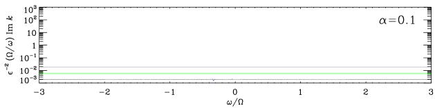
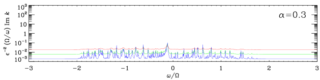
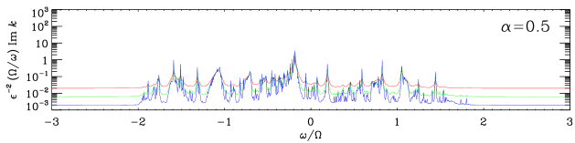
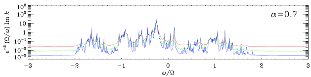
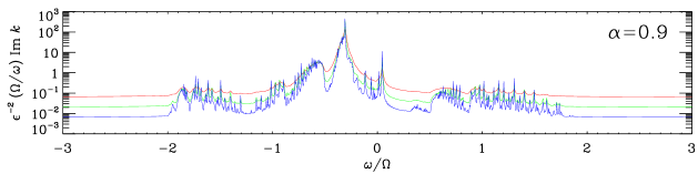
Figure 1: Frequency-dependent tidal response to $Y_{2}^{2}$ of a homogeneous body with an incompressible fluid envelope and a perfectly rigid solid core of fractional radius $\alpha=0.1$ (top panel), $0.3$, $0.5$, $0.7$ or $0.9$ (bottom panel). As in Ogilvie (2009) the fluid is inviscid but experiences a frictional force with a damping coefficient $\gamma$ given by $\gamma/\Omega=10^{-2}$ (red line), $10^{-2.5}$ (green line) or $10^{-3}$ (blue line); also, the surface is not free but has a prescribed radial motion. The imaginary part of the Love number is deduced from the dissipation rate and is plotted on a logarithmic scale after multiplication by $\epsilon^{-2}(\Omega/\omega)$, where $\Omega=\epsilon(GM/R^{3})^{1/2}$. A numerical resolution of $L=N=400$ is used.

Figure 2: Frequency-integral of the imaginary part of the Love number, weighted by $1/\omega$ and divided by $\epsilon^{2}$, for a homogeneous body, versus fractional core size. The solid line shows the analytical result (113) of the impulse calculation, while the symbols show the numerical integrals based on Figure 1 and similar calculations.

The divergence that occurs as $\alpha\to 1$ deserves some comment. The coefficient $C$ diverges in this limit, as do the non-radial components of the non-wavelike displacement. The thin, incompressible fluid shell is squeezed radially by the tidal force and produces rapid horizontal motion. Through the Coriolis force, a large wavelike velocity is also generated. This behaviour would be weakened if the core were not perfectly rigid but instead underwent some tidal deformation.

Generalizations of equation (113) can be found in Appendix B. In particular,

$$\int_{-\infty}^{\infty}\mathrm{Im}[K_{2}^{1}(\omega)]\,\frac{\mathrm{d}\omega}{\omega}=\frac{5\pi}{504}\epsilon^{2}\left(\frac{189+256\alpha^{5}}{1-\alpha^{5}}\right)$$ (114)

and

$$\int_{-\infty}^{\infty}\mathrm{Im}[K_{2}^{0}(\omega)]\,\frac{\mathrm{d}\omega}{\omega}=\frac{5\pi}{14}\epsilon^{2}\left(\frac{7+8\alpha^{5}}{1-\alpha^{5}}\right).$$ (115)

Note that, although these expressions are increasing functions of $\alpha$, they do not vanish at $\alpha=0$. We have also found excellent agreement between these expressions and the numerically integrated Love numbers using the method described above for the case $l=m=2$. The frequency-dependent responses are illustrated in Figures 3 and 4. Note that the enhancement of the tidal response in these cases results from resonances with the spin-over mode ($m=1$, $\omega/\Omega=-1$) and the spin-up mode ($m=0$, $\omega/\Omega=0$). These are trivial modes and there should be no associated dissipation. In these calculations the dissipation is artificial and results from the use of a frictional, rather than viscous, force. In either case, however, there is a formal singularity in $\mathrm{Im}\,k$ that gives a non-vanishing contribution to the integral even when $\alpha=0$. In a viscous fluid the resonance should be of zero width.

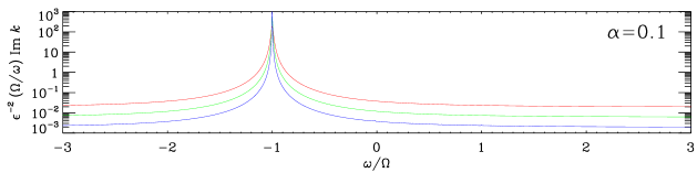
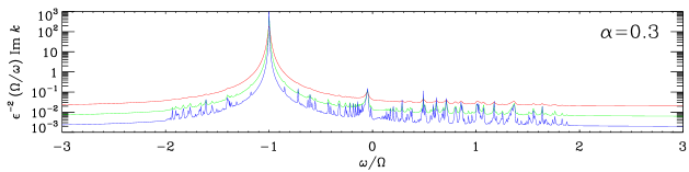
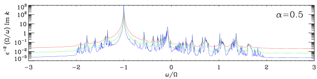
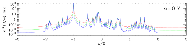
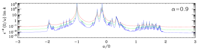
Figure 3: As for Figure 1 but for the tidal potential $Y_{2}^{1}$. There is a formal resonance with the spin-over mode at $\omega/\Omega=-1$.

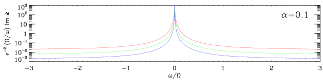
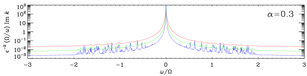
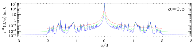
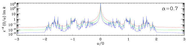
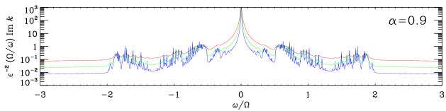
Figure 4: As for Figure 1 but for the tidal potential $Y_{2}^{0}$. There is a formal resonance with the spin-up mode at $\omega/\Omega=0$.

To illustrate the richer possibilities that exist for tidal potential components beyond the quadrupolar ones, we show similar results for $l=4$ and $m=1$ in Figure 5. In this case the response for small values of $\alpha$ is dominated by resonances with non-trivial inertial modes of the full sphere (at $\omega/\Omega=-1.7080$, $-0.6120$ and $+0.8200$, as expected from equation 15). For larger core sizes the frequency-dependence is qualitatively similar to that seen for quadrupolar tidal potentials. The analytical result in this case is

$$\int_{-\infty}^{\infty}\mathrm{Im}[K_{4}^{1}(\omega)]\,\frac{\mathrm{d}\omega}{\omega}=\frac{27\pi}{616000}\epsilon^{2}\left(\frac{6875+7168\alpha^{9}}{1-\alpha^{9}}\right).$$ (116)

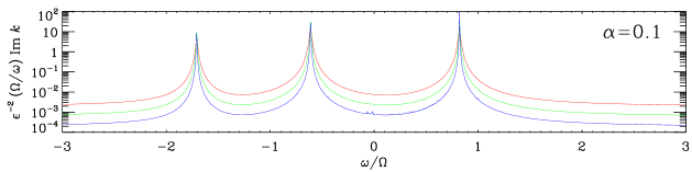
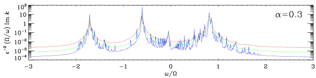
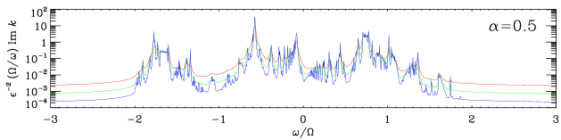
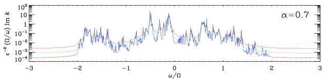
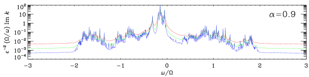
Figure 5: As for Figure 1 but for the tidal potential $Y_{4}^{1}$. This case is chosen to illustrate the richer response (for small core sizes) to tesseral harmonics of higher degrees. Note, however, the different scale on the vertical axis.

The integrated responses for all tidal potentials up to $l=4$ are shown in Figure 6. Although there is a general weakening of the response with increasing $l$, the integrated response to a tesseral harmonic of higher $l$ is usually much stronger than that to a sectoral harmonic of lower $l$.

4.9 Application to a piecewise-homogeneous fluid model

We now examine the effect of replacing the rigid solid core with a fluid core. We therefore consider a homogeneous fluid of density $\rho_{1}$ in $0<r<\alpha R$ and another of density $\rho_{2}$ in $\alpha R<r<R$, with $\rho_{1}\geq\rho_{2}$ for gravitational stability.

At an interface, where the density changes abruptly, $\xi_{\mathrm{nw},r}=-(\Phi^{\prime}+\Psi)/g$. This is because the Lagrangian pressure perturbation $p^{\prime}-\rho g\xi_{r}$ is continuous, but $p^{\prime}=\rho(W-\Phi^{\prime}-\Psi)$ and $W$ is supposed to be negligible [$O(\epsilon^{2})$] in the low-frequency approximation. If $\rho$ is discontinuous then we find the stated condition, which means that the interface moves equipotentially. (This should be valid provided that the tidal frequency is small compared to the relevant interfacial gravity wave frequency.)

The Helmholtz-like equation is then

$$\nabla^{2}\hat{\Phi}^{\prime}+\frac{4\pi G}{g}(\hat{\Phi}^{\prime}+\hat{\Psi})[(\rho_{1}-\rho_{2})\delta(r-\alpha R)+\rho_{2}\delta(r-R)]=0.$$ (117)

Given $\hat{\Psi}=A(r/R)^{l}Y_{l}^{m}$, the solution is $\hat{\Phi}^{\prime}=\hat{\Phi}^{\prime}_{l}(r)Y_{l}^{m}$, with

$$\hat{\Phi}^{\prime}_{l}=\left\{\begin{array}[]{ll}(B_{1}+B_{2})(r/R)^{l},&0<r<\alpha R,\\ B_{1}(r/R)^{l}+B_{2}\alpha^{2l+1}(R/r)^{l+1},&\alpha R<r<R,\\ (B_{1}+B_{2}\alpha^{2l+1})(R/r)^{l+1},&r>R,\end{array}\right.$$ (118)

where the coefficients satisfy the matching conditions

$$(2l+1)B_{2}=3(1-f)(A+B_{1}+B_{2}),$$ (119)

$$(2l+1)B_{1}=\frac{3f}{f+(1-f)\alpha^{3}}(A+B_{1}+B_{2}\alpha^{2l+1}),$$ (120)

with $f=\rho_{2}/\rho_{1}$. We shall not write explicitly the algebraic solution for $B_{1}$ and $B_{2}$.

$\hat{X}$ satisfies Laplace’s equation in each fluid shell and the solution (regular at $r=0$) is of the form

$$\hat{X}_{l}=\left\{\begin{array}[]{ll}C_{1}(r/R)^{l},&0<r<\alpha R,\\ C_{2}(r/R)^{l}+C_{3}\alpha^{2l+1}(R/r)^{l+1},&\alpha R<r<R.\end{array}\right.$$ (121)

The condition on the radial displacement is $\mathrm{d}\hat{X}_{l}/\mathrm{d}r=(\hat{\Phi}_{l}+\hat{\Psi}_{l})/g$ at each interface. Thus

$$lC_{1}=lC_{2}-(l+1)C_{3}=\frac{3(A+B_{1}+B_{2})}{4\pi G\rho_{1}},$$ (122)

$$lC_{2}-(l+1)C_{3}\alpha^{2l+1}=\frac{3(A+B_{1}+B_{2}\alpha^{2l+1})}{4\pi G(\rho_{2}+(\rho_{1}-\rho_{2})\alpha^{3})}.$$ (123)

The fact that $C_{3}\neq 0$ in general means that $\hat{X}_{l}$ is discontinuous in general at $r=\alpha R$. This means that the non-wavelike displacement has a tangential discontinuity. The singularity of vorticity results from the non-barotropic nature of the density jump.

$\hat{W}$ also satisfies Laplace’s equation and the solution is

$$\hat{W}_{l}=\left\{\begin{array}[]{ll}-2\mathrm{i}m\Omega(C_{1}/l)(r/R)^{l},\\ -2\mathrm{i}m\Omega[(C_{2}/l)(r/R)^{l}-(C_{3}/(l+1))\alpha^{2l+1}(R/r)^{l+1}],\end{array}\right.$$ (124)

such that

$$\hat{a}_{l}=\hat{b}_{l}=0.$$ (125)

(Here and below, the first and second cases of the expressions in braces apply for $0<r<\alpha R$ and $\alpha R<r<R$, respectively.) The toroidal part is given by

$$\hat{c}_{l-1}=\left\{\begin{array}[]{ll}-2\Omega\tilde{q}_{l}r^{-2}(2l+1)C_{1}(r/R)^{l},\\ -2\Omega\tilde{q}_{l}r^{-2}(2l+1)C_{2}(r/R)^{l},\end{array}\right.$$ (126)

$$\hat{c}_{l+1}=\left\{\begin{array}[]{ll}0,\\ -2\Omega\tilde{q}_{l+1}r^{-2}(2l+1)C_{3}\alpha^{2l+1}(R/r)^{l+1}.\end{array}\right.$$ (127)

The contributions to the impulse energy are then

$$\hat{E}_{l}=0,$$ (128)

$$\hat{E}_{l-1} = l(l-1)(2l+1)\Omega^{2}\tilde{q}_{l}^{2}$$ (129)

$$\times[\rho_{1}\alpha^{2l+1}|C_{1}|^{2}+\rho_{2}(1-\alpha^{2l+1})|C_{2}|^{2}]R,$$

$$\hat{E}_{l+1} = (l+1)(l+2)(2l+1)\Omega^{2}\tilde{q}_{l+1}^{2}$$ (130)

$$\times\rho_{2}\alpha^{2l+1}(1-\alpha^{2l+1})|C_{3}|^{2}R.$$

These results are converted into integrals of $\mathrm{Im}\,k$ using equation (76) and plotted in Figure 7 for various values of $f$ in the case $l=m=2$; the analytical result is given in equation (143). For small values of $f$ (large density contrasts) the impulsive response is similar to, but weaker than, the case of a homogeneous fluid with a solid core; the differences are greater when the core is larger. These results show that a fluid core can play a similar (if weaker) role in the excitation of inertial waves to that of a rigid solid core. As $f$ tends to $1$ the response disappears because the system becomes a full homogeneous sphere.

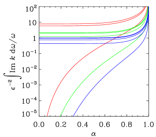
Figure 6: As for Figure 2 but showing only the results of the impulse calculation for a homogeneous body and for various tidal potentials with $l=2$ (red lines), $l=3$ (green lines) and $l=4$ (blue lines). On the left of the figure the ordering of curves is, from top to bottom: $Y_{2}^{0}$, $Y_{2}^{1}$, $Y_{3}^{0}$, $Y_{3}^{1}$, $Y_{3}^{2}$, $Y_{4}^{0}$, $Y_{4}^{1}$, $Y_{4}^{2}$, $Y_{4}^{3}$, $Y_{2}^{2}$, $Y_{3}^{3}$, $Y_{4}^{4}$.

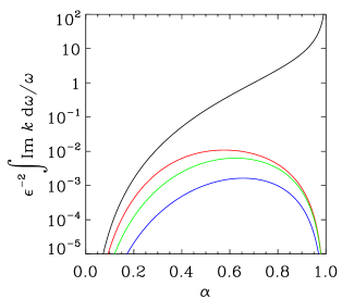
Figure 7: As for Figure 2 but showing only the results of the impulse calculation for a homogeneous body (black line) and for the piecewise-homogeneous fluid model with density ratio $f=0.25$ (red line), $f=0.5$ (green line) or $f=0.75$ (blue line).

4.10 Application to polytropes

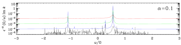
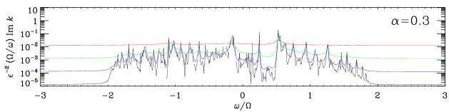
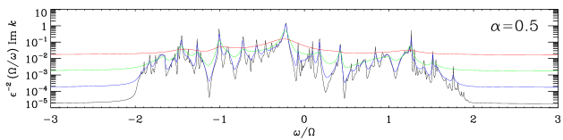
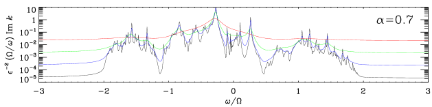
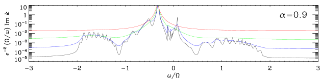
Figure 8: Frequency-dependent tidal response to $Y_{2}^{2}$ of an $n=1$ polytrope with a fluid envelope and a perfectly rigid solid core of fractional radius $\alpha=0.1$ (top panel), $0.3$, $0.5$, $0.7$ or $0.9$ (bottom panel). The fluid is viscous and the Ekman number is $\mathrm{Ek}=10^{-3}$ (red line), $10^{-4}$ (green line), $10^{-5}$ (blue line) or $10^{-6}$ (black line). The imaginary part of the Love number is computed directly and is plotted on a logarithmic scale after multiplication by $\epsilon^{-2}(\Omega/\omega)$, where $\Omega=\epsilon(GM/R^{3})^{1/2}$. In these calculations $\epsilon=0.01$ and the fluid envelope is truncated with a free surface at a fractional radius of $0.99$. A numerical resolution of $L=N=200$ is used. The results for $\mathrm{Ek}=10^{-6}$ are not fully converged at this resolution and occasionally return negative values of $\epsilon^{-2}(\Omega/\omega)\mathrm{Im}\,k$, resulting in gaps in the black line.

We have also computed the impulsive energy transfer $\hat{E}$ for polytropes of various indices $n$. This is done by first solving the Lane–Emden equation for the structure of the polytrope, then computing the impulsive response by solving the ODEs of Section 4.6 numerically by standard methods. We allow for a perfectly rigid solid core to be present, and assume that the mass of the core is equal to the mass of fluid that would occupy the equivalent region in a full polytrope.

The frequency-dependent response of an $n=1$ polytrope to $l=m=2$ tidal forcing is illustrated in Figure 8. These results are similar to those presented by Ogilvie & Lin (2004) but are computed by a different numerical method which will be described in forthcoming work (Ogilvie, in preparation). Rather than making a low-frequency approximation as in Ogilvie & Lin (2004), we solve the full set of linearized equations for a compressible, self-gravitating and viscous fluid while neglecting centrifugal effects (the parameter $\epsilon$ is here set to $0.01$). This method has the advantage that the Love number can be measured directly, because the gravitational potential perturbation is part of the numerical solution. The fluid is subject to viscous, rather than frictional, forces, as quantified by the Ekman number $\mathrm{Ek}=\nu/(2\Omega R^{2})$, where $\nu$ is the kinematic viscosity. In all cases except those at the lowest Ekman number $\mathrm{Ek}=10^{-6}$, where the numerical resolution may be insufficient, the imaginary part of the Love number is consistent with the viscous dissipation rate to a high degree of accuracy.

Figure 9: As for Figure 2 but for an $n=1$ polytrope. The numerical integrals are based on Figure 8 and similar calculations.

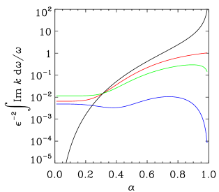
Figure 10: As for Figure 2 but showing only the results of the impulse calculation for a homogeneous body (black line) and for polytropes of indices $n=1$ (red line), $n=3/2$ (green line) and $n=3$ polytrope (blue line).

While there are many qualitative features in common between Figures 1 and 8, there are also important differences. For very small core sizes such as $\alpha=0.1$, the homogeneous body exhibits almost no response to $Y_{2}^{2}$, while the $n=1$ polytrope shows a few resonant peaks. These correspond to the resonant excitation of inertial normal modes of the full polytrope, which have been computed by Lockitch & Friedman (1999). Similar modes also exist in the homogeneous sphere, but they have no overlap with the $Y_{2}^{2}$ tidal potential and are not excited. For larger core sizes, normal modes cease to be important, until the limit of a thin shell is reached, in which the dominant feature is the excitation of a planetary wave/Rossby wave/r mode at $\omega/\Omega=-1/3$ (Ogilvie, 2009).

In Figure 9 we show the integrated quantity $\int\mathrm{Im}\,k\,\mathrm{d}\omega/\omega$, divided by $\epsilon^{2}$, as determined both from numerical integration of the curves in Figure 8 (and similar calculations) and from the impulse calculation described above. The two are in very good agreement, except in a few cases where the numerical integration probably has insufficient frequency-resolution to capture the narrow peaks that occur in $\mathrm{Im}\,k$ at low $\mathrm{Ek}$, or where the numerical resolution is insufficient to determine the dissipation rate accurately.

Figure 10 compares similar results (but without the numerically integrated values) for a homogeneous body and for polytropes of indices $n=1$, $3/2$ and $3$. This figure shows that, as the polytropic index increases and the body becomes more centrally condensed, the integrated tidal response to $Y_{2}^{2}$ becomes less sensitive to the size of the core. The main reason for this result is that the overlap between the $Y_{2}^{2}$ potential and the inertial normal modes of the full polytrope increases as $n$ increases, so that a significant tidal response (albeit concentrated into narrow peaks) is possible even in the absence of a core.

These results are in broad agreement with the findings of Papaloizou & Ivanov (2010), who calculated the energy transferred (predominantly to inertial waves) to a slowly rotating $n=1$ polytrope during a distant parabolic encounter. They found that the energy transferred via $Y_{2}^{2}$ was increased by nearly an order of magnitude when a (perfectly rigid) solid core with $\alpha=0.5$ was introduced, but hardly at all when $\alpha=0.25$. This is broadly in line with the red curve in Figure 10; although a parabolic encounter provides a tidal force that is localized in time, their problem is not identical to the impulse problem considered in this paper. For example, the Fourier transform of the Heaviside function has a singularity at zero frequency that is not present in the case of a parabolic encounter.

5 Conclusions

In this paper we have examined the linear response of slowly rotating, neutrally stratified astrophysical bodies to low-frequency tidal forcing. This problem may be regarded as a simplified model of tides in convective regions of stars and giant planets. The response can be separated into non-wavelike and wavelike parts, where the former is related instantaneously to the tidal potential and the latter may involve resonances or other singularities. The imaginary part of the potential Love number of the body, which is directly related to the rates of energy and angular momentum exchange in the tidal interaction and to the rate of dissipation of energy, may have a complicated dependence on the tidal frequency. However, a certain frequency-average of this quantity is independent of the dissipative properties of the fluid and can be determined by means of an impulse calculation. The result is a strongly increasing function of the size of the core when the tidal potential is a sectoral harmonic ($|m|=l$), such as the $l=m=2$ potential usually considered, especially when the body is not strongly centrally condensed. However, the same is not true for tesseral harmonics ($|m|<l$), which receive a richer response and may therefore be important in determining tidal evolution even though they are usually subdominant in the expansion of the tidal potential. We have also discussed analytically the low-frequency response of a slowly rotating homogeneous fluid body to tidal potentials proportional to spherical harmonics of degrees less than five. Tesseral harmonics of degrees greater than two, such as are present in the case of a spin-orbit misalignment, can resonate with inertial modes of the full sphere, leading to an enhanced tidal interaction. Similar behaviour can be expected in more realistic models.

The calculations carried out in this paper are based on linear theory and employ highly simplified interior structure models. There are various reasons why the complicated details of the frequency-dependent response functions might not be applicable to astrophysical bodies. The propagation of inertial waves may be impeded by nonlinearity (leading to instability, wave breaking, etc.), or interrupted by interactions with convection, magnetic fields, differential rotation, buoyancy forces, etc. The waves may not reflect perfectly from the boundaries of the convective regions that support them. These complications are likely to tend to wash out some of the structure in the frequency-dependent response curves. Nevertheless, the integrated response functions calculated in this paper are likely to be much more robust; they can be related, as we have seen, to the energy transferred in an impulsive interaction, which is independent of the detailed way in which the waves subsequently propagate, reflect and dissipate. The normal-mode resonances that we have identified with higher-order tidal potentials are also likely to be important even in the presence of effects such as convection.

Tidal interactions at low orbital eccentricity can be studied by analysing the tidal potential into a small number of components with a harmonic dependence on time. In this case the integrated responses discussed in this paper can be taken as indicative of the typical level of tidal dissipation, neglecting the complicated frequency-dependence associated with the propagation of inertial waves in a spherical shell. Of particular importance are the scaling of the imaginary part of the Love number (or the reciprocal of the tidal quality factor) with the square of the dimensionless rotation rate $\epsilon$, and its dependence on the size of a solid or fluid core that excludes the inertial waves by total or partial reflection. At high orbital eccentricity, tidal interactions are more impulsive in character because the tidal force is strongly peaked near pericentre, and the integrated responses are more directly applicable to such situations.

Previous works investigating tidally forced inertial waves in astrophysical bodies have tended to emphasize either global normal modes or the singular phenomena associated with wave attractors and critical latitudes. This paper attempts to bridge the gap between these descriptions. We consider that inviscid inertial waves in spherical (or spheroidal) geometry form true normal modes only under special conditions, i.e. when a core is absent and when the density profile is sufficiently smooth. We find classical resonances with normal modes in coreless homogeneous bodies and polytropes. As a core is introduced and increased in size, some ‘memory’ of these modes is retained initially, but later the singular wave phenomena dominate.

The application of these findings to extrasolar planets and solar-system bodies requires further work. The interior structure of giant planets is still quite uncertain; there may be non-smooth features such as discontinuities in the density or its radial derivative. Progress in the modelling of planetary interiors will certainly assist in the determination of their tidal responses.

Appendix A Responses of a homogeneous sphere

In this section we give some explicit solutions for the linear response of a slowly rotating homogeneous fluid body without a solid core to low-frequency tidal forcing. The notation follows that of Ogilvie (2009), with a time-dependence $\mathrm{e}^{-\mathrm{i}\omega t}$ in the frame rotating with the body, but viscous and frictional damping forces are omitted, so $\omega_{n}=\omega+2m\Omega/[n(n+1)]$.

Given $\Psi=A(r/R)^{l}Y_{l}^{m}$, the solution of the Helmholtz-like equation is, as in Section 4.8, $\Phi^{\prime}=B(r/R)^{l}Y_{l}^{m}$ for $r<R$ and $\Phi^{\prime}=B(R/r)^{l+1}Y_{l}^{m}$ for $r>R$, with $2(l-1)B=3A$. Then $X=C(r/R)^{l}Y_{l}^{m}$ with $C=(A+B)R/(lg)$ and $g=GM/R^{2}$. This gives $\xi_{\mathrm{nw},r}=aR(r/R)^{l-1}Y_{l}^{m}$, where $a=-lC/R^{2}$ is the dimensionless non-wavelike radial tidal amplitude at the surface. The non-wavelike velocity is given by

$$a_{l}=-\mathrm{i}\omega aR\left(\frac{r}{R}\right)^{l-1},\qquad b_{l}=-\mathrm{i}\omega\frac{a}{l}\left(\frac{r}{R}\right)^{l-2}.$$ (131)

The wavelike velocity solutions in various cases are as follows.

A.1 The case $l=2$

$$c_{1}=\frac{5aq_{2}\omega\Omega}{2\omega_{1}},\qquad W_{0}=\frac{5aq_{1}q_{2}\omega\Omega^{2}}{\omega_{1}}r^{2},\qquad W_{2}=\frac{a\omega\Omega(m\omega_{1}-5q_{2}^{2}\Omega)}{2\omega_{1}}r^{2}.$$ (132)

Note that a constant $c_{1}$, as occurs here, implies a special type of solution, not really an inertial wave. If $m=2$ this term vanishes because then $q_{2}=0$. If $m=1$ the term $c_{1}$ is a spin-over mode (tilting the rotation axis). If $m=0$ it is a spin-up mode (changing the rotation rate). The response is resonant when the denominator vanishes, i.e. when $\omega+m\Omega=0$, which means that the tidal frequency in the inertial frame vanishes.

A.2 The case $l=3$

$$a_{1}=\frac{14\mathrm{i}aq_{2}q_{3}\omega\Omega^{2}}{3(\omega_{1}\omega_{2}-3q_{2}^{2}\Omega^{2})}\frac{(R^{2}-r^{2})}{R},\qquad b_{1}=\frac{14\mathrm{i}aq_{2}q_{3}\omega\Omega^{2}}{3(\omega_{1}\omega_{2}-3q_{2}^{2}\Omega^{2})}\frac{(R^{2}-2r^{2})}{Rr},\qquad c_{2}=\frac{14aq_{3}\omega\omega_{1}\Omega}{9(\omega_{1}\omega_{2}-3q_{2}^{2}\Omega^{2})}\frac{r}{R}.$$ (133)

$$W_{1}=-\frac{14aq_{2}q_{3}\omega(\omega+2m\Omega)\Omega^{2}}{3(\omega_{1}\omega_{2}-3q_{2}^{2}\Omega^{2})}\frac{r(R^{2}-r^{2})}{R},\qquad W_{3}=a\omega\Omega\left[2m-\frac{56q_{3}^{2}\omega_{1}\Omega}{3(\omega_{1}\omega_{2}-3q_{2}^{2}\Omega^{2})}\right]\frac{r^{3}}{9R}.$$ (134)

The response is resonant when the common denominator vanishes, i.e. when

$$\omega=\frac{2}{3}\Omega\left[-m\pm\left(\frac{9-m^{2}}{5}\right)^{1/2}\right],$$ (135)

but not for $|m|=3$, because then $q_{3}$ in the numerator also vanishes.

A.3 The case $l=4$

$$a_{2}=\frac{81\mathrm{i}aq_{3}q_{4}\omega\omega_{1}\Omega^{2}}{9\omega_{1}\omega_{2}\omega_{3}-(27q_{2}^{2}\omega_{3}+32q_{3}^{2}\omega_{1})\Omega^{2}}\frac{r(R^{2}-r^{2})}{R^{2}},\qquad b_{2}=\frac{27\mathrm{i}aq_{3}q_{4}\omega\omega_{1}\Omega^{2}}{9\omega_{1}\omega_{2}\omega_{3}-(27q_{2}^{2}\omega_{3}+32q_{3}^{2}\omega_{1})\Omega^{2}}\frac{(3R^{2}-5r^{2})}{2R^{2}},$$ (136)

$$c_{1}=-\frac{81aq_{2}q_{3}q_{4}\omega\Omega^{3}}{9\omega_{1}\omega_{2}\omega_{3}-(27q_{2}^{2}\omega_{3}+32q_{3}^{2}\omega_{1})\Omega^{2}}\frac{(5R^{2}-7r^{2})}{2R^{2}},\qquad c_{3}=\frac{81aq_{4}\omega\Omega(\omega_{1}\omega_{2}-3q_{2}^{2}\Omega^{2})}{9\omega_{1}\omega_{2}\omega_{3}-(27q_{2}^{2}\omega_{3}+32q_{3}^{2}\omega_{1})\Omega^{2}}\frac{r^{2}}{8R^{2}},$$ (137)

$$W_{0}=-\frac{81aq_{1}q_{2}q_{3}q_{4}\omega\Omega^{4}}{9\omega_{1}\omega_{2}\omega_{3}-(27q_{2}^{2}\omega_{3}+32q_{3}^{2}\omega_{1})\Omega^{2}}\frac{r^{2}(10R^{2}-7r^{2})}{2R^{2}},\qquad W_{2}=-\frac{81aq_{3}q_{4}\omega\Omega^{2}(\omega_{1}^{2}-5q_{2}^{2}\Omega^{2})}{9\omega_{1}\omega_{2}\omega_{3}-(27q_{2}^{2}\omega_{3}+32q_{3}^{2}\omega_{1})\Omega^{2}}\frac{r^{2}(R^{2}-r^{2})}{2R^{2}},$$ (138)

$$W_{4}=a\omega\Omega\left[2m-\frac{243q_{4}^{2}\Omega(\omega_{1}\omega_{2}-3q_{2}^{2}\Omega^{2})}{9\omega_{1}\omega_{2}\omega_{3}-(27q_{2}^{2}\omega_{3}+32q_{3}^{2}\omega_{1})\Omega^{2}}\right]\frac{r^{4}}{16R^{2}}.$$ (139)

Again, the response is resonant when the common denominator vanishes, i.e. when $\omega$ satisfies the cubic equation

$$42\omega^{3}+63m\omega^{2}\Omega-36(2-m^{2})\omega\Omega^{2}-4m(11-2m^{2})\Omega^{3}=0,$$ (140)

but not for $|m|=4$, because then $q_{4}$ in the numerator also vanishes.

Appendix B Analytical results for integrated responses

B.1 Homogeneous body with a solid core

The equivalent of equation (113) for general values of $l$ and $m$ is

$$\int_{-\infty}^{\infty}\mathrm{Im}[K_{l}^{m}(\omega)]\,\frac{\mathrm{d}\omega}{\omega}=\frac{3(2l+1)\pi\epsilon^{2}[(l+1)^{3}(l-1)(2l+3)(l^{2}-m^{2})+l^{3}(l+2)(2l-1)((l+1)^{2}-m^{2})\alpha^{2l+1}]}{l^{3}(l+1)^{3}(l-1)^{2}(2l+3)(2l-1)(1-\alpha^{2l+1})}.$$ (141)

B.2 Homogeneous fluid body with a solid core of a different density

The equivalent result in the case $l=m=2$ when the solid core has a density $f^{-1}$ times that of the fluid envelope is

$$\int_{-\infty}^{\infty}\mathrm{Im}[K_{2}^{2}(\omega)]\,\frac{\mathrm{d}\omega}{\omega}=\frac{100\pi}{63}\epsilon^{2}\left(\frac{\alpha^{5}}{1-\alpha^{5}}\right)\left[1+\left(\frac{1-f}{f}\right)\alpha^{3}\right]\left[1+\frac{5}{2}\left(\frac{1-f}{f}\right)\alpha^{3}\right]^{-2}.$$ (142)

We recover equation (113) either as $f\to 1$ or in the limit $\alpha^{3}\ll f$.

B.3 Piecewise-homogeneous fluid body

The equivalent result for the piecewise-homogeneous fluid model is

$$\int_{-\infty}^{\infty}\mathrm{Im}[K_{2}^{2}(\omega)]\,\frac{\mathrm{d}\omega}{\omega} = \frac{100\pi}{63}\epsilon^{2}\left(\frac{\alpha^{5}}{1-\alpha^{5}}\right)(1-f)^{2}(1-\alpha)^{4}\left(1+2\alpha+3\alpha^{2}+\frac{3}{2}\alpha^{3}\right)^{2}\left[1+\left(\frac{1-f}{f}\right)\alpha^{3}\right]$$ (143)

$$\times\left[1+\frac{3}{2}f+\frac{5}{2f}\left(1+\frac{1}{2}f-\frac{3}{2}f^{2}\right)\alpha^{3}-\frac{9}{4}(1-f)\alpha^{5}\right]^{-2}.$$

For small $f$ and small $\alpha$, specifically $\alpha^{3}\ll f\ll 1$, we again recover equation (113).

References

- Albrecht et al. (2012) Albrecht S., et al., 2012, arXiv, arXiv:1206.6105
- Alexander (1973) Alexander M. E., 1973, Ap&SS, 23, 459
- Barker & Ogilvie (2009) Barker A. J., Ogilvie G. I., 2009, MNRAS, 395, 2268
- Barker & Ogilvie (2010) Barker A. J., Ogilvie G. I., 2010, MNRAS, 404, 1849
- Bryan (1889) Bryan G. H., 1889, Philos. Trans. R. Soc. London, A180, 187
- Chandrasekhar (1969) Chandrasekhar S., 1969, Ellipsoidal Figures of Equilibrium, Yale Univ. Press, New Haven
- Darwin (1880) Darwin G. H., 1880, RSPT, 171, 713
- Eggleton, Kiseleva & Hut (1998) Eggleton P. P., Kiseleva L. G., Hut P., 1998, ApJ, 499, 853
- Goldreich (1963) Goldreich P., 1963, MNRAS, 126, 257
- Goldreich & Nicholson (1989) Goldreich P., Nicholson P. D., 1989, ApJ, 342, 1079
- Goldreich & Soter (1966) Goldreich P., Soter S., 1966, Icarus, 5, 375
- Goodman & Dickson (1998) Goodman J., Dickson E. S., 1998, ApJ, 507, 938
- Goodman & Lackner (2009) Goodman J., Lackner C., 2009, ApJ, 696, 2054
- Greenspan (1968) Greenspan H. P., 1968, The Theory of Rotating Fluids, Cambridge Univ. Press, Cambridge
- Hut (1981) Hut P., 1981, A&A, 99, 126
- Jeffreys (1961) Jeffreys H., 1961, MNRAS, 122, 339
- Lai (2012) Lai D., 2012, MNRAS, 423, 486
- Lapwood & Usami (1981) Lapwood E. R., Usami T., 1981, Free Oscillations of the Earth, Cambridge Univ. Press, Cambridge
- Lockitch & Friedman (1999) Lockitch K. H., Friedman J. L., 1999, ApJ, 521, 764
- Mardling & Lin (2002) Mardling R. A., Lin D. N. C., 2002, ApJ, 573, 829
- Mignard (1980) Mignard F., 1980, M&P, 23, 185
- Morse & Feshbach (1953) Morse P. M., Feshbach H., 1953, Methods of Theoretical Physics, McGraw-Hill, New York
- Ogilvie (2005) Ogilvie G. I., 2005, J. Fluid Mech., 543, 19
- Ogilvie (2009) Ogilvie G. I., 2009, MNRAS, 396, 794
- Ogilvie & Lin (2004) Ogilvie G. I., Lin D. N. C., 2004, ApJ, 610, 477
- Ogilvie & Lin (2007) Ogilvie G. I., Lin D. N. C., 2007, ApJ, 661, 1180
- Papaloizou & Ivanov (2005) Papaloizou J. C. B., Ivanov P. B., 2005, MNRAS, 364, L66
- Papaloizou & Ivanov (2010) Papaloizou J. C. B., Ivanov P. B., 2010, MNRAS, 407, 1631
- Papaloizou & Savonije (1997) Papaloizou J. C. B., Savonije G. J., 1997, MNRAS, 291, 651
- Rieutord & Valdettaro (2010) Rieutord M., Valdettaro L., 2010, J. Fluid Mech., 643, 363
- Savonije & Papaloizou (1983) Savonije G. J., Papaloizou J. C. B., 1983, MNRAS, 203, 581
- Savonije & Papaloizou (1997) Savonije G. J., Papaloizou J. C. B., 1997, MNRAS, 291, 633
- Savonije, Papaloizou & Alberts (1995) Savonije G. J., Papaloizou J. C. B., Alberts F., 1995, MNRAS, 277, 471
- Savonije & Witte (2002) Savonije G. J., Witte M. G., 2002, A&A, 386, 211
- Smeyers (2010) Smeyers P., 2010, Linear Isentropic Oscillations of Stars, Springer, Heidelberg
- Terquem et al. (1998) Terquem C., Papaloizou J. C. B., Nelson R. P., Lin D. N. C., 1998, ApJ, 502, 788
- Thomson (1863) Thomson W., 1863, Philos. Trans. R. Soc. London, 153, 583
- Witte & Savonije (1999) Witte M. G., Savonije G. J., 1999, A&A, 341, 842
- Wu (2005a) Wu Y., 2005a, ApJ, 635, 674
- Wu (2005b) Wu Y., 2005b, ApJ, 635, 688
- Zahn (1966a) Zahn J. P., 1966a, AnAp, 29, 313
- Zahn (1977) Zahn J.-P., 1977, A&A, 57, 383