Discussion: Latent variable graphical model selection via convex optimization

10.1214/11-AOS949

and

Recently there has been an increasing interest in the problem of estimating a high-dimensional matrix $K$ that can be decomposed in a sum of a sparse matrix $S^{*}$ (i.e., a matrix having only a small number of nonzero entries) and a low rank matrix $L^{*}$. This is motivated by applications in computer vision, video segmentation, computational biology, semantic indexing, etc. The main contribution and novelty of the Chandrasekaran, Parrilo and Willsky paper (CPW in what follows) is to propose and study a method of inference about such decomposable matrices for a particular setting where $K$ is the precision (concentration) matrix of a partially observed sparse Gaussian graphical model (GGM). In this case, $K$ is the inverse of the covariance matrix of a Gaussian vector $X_{O}$ extracted from a larger Gaussian vector $(X_{O},X_{H})$ with sparse inverse covariance matrix. Then it is easy to see that $K$ can be represented as a sum of a sparse precision matrix $S^{*}$ corresponding to the observed variables $X_{O}$ and a matrix $L^{*}$ with rank at most $h$, where $h$ is the dimension of the latent variables $X_{H}$. If $h$ is small, which is a typical situation in practice, then $L^{*}$ has low rank. The GGM with latent variables is of major interest for applications in biology or in social networks where one often does not observe all the variables relevant for depicting sparsely the conditional dependencies. Note that formally this is just one possible motivation and mathematically the problem is dealt with in more generality, namely, postulating that the precision matrix satisfies

$$K=S^{*}+L^{*}$$ (1)

with sparse $S^{*}$ and low-rank $L^{*}$, both symmetric matrices. A small amendment to that inherited from the latent variables motivation is that $L^{*}$ is assumed negative definite (in our notation, $L^{*}$ corresponds to $-L^{*}$ in the paper). We believe that this is not crucial and all the results remain valid without this assumption.

CPW propose to estimate the pair $(S^{*},L^{*})$ from a $n$-sample of $X_{O}$ by the pair $(\widehat{S},\widehat{L})$ obtained by minimizing the negative log-likelihood with mixed $\ell^{1}$ and nuclear norm penalties; cf. (1.2) of the paper. The key issue in this context is identifiability. Under what conditions can we identify $S^{*}$ and $L^{*}$ separately? CPW provide geometric conditions of identifiability based on transversality of tangent spaces to the varieties of sparse and low-rank matrices. They show that, under these conditions, with probability close to 1, it is possible to recover the support of $S^{*}$, the rank of $L^{*}$ and to get a bound of order $O(\sqrt{p/n})$ on the estimation errors $|\widehat{S}-S^{*}|_{\ell^{\infty}}$ and $\|\widehat{L}-L^{*}\|_{2}$. Here, $p$ is the dimension of $X_{O}$ and $|\cdot|_{\ell^{q}}$ and $\|\cdot\|_{2}$ stand for the componentwise $\ell^{q}$-norm and the spectral norm of a matrix, respectively.

Overall, CPW pioneer a hard and important problem of high-dimensional statistics and provide an original solution both in the theory and in numerically implementable realization. While being the first work to shed light on the problem, the paper does not completely raise the curtain and several aspects still remain to be understood and elucidated.

The nature of the results

The most important problem for current applications appears to be the estimation of $S^{*}$ or the recovery of its support. Indeed, the main interest is in the conditional dependencies of the coordinates of $X_{O}$ in the complete model $(X_{O},X_{H})$ and this information is carried by the matrix $S^{*}$. In this context, $L^{*}$ is essentially a nuisance, so that bounds on the estimation error of $L^{*}$ and the recovery of the rank of $L^{*}$ are of relatively moderate interest. However, mathematically, the most sacrifice comes from the desire to have precise estimates of $L^{*}$. Indeed, if $\widehat{\Sigma}_{n}$ and $\Sigma$ denote the empirical and population covariance matrices, the slow rate $O(\sqrt{p/n})$ comes from the bound on $\|\widehat{\Sigma}_{n}-\Sigma\|_{2}$ in Lemma 5.4, that is, from the stochastic error corresponding to $L^{*}$. Since the sup-norm error $|\widehat{\Sigma}_{n}-\Sigma|_{\ell^{\infty}}$ is of order $\sqrt{(\log p)/n}$, can we get a better rate when solely focusing on $|\widehat{S}-S^{*}|_{\ell^{\infty}}$?

Extension to high dimensions

The results of the paper are valid and meaningful only when $p<n$. However, for the applications of GGM, the case $p\gg n$ is the most common. A key question is whether the restriction $p<n$ is intrinsic, that is, whether it is possible to have results on $S^{*}$ in model (1) when $p\gg n$. Since the traditional model with sparse component $S^{*}$ alone is still tractable when $p\gg n$, a related question is whether introducing the model (1) with two components and estimating both $S^{*}$ and $L^{*}$ gives any improvement in the $p\gg n$ setting as compared to estimation in the model with a sparse component alone. A small simulation study that we provide below suggests that already for $p=n,$ including the low-rank component in the estimator may yield no improvement as compared to traditional sparse estimation without the low-rank component, although this low-rank component is effectively present in the model.

Optimal rates

The paper obtains bounds of order $O(\sqrt{p/n})$ on the estimation errors $|\widehat{S}-S^{*}|_{\ell^{\infty}}$ and $\|\widehat{L}-L^{*}\|_{2}$ with probability $1-2\exp(-p)$. Can we achieve a better rate than $\sqrt{p/n}$ when solely focusing on the recovery of $S^{*}$ with the usual probability $1-p^{-a}$ for some $a>0$? Is the rate $\sqrt{p/n}$ optimal in a minimax sense on some class of matrices? Note that one should be careful in defining the class of matrices because in reality the rate is not $O(\sqrt{p/n})$ but rather $O(\psi\sqrt{p/n})$, where $\psi$ is the spectral norm of $\Sigma$ depending on $p$. It can be large for large $p$. Surprisingly, not much is known about the optimal rates even in the simpler case of purely sparse precision matrices, without the low-rank component. In this case, RavikumarEtal , cai_etal and sun_zhang provide some analysis of the upper bounds on the estimation error of different estimators and under different sets of assumptions on the precision matrix. All these bounds are of “order” $O(\sqrt{(\log p)/n})$, but again one should be very careful here because of the factors depending on $p$ that multiply this rate. In cai_etal , the factor is the squared $\ell^{1}\to\ell^{1}$ norm of the precision matrix while in RavikumarEtal , it is the squared degree of the graphical model multiplied by some combinations of powers of matrix norms that are not easy to interpret. The most recent paper sun_zhang obtains the rate $O(d\sqrt{(\log p)/n})$, where $d$ is the degree of the graph for $\ell^{\infty}$-bounded precision matrices. An open problem is to find optimal rates of convergence on classes of precision matrices defined via sparsity and low rank characteristics. The same problem makes sense for covariance matrices. Here, some advances have been achieved very recently. In particular, some optimal rates of estimation of low-rank covariance matrices are provided by Lounici .

The assumptions of the paper are stated in terms of some inaccessible characteristics such as $\xi(T)$ and $\mu(\Omega)$ and seem to be very strong. They are in the spirit of the irrepresentability condition for the vector case used to prove model selection consistency of the Lasso. For a given set of data, there is no means to check whether these assumptions are satisfied. What happens when they do not hold? Can we still have some convergence properties under no assumption at all or under weaker assumptions akin to the restricted eigenvalue condition in the vector case?

Choice of the tuning parameters

The choice of parameters $(\gamma,\lambda_{n})$ ensuring algebraic consistency in Theorem 4.1 depends on various unknown quantities. Proposing a reasonable data-driven selector for $(\gamma,\lambda_{n})$ (e.g., similarly to GHV12 for the pure sparse setting) would be very helpful for the practice.

Alternative methods of estimation

Constructively, the method of CPW is obtained from the GLasso of FHT by adding a penalization by the nuclear norm of the low-rank component. Similar low-rank extensions can be readily derived from other methods, such as the Dantzig type approach of cai_etal and the regression approach of MB06 , Gir08 . Consider a Gaussian random vector $X\in\mathbb{R}^{p}$ with mean 0 and nonsingular covariance matrix $\Sigma$. Let $K=\Sigma^{-1}$ be the precision matrix. We assume that $K$ is of the form (1) where $S^{*}$ is sparse and $L^{*}$ has low rank.

(a) Dantzig type approach. In the spirit of cai_etal , we may define our estimator as a solution of the following convex program:

$$(\widehat{S},\widehat{L})=\operatorname{argmin}\limits_{(S,L)\in\mathcal{G}}\{|S|_{\ell^{1}}+\mu\|L\|_{*}\},$$ (2)

where $\|\cdot\|_{*}$ is the nuclear norm, $\mathcal{G}=\{(S,L)\dvtx|\widehat{\Sigma}_{n}(S+L)-I|_{\ell^{\infty}}\leq\lambda\}$ and $\mu,\lambda>0$ are tuning constants. Here, the nuclear norm $\|L\|_{*}$ is a convex relaxation of the rank of $L^{*}$.

(b) Regression approach. The regression approach MB06 , Gir08 is an alternative point of view for estimating the structure of a GGM. In the pure sparse setting, some numerical experiments VillersEtal suggest that it may be more reliable than the $\ell^{1}$-penalized log-likelihood approach. Let $\operatorname{diag}(A)$ denote the diagonal of square matrix $A$ and $\|A\|_{F}$ its Frobenius norm. Defining

$$\Theta=\operatorname{argmin}\limits_{A:\operatorname{diag}(A)=0}\|\Sigma^{1/2}(I-A)\|_{F}^{2},$$

we have $\Theta=K\Delta+I$, where $I$ is the identity matrix and $\Delta$ is the diagonal matrix with diagonal elements $\Delta_{jj}=-1/K_{jj}$ for $j=1,\ldots,p$. Thus, we have the decomposition

$$\Theta=\bar{S}+\bar{L},\qquad\mbox{where }\bar{S}=S^{*}\Delta+I\ \mbox{ and }\bar{L}=L^{*}\Delta.$$

Note that $\operatorname{rank}(\bar{L})=\operatorname{rank}(L^{*})$ and the nondiagonal elements $\bar{S}_{ij}$ of matrix $\bar{S}$ are nonzero only if $S^{*}_{ij}$ is nonzero. Therefore, recovering the support of $S^{*}$ and $\operatorname{rank}(L^{*})$ is equivalent to recovering the support of $\bar{S}$ and $\operatorname{rank}(\bar{L})$.

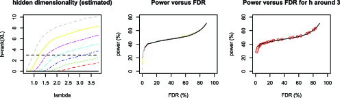
Figure 1: Each color corresponds to a fixed value of $\mu$, the solid-black color being for $\mu=+\infty$. For each choice of $\mu$, different quantities are plotted for a series of values of $\lambda$. Left: Mean rank of $\mathbf{X}\widehat{L}$. Middle: The curve of estimated power versus estimated FDR. Right: The power versus FDR for the estimators fulfilling $\mathbb{E}[\operatorname{rank}(\mathbf{X}\widehat{L})]\approx h=3$ (red dots), superposed with the Power versus the FDR for $\mu=+\infty$ (in solid-black).

Now, we estimate $(\bar{S},\bar{L})$ from an $n$-sample of $X$ represented as an $n\times p$ matrix $\mathbf{X}$. Noticing that the sample analog of $\|\Sigma^{1/2}(I-A)\|_{F}^{2}$ is $\|\mathbf{X}(I-A)\|_{F}^{2}/n$ and using the decomposition $\Theta=\bar{S}+\bar{L}$, we arrive at the following estimator:

$$\hskip 10.0pt(\widehat{S},\widehat{L})=\operatorname{argmin}\limits_{(S,L):\operatorname{diag}(S+L)=0}\biggl{\{}\frac{1}{2}\|\mathbf{X}(I-S-L)\|_{F}^{2}+\lambda|S|_{\ell^{1},\mathrm{off}}+\mu\|\mathbf{X}L\|_{*}\biggr{\}},$$ (3)

where $\mu,\lambda$ are positive tuning constants and $|S|_{\ell^{1},\mathrm{off}}=\sum_{i\neq j}|S_{ij}|$. Note that here the low-rank shrinkage is driven by the nuclear norm $\|\mathbf{X}L\|_{*}$ rather than by $\|L\|_{*}$. The convex minimization in (3) can be performed efficiently by alternating block descents on the off-diagonal elements of $S$, the matrix $L$ and the diagonal of $S$. The off-diagonal support of $S^{*}$ is finally estimated by the off-diagonal support of $\widehat{S}$.

Numerical experiment

A sparse Gaussian graphical model in $\mathbb{R}^{30}$ is generated randomly according to the procedure described in Section 4 of GHV12 . A sample of size $n=30$ is drawn from this distribution and $\mathbf{X}$ is obtained by hiding the values of 3 variables. These 3 hidden variables are chosen randomly among the connected variables. The estimators $(\widehat{S},\widehat{L})$ defined in (3) are then computed for a grid of values of $\lambda$ and $\mu$. The results are summarized in Figure 1 (average over 100 simulations).

Strikingly, there is no significative difference in these examples between the procedure of MB06 (corresponding to $\mu=+\infty$, in solid-black) and the procedure (3) that includes the low-rank component (corresponding to finite $\mu$).

References

- (1) {barticle}[mr] \bauthor\bsnmCai, \bfnmTony\binitsT., \bauthor\bsnmLiu, \bfnmWeidong\binitsW. and \bauthor\bsnmLuo, \bfnmXi\binitsX. (\byear2011). \btitleA constrained minimization approach to sparse precision matrix estimation. \bjournalJ. Amer. Statist. Assoc. \bvolume106 \bpages594–607. \biddoi=10.1198/jasa.2011.tm10155, issn=0162-1459, mr=2847973 \bptokimsref \endbibitem
- (2) {barticle}[auto:STB—2012/06/01—15:11:24] \bauthor\bsnmFriedman, \bfnmJ.\binitsJ., \bauthor\bsnmHastie, \bfnmT.\binitsT. and \bauthor\bsnmTibshirani, \bfnmR.\binitsR. (\byear2007). \btitleSparse inverse covariance estimation with the graphical Lasso. \bjournalBiostatistics \bvolume9 \bpages432–441. \bptokimsref \endbibitem
- (3) {barticle}[mr] \bauthor\bsnmGiraud, \bfnmChristophe\binitsC. (\byear2008). \btitleEstimation of Gaussian graphs by model selection. \bjournalElectron. J. Stat. \bvolume2 \bpages542–563. \biddoi=10.1214/08-EJS228, issn=1935-7524, mr=2417393 \bptokimsref \endbibitem
- (4) {barticle}[auto:STB—2012/06/01—15:11:24] \bauthor\bsnmGiraud, \bfnmC.\binitsC., \bauthor\bsnmHuet, \bfnmS.\binitsS. and \bauthor\bsnmVerzelen, \bfnmN.\binitsN. (\byear2012). \btitleGraph selection with GGMselect. \bjournalStat. Appl. Genet. Mol. Biol. \bvolume11 \bpages1–50. \bptokimsref \endbibitem
- (5) {bmisc}[auto:STB—2012/06/01—15:11:24] \bauthor\bsnmLounici, \bfnmK.\binitsK. (\byear2012). \bhowpublishedHigh-dimensional covariance matrix estimation with missing observations. Available at arXiv:\arxivurl1201.2577. \bptokimsref \endbibitem
- (6) {barticle}[mr] \bauthor\bsnmMeinshausen, \bfnmNicolai\binitsN. and \bauthor\bsnmBühlmann, \bfnmPeter\binitsP. (\byear2006). \btitleHigh-dimensional graphs and variable selection with the lasso. \bjournalAnn. Statist. \bvolume34 \bpages1436–1462. \biddoi=10.1214/009053606000000281, issn=0090-5364, mr=2278363 \bptokimsref \endbibitem
- (7) {barticle}[mr] \bauthor\bsnmRavikumar, \bfnmPradeep\binitsP., \bauthor\bsnmWainwright, \bfnmMartin J.\binitsM. J., \bauthor\bsnmRaskutti, \bfnmGarvesh\binitsG. and \bauthor\bsnmYu, \bfnmBin\binitsB. (\byear2011). \btitleHigh-dimensional covariance estimation by minimizing -penalized log-determinant divergence. \bjournalElectron. J. Stat. \bvolume5 \bpages935–980. \biddoi=10.1214/11-EJS631, issn=1935-7524, mr=2836766 \bptokimsref \endbibitem
- (8) {bmisc}[auto:STB—2012/06/01—15:11:24] \bauthor\bsnmSun, \bfnmT.\binitsT. and \bauthor\bsnmZhang, \bfnmC. H.\binitsC. H. (\byear2012). \bhowpublishedSparse matrix inversion with scaled lasso. Available at arXiv:\arxivurl1202.2723. \bptokimsref \endbibitem
- (9) {barticle}[mr] \bauthor\bsnmVillers, \bfnmFanny\binitsF., \bauthor\bsnmSchaeffer, \bfnmBrigitte\binitsB., \bauthor\bsnmBertin, \bfnmCaroline\binitsC. and \bauthor\bsnmHuet, \bfnmSylvie\binitsS. (\byear2008). \btitleAssessing the validity domains of graphical Gaussian models in order to infer relationships among components of complex biological systems. \bjournalStat. Appl. Genet. Mol. Biol. \bvolume7 \bpagesArt. 14, 36. \biddoi=10.2202/1544-6115.1371, issn=1544-6115, mr=2465331 \bptokimsref \endbibitem