Volume dependence in 2+1 Yang-Mills theory

Abstract:

We present the results of an analysis of a 2+1 dimensional pure SU($N$) Yang-Mills theory formulated on a 2-dimensional spatial torus with non-trivial magnetic flux. We focus on investigating the dependence of the electric-flux spectrum, extracted from Polyakov loop correlators, with the spatial size $l$, the number of colours $N$, and the magnetic flux $m$. The size of the torus acts a parameter that allows to control the onset of non-perturbative effects. In the small volume regime, where perturbation theory holds, we derive the one-loop self-energy correction to the single-gluon spectrum, for arbitrary $N$ and $m$. We discuss the transition from small to large volumes that has been investigated by means of Monte-Carlo simulations. We argue that the energy of electric flux $\vec{e}$, for the lowest gluon momentum, depends solely on $\vec{e}/N$ and the dimensionless variable $x=\lambda Nl$, with $\lambda=g^{2}N$ the ’t Hooft coupling. The variable $x$ can be interpreted as the dimensionless ’t Hooft coupling for an effective box size given by $Nl$. This implies a version of reduction that allows to trade $l$ by $N$ without modifying the electric-flux energy.

1 Introduction

In this paper we will explore the electric-flux spectrum of a 2+1-dimensional SU(N) Yang-Mills theory defined on a 2-dimensional spatial torus endowed with a chromo-magnetic flux. The aim is to disentangle the dependence on the number of colours $N$ and the size of the torus $l$, following the idea of reduction introduced by Eguchi and Kawai [1, 2]. The size of the torus will act as a control parameter that permits to explore the onset of non-perturbative dynamics. This is so, because for small $l$ the effective coupling constant becomes small and perturbation theory holds. As $l$ grows, the finite size effects, including the magnetic flux, should become irrelevant. The way in which this takes place, and in particular the interplay with the large $N$ limit, might shed some light into the processes relevant for non-perturbative dynamics. We will focus here for simplicity on the 2+1 dimensional case that shares many of the non-perturbative properties of the 4-dimensional theory. There is an extensive literature on the subject of Yang-Mills 3-d fields and large $N$ dynamics, for recent lattice reviews we refer the reader to [3].

2 Set-up and Perturbative Analysis

We will be considering SU($N$) Yang-Mills theories defined on a spatial torus of size $l\times l$. In the basis of constant transition matrices $\Gamma_{i}$, the gauge field connection has to satisfy the periodicity condition: $A_{i}(x+l\hat{\jmath})=\Gamma_{j}A_{i}(x)\Gamma^{\dagger}_{j}$ , with the $\Gamma_{i}$ fulfilling:

$$\Gamma_{1}\Gamma_{2}=\exp\Big{\{}i\,{2\pi m\over N}\Big{\}}\,\,\Gamma_{2}\Gamma_{1}\quad,$$ (1)

where $m$ is the magnetic flux. In the case that $m$ and $N$ are co-prime, this equation defines the matrices $\Gamma_{i}$ uniquely modulo global gauge transformations. For simplicity we will assume that $N$ is odd and co-prime with $m$ in the following. The periodicity constraint on the gauge fields can be solved by introducing a basis of $N\times N$ matrices $\hat{\Gamma}({\vec{p}\,}^{c})$ satisfying:

$$\Gamma_{i}\hat{\Gamma}({\vec{p}\,}^{c})\Gamma_{i}^{\dagger}=e^{il{p}_{i}^{\,c}}\hat{\Gamma}({\vec{p}\,}^{c})\quad,$$ (2)

where ${\vec{p}\,}^{c}=\frac{2\pi\vec{n}}{lN}$, with $n_{i}$ integers defined modulo N. Thus, there are $N^{2}$ such matrices. An explicit solution to the equation is:

$$\hat{\Gamma}({\vec{p}\,}^{c})=e^{i\alpha({\vec{p}\,}^{c})}\,\,\Gamma_{1}^{\,-\,\bar{k}n_{2}}\,\Gamma_{2}^{\,\bar{k}\,n_{1}}\quad,$$ (3)

where $\bar{k}$ is an integer satisfying $m\bar{k}=1\bmod N$, and $\alpha({\vec{p}\,}^{c})$ an arbitrary phase factor. In this basis we can Fourier decompose the gauge connection as:

$$A_{i}(x)={\cal N}\,\sum^{\prime}_{\vec{P}}\,e^{i\vec{P}\vec{x}}\,\hat{A}_{i}(\vec{P})\,\hat{\Gamma}(\vec{P})\quad.$$ (4)

The total momentum $\vec{P}$ is quantized in units of $2\pi/(Nl)$ and can be decomposed as: $\vec{P}=\vec{p}+{\vec{p}\,}^{c}$, with $\vec{p}=2\pi\vec{n}/l$, and $n_{i}\in Z\!\!\!Z$. The prime means that ${\vec{p}\,}^{c}=\vec{0}$ is excluded from the sum, since $A_{i}(x)$ has to be traceless. This can be interpreted by saying that the total momentum $\vec{P}$ is composed of two pieces: a colour-momentum part ${\vec{p}\,}^{c}$ and a spatial-momentum part $\vec{p}$. If we neglect the prime in the sum, the range of values of $\vec{P}$ is just that of a theory defined on a box of size $Nl\times Nl$. The formalism looks hence as if the theory had no colour, but was defined on a bigger spatial box with effective size $Nl$.

We will now analyze in perturbation theory the energy spectrum of one-gluon states. The first remark is that, since zero momentum is excluded, the theory has a mass-gap even for small $Nl$. At tree level in perturbation theory, the mass of a state with colour momentum ${\vec{p}\,}^{c}$ is $E_{0}=|{\vec{p}\,}^{c}|=2\pi|\vec{n}|/(Nl)$. Such states can be characterized in a gauge-invariant way in terms of the electric flux $\vec{e}$, which is defined modulo $N$ and related to $\vec{n}$ through: $e_{i}=\epsilon_{ji}n_{j}\bar{k}$. The gauge invariant operator projecting onto a state of electric flux $\vec{e}$ is a Polyakov loop winding $e_{i}$ times around each of the cycles of the 2-torus. The non-perturbative spectrum of such states can hence be obtained from Polyakov loop correlators.

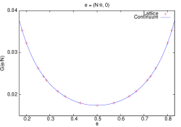
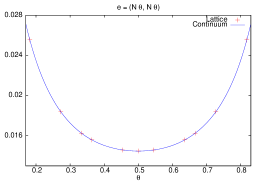
Figure 1: We show, for electric flux $\vec{e}=(N\theta,0)$ (left), and $\vec{e}=(N\theta,N\theta)$ (right), the function $G(\theta)$ that gives the one-loop correction to the energy of a one-gluon state, through Eq. (2.5). The blue line corresponds to Eq. (2.6), while the red points are derived using a lattice regularization in the calculation of the self-energy.

In perturbation theory the energy of electric flux can be determined by computing the gluon self-energy on the twisted box (for examples in SU(2) see Refs. [4, 5]). Details of the calculation at one-loop order will be presented elsewhere [6]. Here we simply provide the final expression that will be used to analyze the numerical results in section 3. Putting everything together, we obtain for the square of the energy of electric flux $\vec{e}$ with colour momentum $\vec{n}$:

$${E^{2}(\vec{e})\over\lambda^{2}}=\Big{(}{2\pi|\vec{n}|\over\lambda Nl}\Big{)}^{2}\,-\,{4\pi\over\lambda Nl}\,G\Big{(}{\vec{e}\over N}\Big{)}\quad,$$ (5)

where $\lambda=g^{2}N$ is the ’t Hooft coupling, which is dimensionful in 2+1 dimensions. The first order correction to the tree level expression is given in terms of:

$$G\Big{(}{\vec{e}\over N}\Big{)}=-{1\over 16\pi^{2}}\int_{0}^{\infty}{dx\over\sqrt{x}}\,\Big{(}\theta_{3}^{2}(0,ix)-\prod_{i=1}^{2}\,\theta_{3}({e_{i}\over N},ix)-{1\over x}\Big{)}$$ (6)

with the Jacobi Theta function given by:

$$\theta_{3}(z,ix)=\sum_{n\in{\bf Z}}\exp\{-x\pi n^{2}+2\pi inz\}\quad.$$ (7)

The dependence of $G$ on $\vec{e}/N$ is exhibited in Fig. 1, for electric fluxes of the form $\vec{e}=(N\theta,0)$ and $\vec{e}=(N\theta,N\theta)$.

One important remark at this stage is that, once $\vec{n}$ and $\vec{e}/N$ have been fixed, the energy depends exclusively on the variable $x=\lambda Nl$, which can be interpreted as the dimensionless ’t Hooft coupling corresponding to an effective box of size $Nl$. Based on our numerical results, we will argue that this is the case even in the non-perturbative regime. This will imply thus a kind of reduction in which $N$ and $l$ become interchangeable. A second remark in order is the non-analyticity of $G(\theta)$ at $\theta=0\,({\rm mod}\,1)$. This could give rise to a tachyonic instability in the energy of electric flux for $N\rightarrow\infty$, which has been previously discussed in the context of non-commutative geometry in Ref. [9]. There it was presented as an evidence of spontaneous $Z_{N}$ symmetry breaking. We will come back to this issue when discussing the numerical results in section 4.

Let us finally mention that in order to arrive at the one-loop perturbative expression we have used three different approaches: to compute the Euclidean gluon self-energy in the continuum and on the lattice, and to use the Hamiltonian formulation. The lattice calculation has made use of the results in Refs. [7],[8]. In Fig. 1, the lattice results for $G(\theta)$, extrapolated to the continuum limit, are compared with the formula given in Eq. (6). There is perfect agreement between the two.

3 Numerical Results

In this section we will present the results of a lattice calculation of the electric-flux spectrum in a twisted box as a function of $N$, $l$ and the magnetic flux. We start with a $L_{0}\times L^{2}$ lattice with twisted boundary conditions ($l=La$, with $a$ the lattice spacing). It is possible to perform a change of variables of the link matrices that allows to work with periodic links at the price of introducing a twist dependent factor in the action:

$$S_{W}=Nb\sum_{x}\sum_{\mu\neq\nu}\Big{(}N-z_{\mu\nu}^{*}(x)\,{\rm Tr}P_{\mu\nu}(x)\Big{)}\quad,$$ (8)

where $z_{\mu\nu}(x)=1$ except for the corner plaquettes in each (1,2) plane where it takes the value:

$$z_{ij}(x)=\exp\Big{\{}i\,{2\pi m\over N}\,\epsilon_{ij}\Big{\}}\quad,$$ (9)

with $m$ the magnetic flux. We have performed Monte Carlo simulations with this action employing a heat-bath algorithm based on a proposal by Fabricius and Haan [10]. Four sets of $(N,L,L_{0})$ values have been generated: (5,14,48), (5,22,72), (7,10,32), and (17,4,32), with values of the magnetic flux: $m=1,\,2$, for SU(5), $m=1,\,2,\,3$, for SU(7), and $m=1,\,3,\,5,\,8$, for SU(17).

The electric-flux spectrum has been extracted from spatially smeared Polyakov loop correlators. The spatial Polyakov loops, winding $e$ times around the $\hat{\imath}$th direction of the torus, read:

$$P_{i}(t,\,\vec{x},\,e)={\rm Tr}\Big{\{}\prod_{s=0}^{L-1}U_{i}\,(t,\,\vec{x}+s\hat{\imath})\Big{\}}^{e}\quad.$$ (10)

The twist gives rise to non-trivial boundary conditions for the loops: $P_{i}(t,\,\vec{x}+L\hat{\jmath},\,e)=z_{ij}^{\,e}\,\,P_{i}(t,\,\vec{x},\,e)$, that have to be considered when extracting the spectrum from the Polyakov loop correlators. In practice, we project over the different colour-momentum states by computing the averaged correlators:

$$C_{1}(t,\,e,\,n)={1\over L^{2}}\sum_{y,\tilde{y}=1}^{L}\exp\Big{\{}-i\,{2\pi n\over LN}\,\tilde{y}\Big{\}}\,\langle\,P_{1}(0,\,y\hat{\jmath},\,e)\,P_{1}^{\dagger}(t,\,(y+\tilde{y})\hat{\jmath},\,e)\,\rangle\quad,$$ (11)

with $e=\epsilon_{21}\,n\,\bar{k}$. An analogous expression holds for $C_{2}(t,\,e,\,n)$. The energy is extracted from the exponential decay at large $t$ of the correlator.

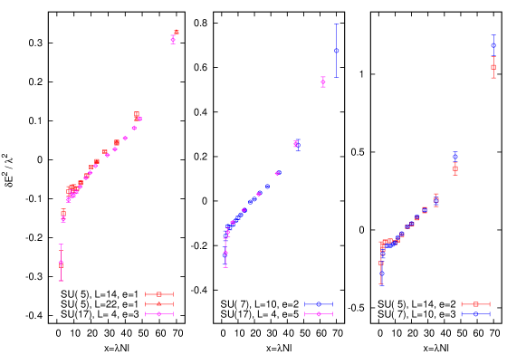
Figure 2: For different values of $l$, $N$, and $e$, we display the quantity $\delta E^{2}(e)/\lambda^{2}=(E^{2}-E_{0}^{2})/\lambda^{2}$ vs $x=\lambda Nl$, where $E$ is the energy of electrix flux $e$ with momentum $|\vec{n}|=1$, and $E_{0}=2\ {\rm asinh}(\sin(\pi/(NL)))$ is the lattice tree-level perturbative result.

A detailed account of the results will be presented in [6]. Here we will focus on a few examples that illustrate the scaling of the electric-flux energies with $x=\lambda Nl$. We will focus on the minimal momentum states with $|\vec{n}|=1$ which have electric flux $|\vec{e}|=\bar{k}$. According to our perturbative calculation, for given $e/N$ we expect energies to depend solely on $x$. Given that $N$ is prime, identical ratios of $e/N$ are not possible, nevertheless our data falls in three sets with similar values for the ratio: $(N,e)=\{(5,1),(17,3)\};\,\{(7,2),(17,5)\};\,\{(5,2),(7,3)\}$. The dependence of the energy squared on $x$ is presented in Fig. 2. The scaling holds in all the range of $x$ analyzed which goes far beyond the perturbative regime. A discussion of the results will be presented below.

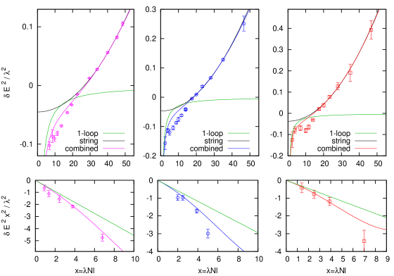
Figure 3: In the upper panels we display several fits of $\delta E^{2}(e)/\lambda^{2}$ to Eq. (4.4). The symbol codes are the same as in Fig. 2. Different lines correspond to: (combined) $\alpha=G(e/N)$, $\beta$ and $\gamma$ free; (1-loop) $\alpha=G(e/N)$, $\beta=\gamma=0$; (string) $\alpha=0$, $\beta$ and $\gamma$ free. The lower panels display $\delta E^{2}(e)x^{2}/\lambda^{2}$.

4 Discussion

Our numerical results indicate that the energy of electric flux, in units of the ’t Hooft coupling, depends solely on the variable $x=\lambda Nl$ and the value of $e/N$, at least for the minimal momentum $|\vec{n}|=1$. This does indeed hold for the perturbative expression. Let us look now at the expectation in the large $x$ regime, where strings of electric flux are expected to be formed and the energy should grow linearly with the box size $l$. A large amount of lattice results hint in the direction that flux tubes can be described in terms of an effective string picture based on the Nambu-Goto action [3]. In the presence of a constant background magnetic field $B$, the Nambu-Goto prediction for a closed-string winding $\vec{e}$ times around the torus is given by:

$${E^{2}(\vec{e})\over\lambda^{2}}=\Big{(}{\sigma|\vec{e}|\over\lambda^{2}N}\Big{)}^{2}(\lambda Nl)^{2}-{\pi\sigma\over 3\lambda^{2}}+\sum_{i}\Big{(}{\epsilon_{ij}e_{j}\,B\over\lambda l}\Big{)}^{2}\quad,$$ (12)

where $\sigma$ is the fundamental string tension. The last term on the right hand side of this formula can be easily mapped onto the tree-level perturbative expression $E_{0}^{2}$ by taking into account the relation between $\vec{n}$ and $\vec{e}$, and identifying the magnetic field with $B=2\pi m/N$. If the Nambu-Goto expression would hold, two different regimes would take place in terms of the scaling variable $x$:

• Low $x$, where:

  $${E^{2}(\vec{e})\over\lambda^{2}}-{E_{0}^{2}(\vec{e})\over\lambda^{2}}=-\,{4\pi\over x}\,G\Big{(}{\vec{e}\over N}\Big{)}\quad.$$ (13)

• Large $x$, where:

  $${E^{2}(\vec{e})\over\lambda^{2}}-{E_{0}^{2}(\vec{e})\over\lambda^{2}}=\Big{(}{\sigma|\vec{e}|\over\lambda^{2}N}\Big{)}^{2}x^{2}-{\pi\sigma\over 3\lambda^{2}}\quad.$$ (14)

This would be fully consistent with our hypothesis on the $x$ scaling, once $\vec{e}/N$ is fixed. A formula that captures the asymptotic behaviour in both the low and large $x$ regimes is:

$${\delta E^{2}(e)\over\lambda^{2}}={E^{2}(e)\over\lambda^{2}}-{E_{0}^{2}(e)\over\lambda^{2}}=-{4\pi\alpha\over x}-{\pi\beta\over 3}+\gamma^{2}\,x^{2}\quad.$$ (15)

Fitting this expression to our data gives the results displayed in Fig. 3. The fits are restricted to the large $x$ region with $x>20$ ($x>30$, for $N=17$, $e=3$). Two different fits are presented: (a) fixing $\alpha=G(e/N)$, denoted by ‘combined’, and (b) fixing $\alpha=0$, denoted by ‘string’. In all cases, the ‘combined’ fit has a slightly better $\chi^{2}$ per degree of freedom than the ‘string’ fit. In addition, we display the 1-loop expression. Although the combined formula fails to reproduce the results in the intermediate $x$ region it describes qualitatively quite well the data. One remarkable observation is that for small $x$ it improves the one-loop result in the correct direction. This is clearly observed in the low panels of Fig. 3 where $\delta E^{2}x^{2}/\lambda^{2}$ is plotted to enhance this effect. We are at present exploring alternative parametrizations to improve the fit in the intermediate $x$ regime.

One final remark refers to the possible existence of tachyonic instabilities. One could use Eq. (15) to see in which instances the energy remains non-tachyonic for all values of $x$. A more thorough analysis will be presented in [6]. Let us just mention here that our results indicate that it suffices to keep both $m$ and $\bar{k}$ of order $N$ to avoid the tachyonic behaviour. This coincides with the criteria introduced in [2] for twisted Eguchi-Kawai reduction to hold at large $N$.

- [1] T. Eguchi and H. Kawai, Phys. Rev. Lett. 48, 1063 (1982).
- [2] A. González-Arroyo and M. Okawa, JHEP 1007, 043 (2010); The string tension from smeared Wilson loops at large N, arXiv:1206.0049 [hep-th]; PoS(Lattice 2012)221.
- [3] R. Narayanan and H. Neuberger, PoS LAT 2007 (2007) 020. M. Teper, Acta Phys. Polon. B 40 (2009) 3249. B. Lucini and M. Panero, SU(N) gauge theories at large N, arXiv:1210.4997 [hep-th].
- [4] A. González Arroyo and C. P. Korthals Altes, Nucl. Phys. B 311 (1988) 433.
- [5] D. Daniel, A. González-Arroyo, C. P. Korthals Altes and B. Soderberg, Phys. Lett. B 221 (1989) 136; D. Daniel, A. González-Arroyo and C. P. Korthals Altes, Phys. Lett. B 251, 559 (1990).
- [6] M. García Perez, A. González Arroyo and M. Okawa, Small volume Physics in the 2+1 dimensional Yang-Mills theory, to appear.
- [7] J. R. Snippe, Phys. Lett. B 389, 119 (1996); Nucl. Phys. B 498, 347 (1997).
- [8] M. Luscher and P. Weisz, [Erratum-ibid. 98 (1985) 433]; Phys. Lett. B 158 (1985) 250; Nucl. Phys. B 266 (1986) 309.
- [9] Z. Guralnik, R. C. Helling, K. Landsteiner and E. López, JHEP 0205, 025 (2002).
- [10] K. Fabricius and O. Haan, Phys. Lett. B 143 (1984) 459.