Current Status of Indirect CP Violation in Neutral Kaon System

Abstract:

In the standard model (SM), the CP violation is introduced through a single phase in the CKM matrix. The neutral kaon system is one of the most precise channels to test how the SM theory describes the experiment data such as $\epsilon_{K}$ accurately. The indirect CP violation is parametrized into $\epsilon_{K}$, which can be calculated directly using lattice QCD. In this calculation, the largest uncertainty comes from two sources: one is $\hat{B}_{K}$ and the other is $V_{cb}$. We use the lattice results of $\hat{B}_{K}$ and exclusive $V_{cb}$ to calculate the theoretical estimate of $\epsilon_{K}$, which turns out to be $3.1\sigma$ away from its experimental value. Here, the error is evaluated using the standard error propagation method.

1stRGB255,165,0 2ndRGB135,206,250 3rdRGB173,255,47

1 Introduction

The neutral kaon system has two kinds of CP violation: indirect and direct CP violation. Indirect CP violation is parametrized into $\epsilon_{K}$. The experimental value of $\epsilon_{K}$ is very well known [1]:

$$\epsilon_{K} =(2.228\pm 0.011)\times 10^{-3}\times e^{i\phi_{\epsilon}}\,,\qquad\phi_{\epsilon}=43.51\pm 0.05.$$ (1)

We can also calculate $\epsilon_{K}$ directly from the SM using $B_{K}$, $V_{cb}$, and other input parameters, which are determined from other experiments and the SM theory. By comparing these two values, we can test a fundamental ansatz of the SM, the unitarity of the CKM matrix.

Here, we calculate $\epsilon_{K}$ directly from the SM using the known parameters with their errors in control. Two of the most important input parameters are $\hat{B}_{K}$ and $V_{cb}$, which dominate the statistical and systematic uncertainty in $\epsilon_{K}$. During a past decade, lattice QCD has reduced the $B_{K}$ error dramatically down to less than 5% level [2, 3, 4] as well as $V_{cb}$ [5].

There are two independent methods to determine $V_{cb}$: inclusive channels and exclusive channel. There exists about $2~{}3\sigma$ difference in $V_{cb}$ between inclusive and exclusive methods. We address this issue on how this have an effect on $\epsilon_{K}$.

Here, we use the Wolfenstein parameters for the CKM matrix to calculate $\epsilon_{K}$ mainly because they are convenient.

Let us define a parameter $\Delta$ which test the unitarity ansatz directly as

$$\Delta\equiv V\cdot V^{\dagger}-I.$$

Here, we calculate $\epsilon_{K}$ and $\Delta$ to test the SM. The CKM matrix elements are accurate up to $\mathcal{O}(\lambda^{5})\approx 3\times 10^{-4}$. We use the standard error propagation method to estimate the errors.

2 Review of the Neutral Kaon Mixing: $\epsilon_{K}$

The neutral kaon system forms a two dimensional Hilbert space. In this subspace, the time evolution of the neutral kaon state vectors can be described by the effective Hamiltonian $\hat{H}_{\text{eff}}$

$$i\frac{d}{dt}\lvert K(t)\rangle=\hat{H}_{\text{eff}}\lvert K(t)\rangle,\quad\hat{H}_{\text{eff}}=\hat{M}-i\frac{\hat{\Gamma}}{2}.$$ (2)

$\hat{M}$ $(\hat{\Gamma})$ is the dispersive (absorptive) part. Here, the dispersive part gives the mass eigenvalues of $K_{S}$ and $K_{L}$, and the absorptive part represents the decay rates of $K_{S}$ and $K_{L}$. Let us take the basis with the CP even $\lvert K_{1}\rangle$ and odd $\lvert K_{2}\rangle$ states,

$$\lvert K_{1}\rangle=\frac{1}{\sqrt{2}}\big{(}\lvert K^{0}\rangle+\lvert\overline{K}^{0}\rangle\big{)},\quad\lvert K_{2}\rangle=\frac{1}{\sqrt{2}}\big{(}\lvert K^{0}\rangle-\lvert\overline{K}^{0}\rangle\big{)}.$$ (3)

In this basis, the matrix elements can be written as the followings:

$$M=\begin{pmatrix}M_{1}&+im^{\prime}\\ -im^{\prime}&M_{2}\end{pmatrix},\;\Gamma=\begin{pmatrix}\Gamma_{1}&+i\gamma^{\prime}\\ -i\gamma^{\prime}&\Gamma_{2}\end{pmatrix}.$$ (4)

By construction of the formal perturbation theory in quantum field theory known as the Wigner-Weisskopf theory [6], $M$ and $\Gamma$ are hermitian matrices. In addition, if we assume that the CPT invariance is exactly respected, then $m^{\prime}$ and $\gamma^{\prime}$ must be real.

Solving the eigenvalue problem with this matrix representation for $H_{\text{eff}}$, the eigenstates

$$\lvert K_{S}\rangle=\frac{1}{\sqrt{1+\lvert\tilde{\epsilon}\rvert^{2}}}(\lvert K_{1}\rangle+\tilde{\epsilon}\lvert K_{2}\rangle),\quad\lvert K_{L}\rangle=\frac{1}{\sqrt{1+\lvert\tilde{\epsilon}\rvert^{2}}}(\lvert K_{2}\rangle+\tilde{\epsilon}\lvert K_{1}\rangle)$$ (5)

have the mass $M_{S,L}$ and the decay rate $\Gamma_{S,L}$, respectively. The small CP impurity $\tilde{\epsilon}$ satisfies the following equation

$$\tilde{\epsilon}=\tilde{\epsilon}_{(0)}(1+\tilde{\epsilon}^{2}).$$ (6)

Here, the $\tilde{\epsilon}_{(0)}$ parameter is defined as

$$\tilde{\epsilon}_{(0)}\equiv\frac{-i\big{(}m^{\prime}-\frac{i}{2}\gamma^{\prime}\big{)}}{\big{(}M_{1}-M_{2}\big{)}-\frac{i}{2}\big{(}\Gamma_{1}-\Gamma_{2}\big{)}}=e^{i\theta}\sin{\theta}(\frac{m^{\prime}}{\Delta M_{K}}-i\cot{\theta}\frac{\gamma^{\prime}}{\Delta\Gamma_{K}})+\mathcal{O}\big{(}{\tilde{\epsilon}_{(0)}}^{3}\big{)},$$ (7)

where

$$\Delta M_{K}=M_{L}-M_{S},\;\Delta\Gamma_{K}=\Gamma_{S}-\Gamma_{L},\;\tan{\theta}=\frac{2\Delta M_{K}}{\Delta\Gamma_{K}}.$$ (8)

The solution of $\tilde{\epsilon}$ can be obtained by iteration. Since $\tilde{\epsilon}_{(0)}$ is of the order of $10^{-3}$, we may expand $\tilde{\epsilon}$ perturbatively as follows,

$$\tilde{\epsilon}=\tilde{\epsilon}_{(0)}+{\tilde{\epsilon}_{(0)}}^{3}+2{\tilde{\epsilon}_{(0)}}^{5}+5{\tilde{\epsilon}_{(0)}}^{7}+\cdots.$$ (9)

In Eq. (7), $M_{1,2}$ and $\Gamma_{1,2}$ can be safely replaced by the eigenvalues $M_{S,L}$ and $\Gamma_{S,L}$ which are experimental observables. Note that this approximation makes an error of the size $\mathcal{O}({\tilde{\epsilon}_{(0)}}^{3})\approx 10^{-9}$ which is of no interest to us. In the case of $\gamma^{\prime}/\Delta\Gamma_{K}$, we presume the following assumptions:

• First, we make the approximation $\Delta\Gamma_{K}\cong\Gamma_{1}$ which is good up to the precision of $10^{-3}$.

• Second, we assume that the contribution from the two pion state is dominant in $\gamma^{\prime},\Gamma_{1}$ which is good in the precision level of $10^{-3}$.

• Third, we assume that the contribution from the $I=0$ two pion state is dominant in $\gamma^{\prime},\Gamma_{1}$ compared with that from the $I=2$ state. This approximation is good up to the precision of $10^{-7}$.

Using these assumptions, we can approximate the $\gamma^{\prime}/\Delta\Gamma_{K}$ as follows,

$$\frac{\gamma^{\prime}}{\Delta\Gamma_{K}}=\xi_{0}+\mathcal{O}\big{(}10^{-7}\big{)},\quad\xi_{0}\equiv\frac{\mathrm{Im}A_{0}}{\mathrm{Re}A_{0}}.$$ (10)

Then, we can express $\epsilon_{K}$ approximately as follows,

$$\epsilon_{K} \equiv\frac{\langle\pi\pi(I=0)\lvert H_{W}\rvert K_{L}\rangle}{\langle\pi\pi(I=0)\lvert H_{W}\rvert K_{S}\rangle}=\tilde{\epsilon}_{(0)}+i\xi_{0}+\mathcal{O}\big{(}{\tilde{\epsilon}_{(0)}}^{3}\big{)}=e^{i\theta}\sin{\theta}\Big{(}\frac{m^{\prime}_{(6)}}{\Delta M_{K}}+\xi_{0}\Big{)}+\Delta\epsilon_{K}\,.$$ (11)

The correction of $\mathcal{O}({\tilde{\epsilon}_{(0)}}^{3})$ in Eq. (11) is smaller than both the current experiment precision and the size of the long distance contributions of the $m^{\prime}$ [7]. The last expression in Eq. (11) is obtained by substituting $\tilde{\epsilon}_{(0)}$ with Eq. (7) and Eq. (10). The correction of $\Delta\epsilon_{K}$ contains both short-distance (SD) contribution and long-distance (LD) contribution, which are expected to be about $\approx 5\%$[7]. Here, we also neglect this contribution from $\Delta\epsilon_{K}$, mainly because it is not known to a sufficient precision theoretically.

In this analysis, we take into account only the short-distance contribution from the dimension 6 operators $m^{\prime}_{(6)}$. In the SM, this part can be calculated from the box diagram [8]. Here, we follow the notations in [8]. Then, we can obtain the following master formula which will be used in this analysis:

$$\lvert\epsilon_{K}^{\text{SM}}\rvert=\sqrt{2}\sin{\theta}\Big{(}C_{\epsilon}\hat{B}_{K}X+\xi_{0}\Big{)},$$ (12)

where

$$X =\bar{\eta}\lambda^{2}\lvert V_{cb}\rvert^{2}\times\Big{[}\lvert V_{cb}\rvert^{2}(1-\bar{\rho})\eta_{2}S_{0}(x_{t})+\eta_{3}S_{0}(x_{c},x_{t})-\eta_{1}S_{0}(x_{c})\Big{]}$$ (13)

$$C_{\epsilon} =\frac{G_{F}^{2}F_{K}^{2}m_{K^{0}}M_{W}^{2}}{6\sqrt{2}\pi^{2}\Delta M_{K}}.$$ (14)

where we use the experimental value for $\Delta M_{K}$. The input $\xi_{0}$ has been taken from the lattice calculation which accounts the long distance contribution.

$G_{F}$	$1.16637(1)\times 10^{-5}$ GeV-2	[1]
$M_{W}$	80.399(23) GeV	[1]
$m_{c}(m_{c})$	$1.25(9)$ GeV	[10]
$m_{t}(m_{t})$	$162.7(1.3)$ GeV	[10]
$\eta_{1}$	$1.43(23)$	[10]
$\eta_{2}$	$0.5765(65)$	[10]
$\eta_{3}$	$0.47(4)$	[10]
$\theta$	$43.51(5)^{\circ}$	[1]
$m_{K^{0}}$	$497.614(24)$ MeV	[1]
$\Delta M_{K}$	$3.483(6)\times 10^{-12}$ MeV	[1]

(a)

$A$	$0.808(22)$	[1] CKMfitter
	$0.832(17)$	[1] UTfit
$\lambda$	$0.2253(7)$	[1] CKMfitter
	$0.2246(11)$	[1] UTfit
$\bar{\rho}$	$\displaystyle 0.132^{+0.022}_{-0.014}$	[1] CKMfitter
	$0.130(18)$	[1] UTfit
$\bar{\eta}$	$0.341(13)$	[1] CKMfitter
	$0.350(13)$	[1] UTfit

(b) Wolfenstein Parameters

$F_{K}$	$156.1(0.2)(0.8)(0.2)$ MeV	[1]
	$156.1(1.1)$ MeV	[11] LAT.AVG.
$\hat{B}_{K}$	$0.7674(99)$	[11] LAT.AVG.
	$0.727(4)(38)$	[2] SWME
$\xi_{0}$	$-1.63(19)(20)\times 10^{-4}$	[13]

(c) Lattice Calculation

$\lvert V_{cb}\rvert$	$41.85(42)(9)(59)\times 10^{-3}$	[12] $(X_{c}l\nu+X_{s}\gamma)_{\text{Kin}}$
	$41.68(44)(9)(58)\times 10^{-3}$	[12] $(X_{c}l\nu)_{\text{Kin}}$
	$41.87(25)\times 10^{-3}$	[12] $(X_{c}l\nu+X_{s}\gamma)_{\text{1S}}$
	$42.31(36)\times 10^{-3}$	[12] $(X_{c}l\nu)_{\text{1S}}$
	$41.5(7)\times 10^{-3}$	[1] Incl.PDG.AVG.
	$39.5(1.0)\times 10^{-3}$	[11] Excl.

(d) $V_{cb}$

Table 1: Input Parameters

3 Input Parameters

The parameters, $m_{c},m_{t},\eta_{1},\eta_{2},\eta_{3}$ depend on the renormalization scheme, and so are taken from the single reference for consistency (Table 1a). The CKMfitter and UTfit results in Table 1b are obtained by their own global fit method using the same PDG inputs.

In $\hat{B}_{K}$ calculation in Table 1c, BMW quotes the smallest systematic error. It dominates the smallness of the lattice average error. RBC-UKQCD collaboration calculates $\mathrm{Im}A_{2}$ on the lattice. Using this value, they determine $\xi_{0}$ through the relation

$$\mathrm{Re}\Big{(}\frac{\epsilon^{\prime}_{K}}{\epsilon_{K}}\Big{)}=\frac{1}{\sqrt{2}\lvert\epsilon_{K}\rvert}\frac{\mathrm{Re}A_{2}}{\mathrm{Re}A_{0}}\Big{(}\frac{\mathrm{Im}A_{2}}{\mathrm{Re}A_{2}}-\xi_{0}\Big{)}.$$ (15)

Other inputs such as $\mathrm{Re}A_{0},\mathrm{Re}A_{2},\epsilon_{K},$ and ${\epsilon^{\prime}_{K}}/{\epsilon_{K}}$ are taken from experiments.

Inclusive $V_{cb}$ can be extracted from global fit of measured moments (lepton energy, hadronic mass, and photon energy) of the decay channels:

$$B\rightarrow X_{c}l\nu,\;\qquad B\rightarrow X_{s}\gamma.$$

We use the PDG average value as the representative of the inclusive $V_{cb}$. The quoted exclusive $V_{cb}$ is the average of two semi-leptonic decay channels:

$$B\rightarrow D^{*}\ell\nu\,,\qquad B\rightarrow D\ell\nu\,.$$

For each scalar and vector channel, HFAG result is combined with FNAL/MILC lattice QCD calculation of the zero recoil form factor.

4 Error Estimate

For the function with $N$ arguments, the error propagation formula gives the combined error $\sigma_{f}$ in terms of the errors of each arguments:

$$\sigma_{f}^{2}=\sum_{j,k=1}^{N}C_{jk}\frac{\partial f(\mathbf{x})}{\partial x_{j}}\bigg{|}_{\langle\mathbf{x}\rangle}\frac{\partial f(\mathbf{x})}{\partial x_{k}}\bigg{|}_{\langle\mathbf{x}\rangle}\sigma_{x_{j}}\sigma_{x_{k}},$$ (16)

where $C_{jk}$ denotes the normalized correlation between the parameters $x_{j}$ and $x_{k}$, and $|C_{ij}|\leq 1$. Especially the diagonal components $C_{ii}=1$. We turn off the correlation and so $C_{ij}=\delta_{ij}$. In the case of asymmetric error, $\bar{\rho}$ given by CKMfitter, we take a larger error and treat it as a symmetric error.

For $\epsilon_{K}^{\text{SM}}$,

$$f(\mathbf{x}) =\lvert\epsilon_{K}(\mathbf{x})\rvert$$ (17)

$$\mathbf{x} =(\theta,G_{F},F_{K},m_{K^{0}},M_{W},\Delta M_{K},\xi_{0},\hat{B}_{K},\lambda,\bar{\rho},\bar{\eta},\lvert V_{cb}\rvert,\eta_{1},\eta_{2},\eta_{3},x_{c},x_{t}).$$ (18)

To check the unitarity of the CKM matrix,

$$f_{ij}(\mathbf{x}) =[V(\mathbf{x})V^{{\dagger}}(\mathbf{x})-I]_{ij}\equiv\Delta_{ij}$$ (19)

$$\mathbf{x} =(A,\lambda,\rho,\eta;\lvert V_{cb}\rvert).$$ (20)

We use the Wolfenstein parametrization to evaluate each elements of the CKM matrix $V_{ij}$, except for $V_{cb}$ itself. Real and imaginary part of $\Delta_{ij}$ are separately treated.

5 Results

The Wolfenstein parameter set, $\hat{B}_{K}$, and $V_{cb}$ has a multiple choice. It forms 8 input parameter sets. We calculate $\epsilon_{K}^{\text{SM}}$ for these sets as shown in Fig. 1. We find out that $\lvert\epsilon_{K}\rvert$ shows $3.1\sigma$ tension between $\lvert\epsilon_{K}^{\text{Exp}}\rvert$ and $\lvert\epsilon_{K}^{\text{SM}}\rvert$, using exclusive $V_{cb}$ and SWME calculation of $B_{K}$ as shown in Fig. 1a. With the UTfit Wolfenstein parameters, the tension is slightly reduced to $2.9\sigma$ [Fig. 1b].

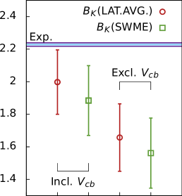
(a) CKMfitter

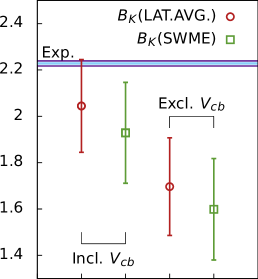
(b) UTfit

Figure 1: $\epsilon_{K}(\times 10^{3})$

The deviation matrix $\Delta$ provides a test of the Wolfenstein parameters, outputs of the global fit. These are inputs for the $\epsilon_{K}^{\text{SM}}$, as well. So testing the compatibility between the global fit results and the $V_{cb}$ is needed to interpret the difference between $\epsilon_{K}^{\text{SM}}$ and $\epsilon_{K}^{\text{SM}}$. We find that the numerical size of $\Delta_{ij}$ has the following hierarchy

$$10^{2}\mathcal{O}\big{(}\lvert\mathrm{Re}\Delta_{12}\rvert\big{)}=10\mathcal{O}\big{(}\lvert\mathrm{Re}\Delta_{22}\rvert\big{)}=\mathcal{O}\big{(}\lvert\mathrm{Re}\Delta_{23}\rvert\big{)}\,.$$ (21)

$\mathrm{Re}\Delta_{22}$ shows that the difference between exclusive $V_{cb}$ and Wolfenstein parameters from CKMfitter (UTfit) are about $1.0\sigma$ ($1.8\sigma$) as shown in Fig. 2a and 2b. $\mathrm{Re}\Delta_{23}$ shows the difference about $1.0\sigma$ ($1.8\sigma$) as shown in Fig. 2c and 2d. Other components of $\Delta$, which does not depend on the choice of inclusive or exclusive $V_{cb}$, are so small as to be consistent with the unitary ansatz.

In Table 2, $V_{cb}$ dominates the error of $\epsilon_{K}^{\text{SM}}$ regardless of the inclusive or exclusive determination. In case of the SWME calculation of $B_{K}$ and inclusive $V_{cb}$, both contribute to the total error in comparable size. In the case of the lattice average of $B_{K}$, $V_{cb}$ becomes an extremely dominant error and the subdominant error comes from $\bar{\eta}$.

W.P.	$V_{cb}$	$B_{K}$	$m_{c}$	$\eta_{1}$	$\eta_{3}$	$F_{K}$	$B_{K}$	$\xi_{0}$	$\bar{\rho}$	$\bar{\eta}$	$V_{cb}$
CKMfitter	Incl.	LAT.AVG.	$10.62$	$5.24$	3rd$12.50$	$2.36$	$1.98$	$1.85$	$4.29$	2nd$17.29$	1st$41.43$
		SWME	$8.10$	$4.00$	$9.53$	$1.80$	2nd$25.06$	$1.57$	$3.28$	3rd$13.19$	1st$31.61$
	Excl.	LAT.AVG.	$7.94$	$3.92$	3rd$9.34$	$1.53$	$1.28$	$1.68$	$2.63$	2nd$11.17$	1st$58.99$
		SWME	$6.61$	$3.26$	$7.78$	$1.27$	2nd$17.67$	$1.56$	$2.19$	3rd$9.29$	1st$49.10$

Table 2: Error Fractions $\sigma_{i}^{2}/\sum\sigma_{j}^{2}$. The UTfit Wolfenstein parameters(W.P) show the same tendency.

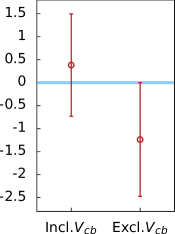
(a) $\mathrm{Re}\Delta_{22}$(CKMfitter)

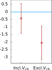
(b) $\mathrm{Re}\Delta_{22}$(UTfit)

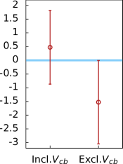
(c) $\mathrm{Re}\Delta_{23}$(CKMfitter)

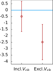
(d) $\mathrm{Re}\Delta_{23}$(UTfit)

Figure 2: $\mathrm{Re}\Delta_{22}(\times 10^{4})$ and $\mathrm{Re}\Delta_{23}(\times 10^{3})$ to test the CKM unitarity.

6 Acknowledgements

The research of W. Lee is supported by the Creative Research Initiatives Program (2012-0000241) of the NRF grant funded by the Korean government (MEST). W. Lee would like to acknowledge the support from KISTI supercomputing center through the strategic support program for the supercomputing application research [No. KSC-2011-G2-06]. Computations were carried out in part on QCDOC computing facilities of the USQCD Collaboration at Brookhaven National Lab, on GPU computing facilities at Jefferson Lab, on the DAVID GPU clusters at Seoul National University, and on the KISTI supercomputers. The USQCD Collaboration are funded by the Office of Science of the U.S. Department of Energy.

References

- [1] K. Nakamura et. al. (Particle Data Group), J.Phys.G G37 (2010) 075021.
- [2] T. Bae et. al., Phys.Rev.Lett. 109 (2012) 041601 [hep-lat/1111.5698].
- [3] Y. Aoki et. al., Phys. Rev. D84 (2011) 014503 [hep-lat/1012.4178].
- [4] C. Aubin et. al., Phys. Rev. D81 (2010) 014507 [hep-lat/0905.3947].
- [5] J. Bailey et. al., \posPoS(LATTICE2010)311 [hep-lat/1011.2166].
- [6] N. Christ, in Proceedings of Lattice2011 \posPoS(LATTICE2011)277 [hep-lat/1201.2065].
- [7] A. J. Buras, D. Guadagnoli and G. Isidori, Phys. Lett. B688 (2010) 309 [hep-ph/1002.3612].
- [8] A. J. Buras, Weak Hamiltonian, CP violation and rare decays in Probing the Standard Model of Particle Interactions, F. David and R. Gupta, eds., Elsevier Science B.V. (1998) [hep-ph/9806471].
- [9] J. Brod and M. Gorbahn, Phys.Rev.Lett 108 (2012) 121801 [hep-ph/1108.2036].
- [10] A. J. Buras, and D. Guadagnoli, Phys.Rev. D78 (2008) 033005 [hep-ph/0805.3887].
- [11] J. Laiho, and E. Lunghi, and R. S. Van de Water, Phys.Rev. D81 (2010) 034503 [hep-ph/0910.2928] http://latticeaverages.org/.
- [12] J. Laiho, and B. D. Pecjak, and C. Schwanda, in Proceedings of CKM2010 (2011) [hep-ex/1107.3934].
- [13] T. Blum et. al., Phys.Rev.Lett. 108 (2012) 141601 [hep-lat/1111.1699].