The Shakura-Sunyaev viscosity prescription with variable $\alpha(r)$

Abstract

Almost all hydrodynamic accretion disk models parametrize viscosity with the dimensionless parameter $\alpha$. There is no detailed model for $\alpha$, so it is usually taken to be a constant. However, global simulations of magnetohydrodynamic disks find that $\alpha$ varies with distance from the central object. Also, Newtonian simulations tend to find smaller $\alpha$’s than general relativistic simulations. We seek a one-dimensional model for $\alpha$ that can reproduce these two observations. We are guided by data from six general relativistic magnetohydrodynamic accretion disk simulations. The variation of $\alpha$ in the inner, laminar regions of the flow results from stretching of mean magnetic field lines by the flow. The variation of $\alpha$ in the outer, turbulent regions results from the dependence of the magnetorotational instability on the dimensionless shear rate. We give a one-dimensional prescription for $\alpha(r)$ that captures these two effects and reproduces the radial variation of $\alpha$ observed in the simulations. For thin disks, the prescription simplifies to the formula $\alpha(r)=0.025\left[q(r)/1.5\right]^{6}$, where the shear parameter, $q(r)$, is an analytical function of radius in the Kerr metric. The coefficient and exponent are inferred from our simulations and will change as better simulation data becomes available. We conclude that the $\alpha$-viscosity prescription can be extended to the radially varying $\alpha$’s observed in simulations. It is possible that Newtonian simulations find smaller $\alpha$’s than general relativistic simulations because the shear parameter is lower in Newtonian flows.

1 Introduction

Accretion disk magnetic fields and turbulence act as a large scale viscosity, draining angular momentum and energy from accreting gas. The magnitude of this viscosity is uncertain, which adds a free parameter to accretion disk models. For example, Pringle & Rees (1972) leave the ratio of the disk’s radial velocity to its circular velocity as a free parameter. They call this ratio $y/100$ and estimate $y\sim 1$. They note that $y$ might be radius dependent and that a strong radial dependence could change qualitative features of the disk. However, other important features of the disk, such as its luminosity, depend weakly or not at all on $y$, so progress is possible without a detailed model for $y$.

Shakura & Sunyaev (1973) parametrized the viscosity with $\alpha$, the ratio of stress to pressure. It is related to Pringle and Rees’s $y$ by $y=100\alpha(h/r)^{2}$, where $h/r$ is the disk opening angle. They anticipated that $\alpha$ will be a function of radius, citing experiments of turbulence in Taylor-Coutte flow, flow between rotating cylinders (Taylor, 1936). These experiments show that the torque exerted by a turbulent flow on the cylinders depends on the rotation rate of the cylinders and the separation between them. The torque in the experiment is related to $\alpha$, so $\alpha$ should depend on accretion flow properties that vary with radius. The analogy is too rough to produce a quantitative model, so they assume $\alpha$ is a constant for simplicity.

The most significant theoretical breakthrough towards an understanding of $\alpha$ has been the realization that the magnetorotational instability (MRI) can drive turbulence in ionized accretion disks (Velikhov, 1959; Chandrasekhar, 1960; Balbus & Hawley, 1991, 1998). A weak seed magnetic field and a radially decreasing angular velocity profile are all that are required to trigger the instability and both are present in disks. This makes it possible to run magnetohydrodynamic (MHD) disk simulations without using the $\alpha$-viscosity prescription.

Nonetheless, because of its relative simplicity, the $\alpha$-viscosity prescription has not dimmed in importance. Over the past year, more than 300 papers cited the pioneering work of Shakura & Sunyaev (1973) and more than 1000 papers made reference to some disk solution based on the $\alpha$-viscosity prescription (such as the relativistic thin disk of Novikov & Thorne (1973) or the advection dominated accretion flow (ADAF) of Narayan & Yi (1994)). However, despite its interest, there is still no widely accepted model for the size or shape of $\alpha$. In applications, it is typically assumed to be a constant between 0.01 and 0.1 (e.g., Gou et al., 2011).

There are two varieties of MHD simulations, local and global, and both provide hints about the size and shape of $\alpha$. A standard setup for a local simulation is a box of weakly magnetized fluid in the shearing sheet approximation (e.g., Hawley & Balbus, 1991; Brandenburg et al., 1995; Hawley et al., 1995, 1996; Stone & Balbus, 1996; Brandenburg, 2001; Sano et al., 2004). The dimensions of the box are typically a few disk scale heights. The earliest global simulations of MRI turbulent disks used a Newtonian potential (Armitage, 1998; Matsumoto, 1999; Hawley, 2000; Machida et al., 2000) and, later, a pseudo-Newtonian potential (Hawley & Krolik, 2001). The first general relativistic global simulations were carried out by De Villiers et al. (2003). A standard setup for global simulations is a torus of fluid in hydrostatic equilibrium, threaded with a weak magnetic field (e.g., De Villiers et al., 2003). In local and global simulations, differential rotation triggers the MRI and drives turbulence. When the simulation reaches a quasi-steady state, one can compute the ratio of stress to pressure and so measure $\alpha$. Local simulations focus on resolving small scale physics, such as saturation of the MRI, while global simulations attempt a complete portrait of the accretion disk.

Global simulations have hinted at the shape of $\alpha$. Penna et al. (2010) and Penna et al. (2012b) presented general relativistic MHD (GRMHD) simulations of MRI turbulent disks in the Kerr metric, the spacetime of a spinning black hole. They confirmed that the relativistic $\alpha$-disk model of Novikov & Thorne (1973) gives a good description of the simulation data. This was partly motivated by earlier suggestions that magnetic stresses at the inner edges of MHD disks invalidate the assumptions of $\alpha$-disk models (e.g., Krolik, 1999; Agol & Krolik, 2000). The GRMHD simulations produced luminosity inside the innermost stable circular orbit (ISCO), where the Novikov & Thorne (1973) model is entirely dark, but it was a modest contribution to the total luminosity of the disk (on the order of a few percent; Kulkarni et al., 2011). Later, Penna et al. (2012b) generalized the Novikov & Thorne (1973) model to self-consistently incorporate nonzero luminosity inside the ISCO, bringing it closer to the GRMHD simulations.

Penna et al. (2010) and Penna et al. (2012b) measured the shape of $\alpha$. For accretion onto a non-spinning black hole, they found $\alpha$ is small at the event horizon, increases to a maximum near the photon orbit, declines to $\sim 0.06$ near the ISCO, and then continues to decline, albeit more slowly (see, e.g., Figure 7 of Penna et al., 2012b). In a completely different context, MHD simulations of protoplanetary disks, Fromang et al. (2011) found a radially varying $\alpha$ with similar shape. However, the overall size of their $\alpha$ was over an order of magnitude lower, peaking at 0.013 and declining to below 0.002.

The value of $\alpha$ is notoriously difficult to pin down (Pessah et al., 2007). Local simulations find that $\alpha$ is strongly affected by grid scale dissipation as well as stratification (Lesur & Longaretti, 2007; Fromang & Papaloizou, 2007; Simon & Hawley, 2009; Davis et al., 2010). In global and local simulations, $\alpha$ depends non-monotonically on resolution at all but the highest resolutions (Sorathia et al., 2012). In models with net magnetic flux, $\alpha$ scales with increasing flux (Hawley et al., 1995; Sano et al., 2004; Pessah et al., 2007). Finally, $\alpha$ depends on the initial magnetic field geometry and strength (e.g., Sorathia et al., 2012).

A combination of these effects can probably explain some of the discrepancy between the $\alpha$ values found by Penna et al. (2012b) and Fromang et al. (2011) . The former employed an initially poloidal magnetic field with initial gas-to-magnetic pressure ratio $\beta=100$ and resolution $256\times 64\times 32$ in $(r,\theta,\phi)$. The later employed an initially toroidal field with initial $\beta=25$ and resolution $512\times 256\times 256$. Neither had explicit dissipation or net magnetic flux. Initially toroidal fields tend to beget smaller $\alpha$’s than initially poloidal fields, but $\alpha$ also tends to be inversely related to the initial $\beta$. The scaling of $\alpha$ with resolution is non-monotonic (Sorathia et al., 2012). It is not clear whether these effects are large enough to explain why the $\alpha$’s measured from the general relativistic simulations are over an order of magnitude larger than the $\alpha$’s measured from the Newtonian simulations.

In this paper, we present a one-dimensional model for the shape of $\alpha$ and we show that relativistic corrections enhance the $\alpha$’s measured in GRMHD simulations relative to Newtonian simulations. The one-dimensional model has two components. The first component is generated by large-scale, mean magnetic fields and is based on the model of Gammie (1999). It dominates in the inner regions of accretion flows, where plunging gas stretches and amplifies the frozen-in magnetic field. The second, “turbulent,” component describes the dependence of $\alpha$ on the shear rate of the flow. The dependence of $\alpha$ on the shear rate in turbulent flows was earlier emphasized by Godon (1995), Abramowicz et al. (1996), and Pessah et al. (2008). Combining the mean field and turbulent components yields a one-dimensional model for the shape of $\alpha$.

We use this model to fit the profiles of $\alpha$ versus radius extracted from six GRMHD simulations. The simulations describe thin disks accreting onto a non-spinning black hole at two different resolutions, a thin disk and a thick disk accreting onto a spinning black hole (with dimensionless spin parameter $a/M=0.7$), and thick disks with two different initial magnetic field topologies accreting onto a nonspinning black hole. We show how the radial variation of $\alpha$ changes the structure of $\alpha$-disk solutions. Finally, we note that the enhancement of $\alpha$ seen in GRMHD simulations relative to Newtonian simulations can be explained by the dependence of $\alpha$ on shear rate.

There is another reason $\alpha$ is interesting which we have not yet mentioned. Turbulent fluids can be complicated. They are disordered solutions of nonlinear equations that require great effort to solve numerically. And yet, from fully developed turbulence, simple scaling laws emerge with apparently universal properties. For example, shearing box simulations of MRI-driven turbulence with a Keplerian rotation profile always find that the ratio of Maxwell stress to Reynolds stress is a constant, $\approx 4$ (Pessah et al., 2006b). The same ratio appears independently of the magnitude or geometry of the magnetic field. It seems only to depend (in a simple way) on the shear rate of the flow (Hawley et al., 1999; Pessah et al., 2006b). Similarly, the viscosity parameter, $\alpha$, obeys a remarkable scaling law: $\alpha\beta\approx 1/2$, where $\beta$ is the gas-to-magnetic pressure ratio (Blackman et al., 2008; Guan et al., 2009; Sorathia et al., 2012). Formulas this simple should have simple explanations; they should not just appear at the end of large numerical calculations, as if by coincidence. We hope that clarifying some of the physics underlying $\alpha$ will improve our understanding of these scaling laws.

The paper is organized as follows. In §2, we give an overview of physics in the Kerr metric. In §3, we describe our one-dimensional model for $\alpha(r)$. The GRMHD simulations are described in §§4-6; we give a broad overview of the simulations in §4, analyze the two fiducial simulations in §5, and analyze the remaining four simulations in §6. In §7, we show how a radially varying $\alpha$ affects the structure of $\alpha$-disk solutions. We conclude with a summary and discussion in §8.

2 Preliminaries

For our investigation of $\alpha$, we will need to compute the angular velocity, shear rate, and epicyclic frequency of an accreting gas in the Kerr metric, so we review their definition here. This also helps to establish notation. As an intermediate step, we discuss the transformation between the Boyer-Lindquist and fluid frames.

The Kerr metric in Boyer-Lindquist coordinates is

$$ds^{2} =-\left(1-2Mr/\Sigma\right)dt^{2}-\left(4Mar\sin^{2}\theta/\Sigma\right)dtd\phi+\left(\Sigma/\Delta\right)dr^{2}$$

$$+\left(r^{2}+a^{2}+2Ma^{2}r\sin^{2}\theta/\Sigma\right)\sin^{2}\theta d\phi^{2}.$$ (1)

Here $M$ is the mass of the black hole, $a$ is its angular momentum per unit mass $(0\leq a\leq M)$, and the functions $\Delta,\,\Sigma$, and $A$ are defined by

$$\Delta \equiv r^{2}-2Mr+a^{2},$$ (2)

$$\Sigma \equiv r^{2}+a^{2}\cos^{2}\theta,$$ (3)

$$A \equiv\left(r^{2}+a^{2}\right)^{2}-a^{2}\Delta\sin^{2}\theta.$$ (4)

The accreting, magnetized gas is characterized by its four-velocity, $u^{\mu}$, density, $\rho$, pressure, $p$, and internal energy, $u$, and by the electromagnetic field, $F^{\mu\nu}$. We set $G=c=1$.

The angular velocity of the gas is

$$\Omega\equiv\frac{d\phi}{dt}=\frac{u^{\phi}}{u^{t}}.$$ (5)

Circular equatorial geodesics have $\Omega=M^{1/2}/\left(r^{3/2}+aM^{1/2}\right)$, and the motion of a geometrically thin disk is well approximated by circular geodesics outside the ISCO. However, motion inside the ISCO and the motion of thick disks are not Keplerian, so we leave $\Omega$ unspecified for now.

2.1 Inertial Fluid Frame

We would like to evaluate the shear rate and epicyclic frequency in the inertial fluid frame, rather than the Boyer-Lindquist, ZAMO, or any other frame, because the physics is simplest there. Also, this is the frame where $\alpha$ is defined. In this frame, the equivalence principle lets us ignore gravitational forces at the center of the fluid parcel we are following. Tidal forces and other gravitational forces that become important over large distances will not concern us because shear rate and epicyclic frequency are local measurements.

Measurements in the Boyer-Lindquist frame, $\left(dt,dr,d\theta,d\phi\right)$, are related to measurements in the inertial fluid frame, $\left(\omega^{\hat{t}},\omega^{\hat{r}},\omega^{\hat{\theta}},\omega^{\hat{\phi}}\right)$, by the the transformation matrix $\omega^{\mu}_{\hat{\mu}}$ (Krolik et al., 2005; Beckwith et al., 2008; Kulkarni et al., 2011):

$$\omega^{\mu}_{\hat{t}} =\left(u^{t},u^{r},u^{\theta},u^{\phi}\right),$$ (6)

$$\omega^{\mu}_{\hat{r}} =\frac{s}{N_{1}}\left(u_{r}u^{t},1+u^{r}u_{r}+u^{\theta}u_{\theta},0,u_{r}u^{\phi}\right),$$ (7)

$$\omega^{\mu}_{\hat{\theta}} =\frac{1}{N_{2}}\left(u_{\theta}u^{t},u_{\theta}u^{r},1+u_{\theta}u^{\theta},u_{\theta}u^{\phi}\right),$$ (8)

$$\omega^{\mu}_{\hat{\phi}} =\frac{1}{N_{3}}\left(-\ell,0,0,1\right),$$ (9)

where,

$$s =-C_{0}/\left|C_{0}\right|, \ell =u_{\phi}/u_{t},$$

$$N_{1} =g_{rr}\sqrt{g_{tt}C_{1}^{2}+g_{rr}C_{0}^{2}+g_{\phi\phi}C_{2}^{2}+2g_{t\phi}C_{1}C_{2}}, C_{0} =u^{t}u_{t}+u^{\phi}u_{\phi},$$

$$N_{2} =\sqrt{g_{\theta\theta}\left(1+u^{\theta}u_{\theta}\right)}, C_{1} =u^{r}u_{t},$$

$$N_{3} =\sqrt{g_{tt}\ell^{2}-2g_{t\phi}\ell-g_{\phi\phi}}, C_{2} =u^{r}u_{\phi}.$$ (10)

Hatted indices refer to fluid frame quantities and unhatted indices refer to Boyer-Lindquist frame quantities. In the orthonormal fluid frame the metric is the Minkowski metric, $\eta_{\hat{a}\hat{b}}={\rm diag}(-1,1,1,1)$. So hatted indices are raised and lowered with the Minkowski metric and unhatted indices are raised and lowered with the Kerr metric.

The fluid frame basis (6)-(9) was constructed using a Gram-Schmidt process. There is some arbitrariness in the orientation of the frame, but we followed standard conventions. Equation (6) for $\omega_{\hat{t}}$ is necessary because the Lorentz factor in the fluid frame should satisfy $\gamma=-u_{\hat{t}}=-\omega^{\mu}_{\hat{t}}u_{\mu}=1$. The next step in the Gram-Schmidt process is to define $\omega_{\hat{\phi}}$ such that it is orthogonal to $\omega_{\hat{t}}$ and has no component along $dr$ or $d\theta$. Finally, $\omega_{\hat{r}}$ and $\omega_{\hat{\theta}}$ are constructed. Notice that $\omega_{\hat{r}}$ has a nonzero component along $d\phi$, and $\omega_{\hat{\theta}}$ has components along all four Boyer-Lindquist directions. This is unavoidable. However, the most important directions for the physics, $\omega_{\hat{r}}$ and $\omega_{\hat{\phi}}$, are aligned as closely as possible with their Boyer-Lindquist analogues.

The arbitrariness in the construction of the fluid frame leads to an ambiguity in the definition of $\alpha$. One usually avoids quantities with these sorts of ambiguities. But, as discussed in §1, $\alpha$ is too useful for accretion disk modeling and turbulence theory to abandon. So our strategy is to define $\alpha$ in the most natural way possible and see where this leads.

If the poloidal velocity is much smaller than the azimuthal velocity, as usually happens everywhere except in the innermost regions of the disk, the fluid frame basis simplifies (Novikov & Thorne, 1973):

$$\omega^{\hat{t}} =u_{t}dt+u_{\phi}d\phi,$$ (11)

$$\omega^{\hat{r}} =\mathcal{D}^{-1/2}dr,$$ (12)

$$\omega^{\hat{\theta}} =r\,d\theta,$$ (13)

$$\omega^{\hat{\phi}} =\gamma r\mathcal{A}^{1/2}\left(d\phi-\Omega dt\right).$$ (14)

The Lorentz factor is $\gamma=\sqrt{-g_{tt}}u^{t}$ and

$$\mathcal{A}=1+a^{2}r^{-2}+2Ma^{2}r^{-3},\quad\mathcal{D}=1-2Mr^{-1}+a^{2}r^{-2}.$$ (15)

The relativistic factors $\mathcal{A},\mathcal{D}$, and $\gamma$ are unity at large radii. In fact, in this limit, the fluid frame basis is exactly aligned with the Boyer-Lindquist frame. So the ambiguities in the general relativistic definition of $\alpha$ discussed earlier are not important in the outer regions of the disk. There remains a potential ambiguity in the construction of the Boyer-Lindquist $r$ and $\theta$ coordinates, even when the gas is nonrelativistic, because the black hole’s spin axis breaks the spherical symmetry of spacetime. But this is also negligible far from the black hole where frame dragging is weak.

2.2 Electric and Magnetic Fields

All observers interact with the same electromagnetic field. They might measure its components, $F_{\mu\nu}$, differently, depending on their reference frames, but the underlying object is the same multilinear map, $\mathbb{F}$.

The electric and magnetic fields are not so universal: each observer splits the electromagnetic field into different electric and magnetic components. An observer with four-velocity $u^{\mu}$ measures electric and magnetic fields

$$e^{\mu}=u_{\nu}F^{\nu\mu},\quad b^{\mu}=u_{\nu}\phantom{}{}_{*}F^{\mu\nu},$$ (16)

where the dual Faraday tensor is $\phantom{}{}_{*}F^{\mu\nu}=\epsilon^{\mu\nu\kappa\lambda}F_{\kappa\lambda}/2$, the Levi-Civita symbol is $\epsilon^{\mu\nu\kappa\lambda}=-\left[\mu\nu\kappa\lambda\right]/\sqrt{-g}$, and $\left[\mu\nu\kappa\lambda\right]$ is the completely antisymmetric symbol, equal to either $0,-1$, or $+1$.

The electric and magnetic fields $e^{\mu}$ and $b^{\mu}$ transform as tensors, so they can be evaluated in any frame. In general, all four components are nonzero. The four-velocity of the observer, $u^{\mu}$, appears in (16), so each observer interacts with different electric and magnetic fields. Following standard convention, we denote the Boyer-Lindquist observer’s splitting $E^{\mu}$ and $B^{\mu}$, and we denote the fluid frame’s splitting $e^{\mu}$ and $b^{\mu}$. In Boyer-Lindquist coordinates $B^{t}=E^{t}=0$, and in the fluid frame $e^{\hat{t}}=b^{\hat{t}}=0$, by the antisymmetry of $F^{\mu\nu}$. The remaining nonzero components in these frames are the usual three-vectors of special relativity.

In ideal MHD, $e^{\mu}=0$, so the fluid frame splitting of $F_{\mu\nu}$ is usually the simplest. For calculations, Boyer-Lindquist coordinates are sometimes more convenient than the fluid frame. So it is common to work with $b^{\mu}$, the fluid frame observer’s magnetic field expressed in Boyer-Lindquist coordinates. This is legitimate, because $b^{\mu}$ is a 4-vector, but no observer would measure $b^{t},b^{r},b^{\theta}$, or $b^{\phi}$. Physically meaningful quantities are $b^{\hat{r}},b^{\hat{\theta}}$, and $b^{\hat{\phi}}$.

It is possible to convert between $B^{\mu}$ and $b^{\mu}$ directly, without reference to $F^{\mu\nu}$. In Boyer-Lindquist coordinates, the formulae are:

$$b^{t} =B^{\mu}u^{\nu}g_{\mu\nu},\quad b^{i}=\frac{B^{i}+b^{t}u^{i}}{u^{t}},$$ (17)

$$B^{\mu} =b^{\mu}u^{t}-b^{t}u^{\mu}.$$ (18)

In these equations, $i$ runs over $r,\theta,\phi$, and $\mu,\nu$ run over $t,r,\theta,\phi$.

2.3 Shear Rate

The shear rate is a measure of how rapidly the angular velocity of an accretion disk varies with radius. It is $r\Omega_{,r}/2$ in Newtonian gravity. More generally, one can define the special relativistic shear tensor

$$\sigma_{\alpha\beta}\equiv\frac{1}{2}\left(u_{\alpha,\mu}h^{\mu}_{\beta}+u_{\beta,\mu}h^{\mu}_{\alpha}\right)-\frac{1}{3}\Theta h_{\alpha\beta},$$ (19)

where $h_{\alpha\beta}=g_{\alpha\beta}+u_{\alpha}u_{\beta}$ is the projection tensor and $\Theta={u^{\alpha}}_{;\alpha}$ is the expansion scalar (Novikov & Thorne, 1973). Then the shear rate is the ${\hat{r}}{\hat{\phi}}$ component of this tensor measured in the fluid frame: $\sigma_{\hat{r}\hat{\phi}}$. The shear tensor so defined is trace-free and symmetric. To obtain the general relativistic version, one should replace partial derivatives in equation (19) with covariant derivatives. We do not require this generality because in the inertial fluid frame the laws of physics take on their special relativistic form without gravity, by the equivalence principle.

To obtain a simple formula for the shear rate, let us assume the poloidal velocity is small and the flow is axisymmetric. Then we can ignore the expansion scalar, $\Theta$, use equations (11)-(14) for the fluid frame transformation, and ignore derivatives with respect to $\hat{\phi}$. The fluid frame projection tensor is $h_{\hat{\alpha}\hat{\beta}}=\rm{diag}\left(0,1,1,1\right)$, so the shear rate is

$$\sigma_{\hat{r}\hat{\phi}}=\frac{1}{2}{u^{\hat{\phi}}}_{,{\hat{r}}},$$ (20)

which resembles the Newtonian shear rate, $r\Omega_{,r}/2$. In the fluid frame, $u^{\hat{\phi}}(r)=0$, so the derivative is :

$$\sigma_{\hat{r}\hat{\phi}}=\frac{1}{2}\lim_{d\hat{r}\to 0}\frac{u^{\hat{\phi}}(r+d\hat{r})}{d\hat{r}}.$$ (21)

We use equations (11)-(14) to rewrite fluid frame measurements in terms of Boyer-Lindquist measurements, obtaining:

$$\sigma_{\hat{r}\hat{\phi}}=\frac{1}{2}\gamma^{2}\mathcal{A}r\thinspace\Omega_{,r}.$$ (22)

This is the product of the Newtonian shear rate $r\Omega_{,r}/2$ with a relativistic correction, $\gamma^{2}\mathcal{A}$. Novikov & Thorne (1973) state this formula without proof. It describes the rate of change of a disk’s angular velocity with radius, assuming the azimuthal velocity dominates the poloidal velocity.

A dimensionless measure of the shear rate is

$$q=-2\sigma_{\hat{r}\hat{\phi}}/\Omega=-\gamma^{2}\mathcal{A}\frac{d\log\Omega}{d\log r}.$$ (23)

Positive $q$ corresponds to angular velocity decreasing with radius. Solid body rotation is $q=0$. Accretion disks generally have positive $q$, although $q$ changes sign near the photon orbit in black hole disks. Flows with positive $q$ are unstable to the MRI (Velikhov, 1959; Chandrasekhar, 1960; Balbus & Hawley, 1991), and the value of $\alpha$ is a function of $q$ (Pessah et al., 2008). Flows with $q>2$ are Rayleigh (hydrodynamically) unstable. The MRI has been analyzed in the $q>2$ regime by Balbus (2012). Circular geodesics in Newtonian gravity have $q=3/2$. Circular, equatorial geodesics in the Kerr metric have (Gammie, 2004)

$$q=\frac{3}{2}\frac{1-2Mr^{-1}+a^{2}r^{-2}}{1-3Mr^{-1}+2aM^{1/2}r^{-3/2}}.$$ (24)

which becomes $3/2$ at large radii. The fact that $\alpha$ is a function of $q$, and in the Kerr metric $q$ is a function of radius, is the basis for the turbulent component of the one-dimensional $\alpha$ model in §3.

2.4 Radial Epicyclic Frequency

The radial epicyclic frequency is the frequency at which a radially displaced fluid parcel will oscillate. As a function of $q$, it is (Pringle & King, 2007)

$$\kappa=\sqrt{2(2-q)}\Omega.$$ (25)

This expression is valid in the inertial fluid frame provided we use the relativistic expressions for $\Omega$ and $q$, equations (5) and (23).

Circular geodesics at the ISCO have $\kappa=0$ by definition, which makes it easy to see that they have $q=2$. A thin accretion disk starts with $q=3/2$ at large radii and then $q$ increases until it reaches $2$ at the inner edge. The radial dependence of $\kappa^{2}$ for circular, equatorial Kerr geodesics is (Gammie, 2004)

$$\kappa^{2}=\frac{1}{r^{3}}\frac{1-6M/r+8aM^{1/2}r^{-3/2}-3a^{2}/r^{2}}{1-3Mr^{-1}+2aM^{1/2}r^{-3/2}}.$$ (26)

The epicyclic frequency is zero at the ISCO, and imaginary inside the ISCO, signaling the instability of circular geodesics. In §5 and §6, we compute the epicyclic frequency of simulated GRMHD accretion disks as a function of radius. The inner edge of the disk can be identified with the minimum $\kappa$. Only for thin disks does $\kappa$ have a sharp minimum at the ISCO. In general, pressure gradient forces and magnetic stresses smear out the inner edge of the disk and displace it from the ISCO.

3 One-Dimensional Model For $\alpha(r)$

In this section we define a one-dimensional prescription for the dependence of $\alpha$ on radius. Our model is the sum of two components: a turbulent component that dominates in the outer regions of the disk and a large scale magnetic field component that dominates in the inner regions of the disk. We discuss each component separately before combining them into a single prescription for $\alpha(r)$. We will fit this $\alpha(r)$ prescription to data from GRMHD simulations in §§4-6.

The standard $\alpha$ viscosity prescription is

$$T_{\hat{r}\hat{\phi}}=\alpha p,$$ (27)

where $T_{\hat{r}\hat{\phi}}$ is the fluid frame stress, $p$ is pressure, and $\alpha$ is a constant (Shakura & Sunyaev, 1973). There are two equivalent ways to modify this prescription. One can add extra factors multiplying the RHS of equation (27) and keep $\alpha$ a constant, or one can keep equation (27) unchanged but define $\alpha$ to be a function of radius, $\alpha=\alpha(r)$. We chose the later convention because it makes it easy to adapt old $\alpha$-disk solutions to the new prescription: just insert $\alpha(r)$ wherever $\alpha$ appears. Both approaches have been used in the past so it requires a bit of care to compare results. For example, Abramowicz et al. (1996) discussed the dependence of $\alpha$ on $q$, while Pessah et al. (2008) modified (27) and kept $\alpha$ a constant.

3.1 Turbulent $\alpha$

We have seen in §2.3 that $q$ can be a function of radius, either through relativistic corrections to the Newtonian shear rate, or through the dependence of $\Omega$ on radius. It turns out $\alpha$ is a function of $q$, and so it too can depend on radius. That $\alpha$ depends on $q$ is perhaps not surprising. MHD flows are unstable to the MRI and have finite $\alpha$ when $q>0$, but they are stable against the MRI and have vanishing $\alpha$ when $q<0$. Some dependence of $\alpha$ on $q$ must connect these two regimes.

Pessah et al. (2008) examined the dependence of $\alpha$ on $q$ numerically. They used nonrelativistic shearing box simulations with resolution $32\times 192\times 32$ in $r\times\phi\times z$, zero net magnetic flux, and initial gas-to-magnetic pressure ratio $\beta=200$. They ran a series of simulations in which they varied $q$ from $q=-1.9$ up to $q=1.9$ in steps of $\Delta q=0.1$. Each simulation ran 150 orbits and they measured $\alpha$ by averaging the data from the last 100 orbits. For $q>0$, they found the power-law scaling

$$\alpha\propto q^{n},$$ (28)

where $n$ is between 2 and 8. Higher resolution simulations are needed to determine $n$ more precisely. For $q<0$, they found $\alpha=0$, as expected from the MRI stability criterion.

Between the inner edge of a thin accretion disk and the outer, non-relativistic regions, $q$ only varies by $50\%$ (c.f. §2.3), but $\alpha$ can vary by much more if the exponent in equation (28) is large. For $n=8$, the change in $\alpha$ is a factor of 10.

To get a quantitative prescription for $\alpha(r)$, we need $q(r)$. So first we solve standard $\alpha$-disk equations with constant $\alpha=\alpha_{0}$. This gives $q(r)$. Then we define $\alpha(r)=\alpha_{0}\left[q(r)/1.5\right]^{n}$. The exponent is a free parameter to be determined from MHD simulations. Now one could iterate: feed $\alpha(r)$ back into the $\alpha$-disk equations, and re-evaluate $q(r)$. For simplicity, we do not iterate. We check our model for $\alpha(r)$ against GRMHD simulation data in §§4-6, but the simulation data are too noisy to justify computing $\alpha(r)$ more precisely for now.

The $\alpha$-disk solutions we use are the relativistic slim disk solutions of Abramowicz et al. (1988); Sadowski (2011). This is a family of one-dimensional solutions for black hole accretion with four free parameters: black hole mass and spin, accretion rate, and $\alpha$. At low accretion rates they reduce to the standard thin disks of Shakura & Sunyaev (1973) and Novikov & Thorne (1973), and at high accretion rates they become advection dominated and are similar to slim disks (Abramowicz et al., 1988; Sadowski, 2011)

This prescription for $\alpha(r)$ neglects the contribution of large scale, mean magnetic fields, which can exist even in laminar flow. These are important near and inside the inner edge of the disk, where the flow acquires a large radial velocity and stretches the frozen-in magnetic field. We discuss this contribution to $\alpha(r)$ in the next section.

3.2 Mean Magnetic Field Stresses

Penna et al. (2010) observed large scale, mean field stresses in GRMHD simulations of black hole accretion disks, and they showed that a one dimensional model developed by Gammie (1999) could fit the data.

Gammie (1999) solved for the motion of a fluid with a frozen-in magnetic field as it plunges into a Kerr black hole along the equatorial plane. The inner boundary of the flow is at the event horizon and the outer boundary of the flow is at $r_{B}$, where the flow is assumed to have zero radial velocity and Keplerian angular velocity. The governing equations are mass, angular momentum, and energy conservation, and Maxwell’s equations. There is no dissipation and the pressure and internal energy of the gas are neglected. The solutions are time-independent, axisymmetric, and vertically averaged. They provide the rest mass density, velocities, and magnetic field of the flow as a function of radius. The free parameters are $a/M$, $r_{B}$, and the amount of magnetic flux threading the horizon. Following Penna et al. (2010), we parametrize the flux threading the horizon by

$$\Upsilon=\frac{\int|B^{r}|dA}{\sqrt{M\dot{M}}},$$ (29)

which is dimensionless. A “magnetically arrested disk” corresponds to $\phi_{\rm BH}\equiv\sqrt{\pi}\Upsilon\gtrsim 50$ (Narayan et al., 2003; Tchekhovskoy et al., 2011; Narayan et al., 2012).

Gammie’s code for generating solutions numerically using the shooting method is available on the web. The solutions are expressed in terms of $B^{i}$, but $b^{\mu}$ follows from equations (17)-(18), and the stress, $-b_{\hat{r}}b_{\hat{\phi}}$, follows from equations (6)-(9).

3.3 Combined Model

Combining the turbulent and mean field contributions to $\alpha(r)$ gives the one-dimensional prescription

$$\alpha(r)=\alpha_{0}\left[\frac{q(r)}{3/2}\right]^{n}-\alpha_{1}\frac{b_{\hat{r}}(r)b_{\hat{\phi}}(r)}{\rho(r)^{\Gamma}},\quad(q>0).$$ (30)

If there are no large scale fields and $q=3/2$, then $\alpha(r)=\alpha_{0}$, a constant. If $q<0$, then one should only include the second term on the RHS. The Gammie (1999) solutions do not include gas pressure so we have divided the mean field stress by $\rho(r)^{\Gamma}$, which is proportional to pressure for a polytropic gas. This is a crude substitute for the pressure but it gives an acceptable fit to the simulations discussed below.

Given $M$, $a/M$, $\dot{M}$, $\alpha_{0}$, $\Gamma$, $\Upsilon$, and $r_{B}$, the slim disk equations provide $q(r)$, and the Gammie (1999) equations provide $b_{\hat{r}}(r),b_{\hat{\phi}}(r)$, and $\rho(r)$.

The remaining free parameters are $\alpha_{1}$ and $n$. These parameters can be inferred from MHD simulations. Note that $\alpha_{0}$ and $n$ control the size and shape of the turbulent contribution to $\alpha(r)$, and $\alpha_{1}$ and $r_{B}$ control the size and shape of the mean field contribution to $\alpha(r)$.

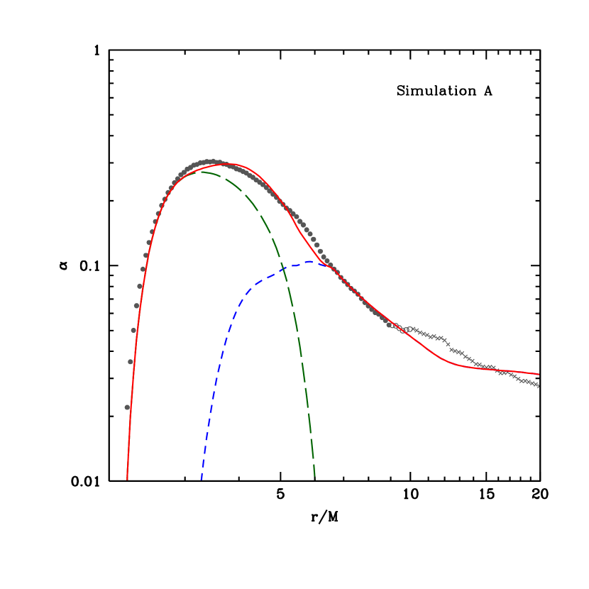
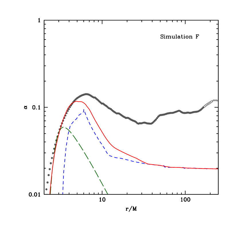
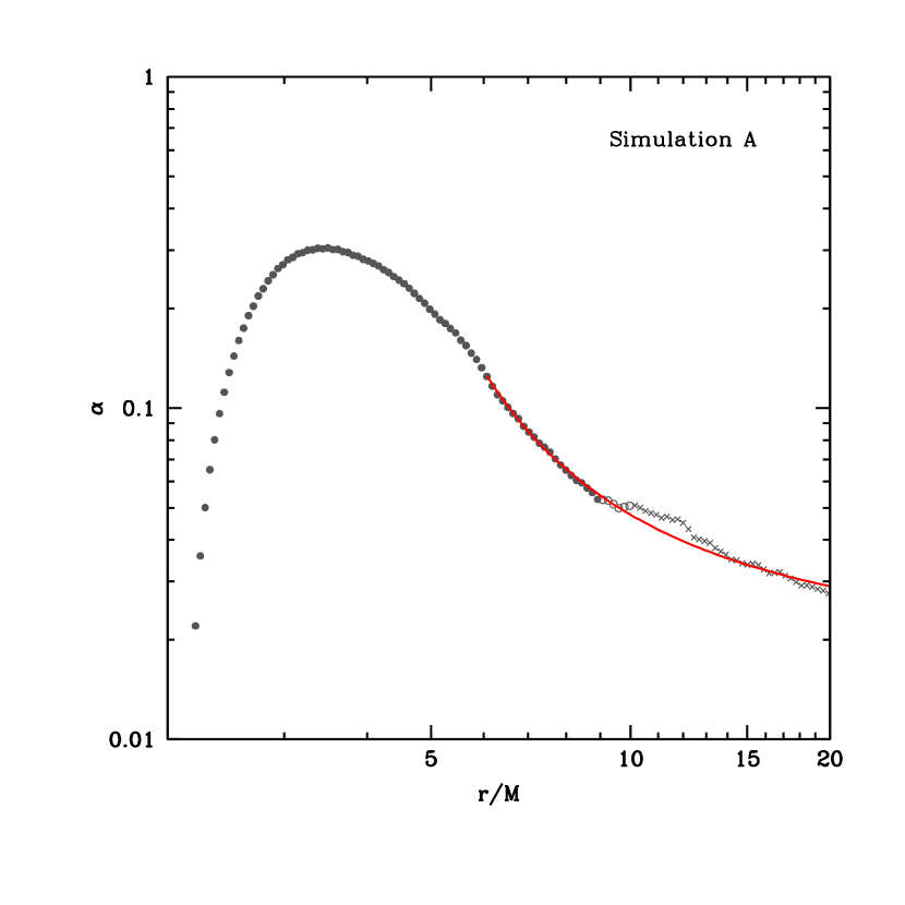
In §§4-6, we estimate values for these four parameters by fitting the $\alpha(r)$ prescription to data from six GRMHD simulations. As an example, Figure 1 shows $\alpha(r)$, as prescribed by equation (30), for the parameters of Model A in Table LABEL:tab:afits (solid red curve). The mean magnetic field contribution to $\alpha(r)$ (long-dashed green curve) dominates inside the ISCO, where the plunging fluid stretches and amplifies the magnetic field. The turbulent contribution to $\alpha(r)$ (dashed blue curve) dominates outside the ISCO, where mean magnetic fields are weak. At large radii, the shear parameter becomes $3/2$ and $\alpha$ becomes constant. Data from a GRMHD simulation (gray points; c.f. §5.5) are in good agreement with the one-dimensional prescription for $\alpha(r)$.

In the next three sections, we detail our GRMHD simulations and their connection to the $\alpha(r)$ prescription.

Figure 1: The $\alpha(r)$ prescription defined by equation (30), for parameters $\alpha_{0}=0.025$, $\alpha_{1}=100$, $n=6$, and $r_{B}=6M$ (solid red curve). This prescription is the sum of two terms, a mean magnetic field component (long-dashed green), which dominates inside the ISCO, and a turbulent component (dashed blue), which dominates outside the ISCO. These two components are based on the one-dimensional models of Gammie (1999) and Sadowski (2011), respectively. At large radii, $\alpha(r)$ converges to $\alpha_{0}=0.025$, a constant. This model is a good description of the data from simulation A (gray points; c.f. §5). Data from inside $r_{\rm strict}$ are marked with filled circles, data from between $r_{\rm strict}$ and $r_{\rm loose}$ are marked with open circles, and data from outside $r_{\rm loose}$ are marked with crosses (c.f. §5.5).

4 Details of the simulations

4.1 Computational Method

The simulations were carried out with the 3D GRMHD code HARM (Gammie et al., 2003; McKinney, 2006; McKinney & Blandford, 2009), which solves the ideal MHD equations for the motion of a magnetized gas in the Kerr metric, the spacetime of a rotating black hole. The equation of motion of the gas is taken to be $u=p/(\Gamma-1)$, where $u$ and $p$ are the internal energy and pressure and $\Gamma$ is the adiabatic index. The code conserves energy to machine precision, so any energy lost at the grid scale by, e.g., turbulent dissipation or numerical reconnection, is returned to the gas, increasing its entropy.

Table LABEL:tab:sims gives a summary of the six simulations, which we have labeled A–F. Simulations A, B, and C are thin, radiatively efficient disks, and simulations D, E, and F are thick, radiatively inefficient disks. The spin parameter is $a/M=0.7$ for simulations B and E, and $a/M=0$ for the others.

Table 1: GRMHD simulation parameters

Simulation	$a/M$	$h/r$	Initial loops	$n_{r}\times n_{\theta}\times n_{\phi}$	$\phi_{\rm max}$	Duration
A	0	0.1	Multiple	$256\times 128\times 64$	$\pi$	$20,000M$
B	0.7	0.05	Multiple	$256\times 64\times 32$	$\pi/2$	$27,000M$
C	0	0.05	Multiple	$256\times 64\times 32$	$\pi/2$	$27,000M$
D	0	0.3	Multiple	$256\times 128\times 64$	$2\pi$	$200,000M$
E	0.7	0.3	Multiple	$256\times 128\times 64$	$2\pi$	$100,000M$
F	0	0.3	Single	$264\times 126\times 60$	$2\pi$	$100,000M$

Most of the simulations have been described in previous papers, so our overview of the simulations in this section can be brief. Simulations B and C are two of the models discussed by Kulkarni et al. (2011). Simulations A, B, and C were analyzed by Zhu et al. (2012) (where they are labeled E, B, and C, respectively). Finally, simulations D and F were studied by Narayan et al. (2012) (where they are called SANE and MAD). The only simulation that has not appeared before is E, but it only differs from D in that it has $a/M=0.7$ and a duration of $100,000M$.

The resolution of simulations B and C in $r\times\theta\times\phi$ is $256\times 64\times 32$, and the resolution of the other simulations is $256\times 128\times 64$. The radial grid is logarithmically spaced to concentrate attention on the inner regions of the flow. The inner boundary of the grid is between the Cauchy horizon and event horizon, and outflow boundary conditions are used there, so the event horizon behaves as a true horizon. The polar grid is squeezed towards the equatorial plane to concentrate resolution on the turbulent, high density regions of the flow, at the expense of the laminar, coronal regions. Simulations D, E, and F use a version of the grid developed by Tchekhovskoy et al. (2011), in which the $\theta$ resolution near the pole increases with increasing radius so as to follow the formation of jets, which collimate at large distances. The azimuthal grid is uniform and extends from 0 to $\phi_{\rm max}$, where $\phi_{\rm max}$ is either $\pi/2$ (simulations A, B, and C) or $2\pi$ (simulations D, E, and F).

The properties of the six simulations are summarized in Table LABEL:tab:sims.

4.2 Initial Conditions

Initially, the gas orbits the black hole in a torus in hydrostatic equilibrium (De Villiers et al., 2003; Penna et al., 2010, 2012a). The thickness of the torus can be adjusted to give either thin or thick accretion disks. A weak poloidal magnetic field threads the torus. All of the simulations start with a sequence of poloidal loops, except F, which starts from a single magnetic loop. When there are multiple loops, the black hole accretes flux of alternating polarity over time and little net flux builds up on the hole. In simulation F, the center of the loop at $r=300M$ does not reach the black hole over the duration of the simulation, so the black hole acquires a large net flux. In all of the simulations, the magnetic field is normalized so that the initial gas-to-magnetic pressure ratio has minimum $\beta=100$.

4.3 Quasi-Steady State

The initial condition is unstable to the MRI. Differential rotation of the torus triggers the MRI and the gas becomes turbulent after $\sim 10$ orbits. Turbulence transports angular momentum and energy outwards and the gas accretes inwards. At late times in the simulation, gas in the disk near the midplane is turbulent. Magnetic buoyancy lifts fields above and below the disk, forming a highly magnetized corona. The corona is mostly laminar because the MRI requires $\beta>1$.

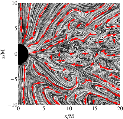
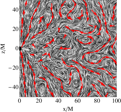
Figure 2 shows the fluid frame magnetic field at the end of simulations A and D. The field has been azimuthally averaged but not time averaged. The coordinates are $x/M=r\sin(\theta)$ and $z/M=r\cos(\theta)$. The turbulent region of simulation A is thinner than the turbulent region of simulation D. The turbulent region of simulation D extends nearly to the polar axes.

Figure 2: Left panel: Black, white, and red streamlines show the poloidal, fluid frame magnetic field $(b^{\hat{r}},b^{\hat{\theta}})$ for simulation A. The field has been azimuthally averaged to make the streamlines appear continuous in this two-dimensional projection (this makes the flow appear slightly less turbulent). Turbulent twisting of the magnetic field can be seen on different scales. When the field is twisted on the smallest scale, the grid scale, there is reconnection and dissipation. The density scale height of the disk is $h/r\sim 0.1$ (c.f. §5.1). Fluid in the disk region of the flow is turbulent. Magnetic buoyancy lifts magnetic fields out of the disk where they settle in a highly magnetized coronal region. The coronal region is mostly laminar, because magnetic tension is quenching the MRI. On very large scales, the magnetic field has an approximately dipolar structure. Right panel: Same as left panel, but for simulation D. This accretion flow is much thicker and the flow only becomes laminar near the polar axes.

5 Analysis of Simulations A and D

In this section we discuss our analysis of simulations A and D. These describe a prototypical thin disk and a prototypical thick disk around non-spinning black holes. We discuss the remaining four simulations in §6

Our goal for this section, achieved in §5.6, is to extract $\alpha(r)$ profiles from the simulation data and compare them with the one-dimensional prescription defined by equation (30). As a first step, we discuss the distinction between disk and coronal fluid. We only include disk fluid in our calculations. Then we discuss the radial range of fluid that can be considered to have reached a quasi-steady state. We only include quasi-steady data in our calculations. We examine the shear rate and epicyclic frequency of the simulations, because these play an important role in determining $\alpha$. Finally, we compute $\alpha(r)$ and compare it with our prescription from §3

5.1 The Distinction Between Disk and Corona

We would like to separate the disk component of the flow from the coronal component so that we can focus our analysis on the disk. There are several reasons to do this. For one, the stress has a different character in the corona and disk regions of the flow. In the corona, the stress is mostly generated by mean magnetic fields, while in the disk, the stress is generated largely by turbulence. So including coronal stresses in the model would add new difficulties. For this reason, and also for simplicity, we focus on the disk region of the flow.

There are other reasons to isolate the disk from the corona. At least in thin accretion disks, the emission from the corona and disk are different. The disk has a thermal spectrum and the corona has a power law spectrum. So the distinction is sensible for observations. Accretion disk models which use the $\alpha$-viscosity prescription tend to focus on the disk region of the flow and ignore the corona. Another reason to separate out the disk region is that our numerical grid concentrates $\theta$ resolution at the midplane and leaves the polar regions poorly resolved. So the simulation data are unreliable in the corona.

We therefore only include fluid within one density scale height of the midplane in our analysis. The density scale height is defined as,

$$\frac{h}{r}=\frac{\int_{0}^{2\pi}\int_{0}^{\phi_{\rm max}}\int_{t_{1}}^{t_{2}}\left|\theta-\pi/2\right|\rho u^{t}\sqrt{-g}dtd\theta d\phi}{\int_{0}^{2\pi}\int_{0}^{\phi_{\rm max}}\int_{t_{1}}^{t_{2}}\rho u^{t}\sqrt{-g}dtd\theta d\phi}.$$ (31)

where $\rho$ is rest mass density in the fluid frame, and $\rho u^{t}$ is rest mass density in Boyer-Lindquist coordinates. The time integral is over the steady state period of the flow, as explained below. Another popular definition for the scale height is $\left(h/r\right)_{\rm rms}=\left(\int\left(\theta-\pi/2\right)^{2}\rho\sqrt{-g}dtd\theta d\phi/\int\rho\sqrt{-g}dtd\theta d\phi\right)^{1/2}$. We have no reason to favor one definition over another, though it should be noted that $(h/r)_{\rm rms}$ can be a factor of $\sim 2$ bigger than $h/r$ (Penna et al., 2010).

We also add a density-weighting to vertical averages, to further emphasize midplane fluid. That is, the density weighted vertical average of $\mathcal{O}$ is $\int\mathcal{O}\rho u^{t}\sqrt{g_{\theta\theta}}d\theta/\int\rho u^{t}\sqrt{g_{\theta\theta}}d\theta$.

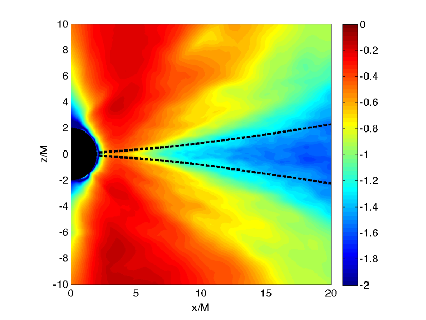
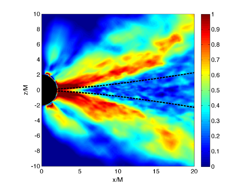
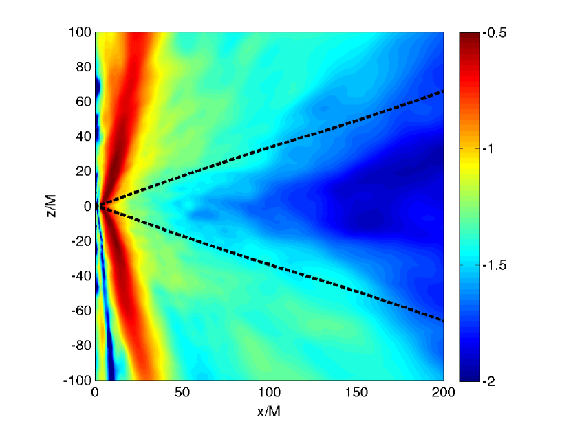
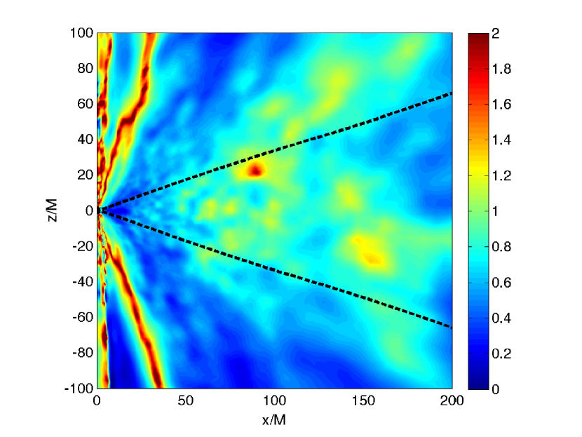
The top panel of Figure 3 shows $\log(\alpha)$ as a function of $x$ and $z$ for simulation A. We explain how $\alpha$ is obtained from the simulation in §5.5, but we show this plot here to illustrate the distinction between the disk and the corona. Black dashed curves mark one scale height above the midplane. Note that $\alpha$ has a very different character above and below the disk region. In the coronal regions $\alpha$ is much larger than in the disk. The bottom panel of Figure 3 shows the ratio of Maxwell stress to Reynolds stress on a logarithmic scale. Maxwell stresses are much more significant in the corona. The different character of the flow in these two regions is one of the reasons we only include disk fluid within one $h/r$ of the midplane in our calculations.

Figure 4 shows the same quantities for simulation D. Again, $\alpha$ and the Maxwell stress are much larger outside the disk. However, the shape of this region does not track $h/r$ as it did in simulation A. In fact, the high $\alpha$, high Maxwell stress region has a parabolic shape, bounded by roughly $z/M=\left(r/6M\right)^{2}$. This looks like a jet. For simplicity and consistency, we will restrict our calculations to the fluid within one $h/r$ of the midplane for all of the simulations. We have checked that our results do not depend on the details of this cutoff, as long as we do not include the “jet” region.

Figure 3: Top panel: $\log(\alpha)$ in the $r-\theta$ plane for simulation A. The data has been time-averaged over $t=7,000M-20,000M$. Dashed black lines indicate one density scale height above and below the midplane (c.f. §5.1). We refer to the low $\alpha$ region within one scale height of the midplane as the disk, and the high $\alpha$ region outside one scale height as the corona. We restrict our calculations to the disk, for the reasons discussed in §5.1. We show this plot here to illustrate the difference between the disk and the corona. We explain how $\alpha$ is obtained from the simulation in §5.5. Bottom panel: Time-averaged ratio of Maxwell stress to Reynolds stress on a log scale, in the $r-\theta$ plane, for simulation A. Coronal fluid is more magnetically dominated than disk fluid. This is expected, as magnetic buoyancy lifts magnetic fields into the corona.

Figure 4: Same as Figure 3, except for simulation D. Unlike simulation A, the highly magnetized region does not have the same shape as the disk scale height. In fact, the former has a paraboloidal, jet-like shape, approximately $z/M=\left(r/6M\right)^{2}$.

5.2 Radial and Azimuthal Velocities

To extract smooth results from turbulent data, it is necessary to average the data over at least a viscous time, which smooths out turbulent fluctuations (Narayan et al., 2012). As a first step, we need the radial velocity of the simulations. To compute the shear rate and epicyclic frequency of the gas (and thus $\alpha$), we need the azimuthal velocity of the gas. We compute these two components of the velocity in this section. We will not need the $\theta$ component of the velocity. It is much smaller than the radial and azimuthal components in the disk region of the flows.

In a thin accretion disk, the gas closely follows circular geodesics as it spirals toward the ISCO. The radial velocity of the gas is significantly smaller than the azimuthal velocity. In a standard thin disk, the radial velocity is suppressed by a factor of $\alpha(h/r)^{2}$. In the ADAF solution, which describes a very thick accretion flow, the radial velocity is suppressed by a factor of $\alpha$ relative to the azimuthal velocity. These relations hold approximately for the GRMHD simulations as well.

The radial velocity most relevant for turbulence is the one measured by the zero angular momentum observer (ZAMO) of Bardeen et al. (1972). This is a local, inertial frame attached to observers with zero angular momentum. As a result of frame dragging, ZAMO observers appear to rotate with respect to observers at infinity. The ZAMO frame is at rest with respect to the local spacetime.

The radial velocity in the ZAMO frame is

$$v_{r}=\frac{\sqrt{A}}{\Delta}\frac{u^{r}}{u^{t}},$$ (32)

where $\Delta$ and $A$ are defined by equations (2) and (4).

The top left panel of Figure 5 shows the radial velocity as a function of radius for simulation A. The data has been averaged over the disk region of the flow, with a density weighting, as discussed in §5.1. It has been time-averaged over the quasi-steady state period of the flow, which we explain below. The ISCO is at $r=6M$. Inside the ISCO, the gas is approximately in free fall and the radial velocity increases rapidly as the gas approaches the black hole. Outside the ISCO, the motion is more nearly circular. In this region, the radial velocity is suppressed relative to the azimuthal velocity as predicted by standard disk theory. Because the radial velocity is small, it takes a long time for the simulation to reach a quasi-steady state. Once steady state is reached, it requires a time average extending over many orbital periods to smooth out turbulent fluctuations and obtain reliable results. We take up these issues in the next section.

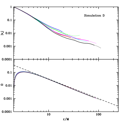
The top right panel of Figure 5 shows the radial velocity as a function of radius for simulation D. The radial velocity is much larger than the radial velocity of A, because this accretion flow is geometrically thick. For this reason, the data from this simulation is in quasi-steady state out to a larger radius. Also, the larger radial velocity smears out the inner edge of the accretion disk. There is no longer a sudden transition between slow and fast radial velocity, at the ISCO or at any other radius.

The bottom left panel of Figure 5 shows the angular velocity

$$\Omega=\frac{d\phi}{dt}=\frac{u^{\phi}}{u^{t}},$$ (33)

of simulation A as a function of radius. Again, we have included only fluid within one scale height of the midplane, taken the density-weighted vertical average, and time averaged over the steady state portion of the flow. The dashed line shows the angular velocity of circular geodesics in the equatorial plane, $\Omega=M^{1/2}/(r^{3/2}+aM^{1/2})$. The flow follows circular geodesics except for $r\lesssim 5M$, where the radial velocity is increasing rapidly. The angular velocity peaks around $3M$. At this radius, the shear parameter $q$ must go to zero, so the turbulent contribution to $\alpha$ becomes negligible.

The bottom right panel of Figure 5 shows the angular velocity of simulation D. It is also nearly Keplerian outside the ISCO. This is perhaps surprising, because the angular velocity of the self-similar ADAF solution is very sub-Keplerian. The initial torus of the GRMHD simulation persists at large radii over the duration of the simulation and continues to feed nearly Keplerian gas into the inner regions of the flow. This acts as a very strong boundary condition, which may limit the solution’s ability to converge to the ADAF solution. The ADAF solution is self-similar and describes an accretion flow with infinite extent but, as we will see, the simulation is only converged out to $r=100M$. A longer duration simulation, which has reached quasi-steady state out to a larger radius, might be expected to have a more ADAF-like angular velocity. Nonetheless, the radial velocity of simulation D does appear to be converging to the ADAF prediction, as shown by Narayan et al. (2012).

Figure 5: Top left: Radial velocity as a function of radius for simulation A. The solid line extends to $r=r_{\rm strict}$ and the dashed line extends to $r=r_{\rm loose}$ (estimated convergence radii of §5.3). The radial velocity increases suddenly around the ISCO at $r=6M$, inside of which there are no stable circular orbits for the gas to follow. Top right: Radial velocity as a function of radius for simulation D. Colors correspond to time chunks 1 (blue), 2 (green), 3 (red), 4 (cyan), 5 (magenta), and 6 (black) (see §5.3). Bottom left: Angular velocity as a function of radius for simulation A. The dashed black curve shows the angular velocity of circular, equatorial geodesics. The simulated flow is nearly geodesic outside the ISCO. The angular velocity has a maximum near the photon orbit at $r=3M$, so the shear parameter (and hence the turbulent contribution to $\alpha$) will be zero here. Bottom right: Angular velocity as a function of radius for simulation D. This flow is slightly sub-Keplerian outside the ISCO.

5.3 Convergence and Steady State

Following Narayan et al. (2012), we divide the data from simulation D into six “time chunks” which are logarithmically spaced in time. Each time chunk is about twice as long as the previous one. They are summarized in Table LABEL:tab:sane. This logarithmic spacing is useful since most of the quantities we are interested in show power-law behavior as a function of both time and radius. Note that there is no overlap between chunks, and hence each chunk provides independent information. Because the duration of simulation A is only $20,000M$, we use a single time chunk, spanning $t=7,000M-20,000M$.

For each time chunk, we compute the time-averaged radial velocity profile $v_{r}(r)$ of the gas within one scale-height of the mid-plane. We estimate the viscous time at radius $r$ by (Novikov & Thorne, 1973; Penna et al., 2010):

$$t_{\rm visc}(r)=\frac{r}{|v_{r}(r)|}.$$ (34)

Following Narayan et al. (2012), we then define two criteria, one “strict” and one “loose,” to estimate the radius range over which the flow has achieved inflow equilibrium:

$$t_{\rm visc}(r_{\rm strict}) =t_{\rm chunk}/2,$$ (35)

$$t_{\rm visc}(r_{\rm loose}) =t_{\rm chunk},$$ (36)

where $t_{\rm chunk}$ is the duration of the chunk. The values of $t_{\rm chunk}$, $r_{\rm strict}$, and $r_{\rm loose}$ for the various time chunks are summarized in Tables LABEL:tab:thin and LABEL:tab:sane. We only trust data from inside $r_{\rm loose}$. Data from inside $r_{\rm strict}$ are considered particularly reliable.

Table 2: Convergence radii for simulations A, B, and C

Simulation	Time Range (M)	$t_{\rm chunk}/M$	$r_{\rm strict}/M$	$r_{\rm loose}/M$
A	7,000-20,000	13,000	9	10
B	20,000-27,000	7,000	6.5	7
C	20,000-27,000	7,000	6.5	7

Table 3: Time chunks for simulation D

Chunk	Time Range (M)	$t_{\rm chunk}/M$	$r_{\rm strict}/M$	$r_{\rm loose}/M$
I	3,000-6,000	3,000	19	23
II	6,000-12,000	6,000	25	43
III	12,000-25,000	13,000	29	45
IV	25,000-50,000	25,000	43	62
V	50,000-100,000	50,000	66	92
VI	100,000-200,000	100,000	86	113

5.4 Shear and Epicyclic Frequencies

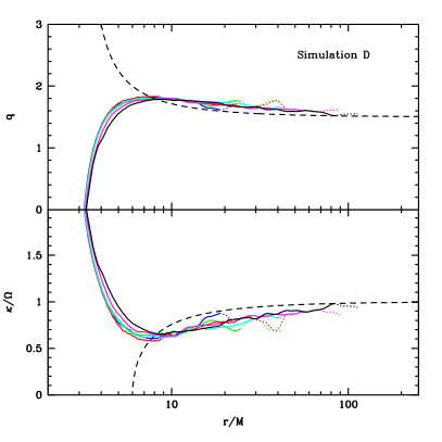
Now we compute the dimensionless shear parameter, $q$, and the epicyclic frequency, $\kappa$, as a function of radius. The shear parameter is computed from $q=-2\sigma_{\hat{r}\hat{\phi}}/\Omega$. The epicyclic frequency is computed from the shear parameter using equation (25). The data are vertically averaged over the gas within one scale height of the midplane using the density weighting. The data are time averaged over the time chunks listed in Tables LABEL:tab:thin and LABEL:tab:sane.

The top left panel of Figure 6 shows the shear parameter as a function of radius for simulation A out to $r_{\rm strict}$ (solid curve) and $r_{\rm loose}$ (dotted curve). The analytical shear parameter for circular, equatorial Kerr geodesics is shown for comparison (dashed curve). At large radii, the analytical $q$ converges to the shear parameter of non-relativistic Keplerian flow, $q=3/2$. At the ISCO, general relativistic corrections increase the shear parameter to $q=2$. The GRMHD shear parameter is about $10\%$ larger than the analytical shear parameter outside the ISCO. Inside the ISCO, the analytical $q$ blows up as it approaches the photon orbit. The GRMHD shear parameter goes to zero near the photon orbit and is negative very close to the black hole.

The top right panel of Figure 6 shows the shear parameter as a function of radius for simulation D. Results are shown for each of the time chunks. All of the time chunks are consistent out to $r_{\rm loose}$ to within several percent. This gives us confidence that the simulation has converged to a quasi-steady solution. The GRMHD shear parameter is similar to the shear parameter of simulation A. It is about $10\%$ larger than the analytical $q$ outside the ISCO, turns over inside the ISCO, and drops to zero near the photon orbit. There is good agreement between the GRMHD and analytical shear parameters out to $r_{\rm loose}\sim 100M$.

The bottom left panel of Figure 6 shows the epicyclic frequency as a function of radius for simulation A. The bottom right panel shows the same quantity for simulation D. In both cases, outside the ISCO, the epicyclic frequency of the simulation is about $10\%$ lower than the epicyclic frequency of Keplerian flow. In both cases the epicyclic frequency has a minimum near the ISCO. The minimum of the epicyclic frequency roughly marks the most unstable radius in the flow, because $\kappa=0$ corresponds to marginal stability. So it is consistent with standard disk theory that the minimum of $\kappa$ is near the ISCO. Simulation D has a broader and shallower minimum, indicating the inner edge of this disk has been “smeared out” by the larger radial velocity of the flow.

Figure 6: Top left: Dimensionless shear parameter, $q$, as a function of radius for simulation A (solid and dotted curves) and for Keplerian flow (dashed). The simulation data are plotted out to $r_{\rm loose}$ (dotted curves) and out to $r_{\rm strict}$ (solid curves). The simulated shear parameter turns over near the ISCO. Top right: Dimensionless shear parameter as a function of radius for simulation D. Colors are as in Figure 5. Bottom left: Epicyclic frequency as a function of radius for simulation A. The epicyclic frequency has its minimum near the ISCO, as expected. Bottom right: Epicyclic frequency as a function of radius for simulation D. The minimum is still near the ISCO, but it is broader and shallower than the minimum in the epicyclic frequency of simulation A. The larger radial velocity of simulation D has “smeared out” the inner edge of the disk.

5.5 Shakura-Sunyaev Viscosity Parameter, $\alpha$

Finally, we compute the dimensionless viscosity parameter, $\alpha$. The GRMHD stress-energy tensor is a combination of Reynolds and Maxwell terms:

$$T_{\mu\nu}=T^{\rm(rey)}_{\mu\nu}+T^{\rm(mag)}_{\mu\nu},$$ (37)

where,

$$T^{\rm(rey)}_{\mu\nu} =(\rho+u)u_{\mu}u_{\nu}+ph_{\mu\nu},$$ (38)

$$T^{\rm(mag)}_{\mu\nu} =\frac{1}{2}\left(b^{2}u_{\mu}u_{\nu}+b^{2}h_{\mu\nu}-2b_{\mu}b_{\nu}\right),$$ (39)

and $h_{\mu\nu}=g_{\mu\nu}+u_{\mu}u_{\nu}$ is the projection tensor. To each term there is an associated stress, which is the $r\phi$ component of the tensor measured in the fluid frame. So the Reynolds stress is $T^{\rm(rey)}_{{\hat{r}}{\hat{\phi}}}$ and the Maxwell stress is $T^{\rm(mag)}_{{\hat{r}}{\hat{\phi}}}$. An important difference between the two is that the Reynolds stress requires turbulence whereas the Maxwell stress can be generated by turbulence or large scale magnetic fields and thus can be nonzero even in laminar flow.

We define $\alpha$ as the ratio of total stress to total pressure:

$$\alpha=\frac{T^{\rm(rey)}_{{\hat{r}}{\hat{\phi}}}+T^{\rm(mag)}_{{\hat{r}}{\hat{\phi}}}}{p+b^{2}/2}.$$ (40)

We have chosen to include $b^{2}/2$ in the denominator because it keeps $\alpha<1$. As a result of this choice, part of the observed dependence of $\alpha$ on $q$ is inherited via the magnetic pressure because the magnetic pressure is amplified by shear. This is significant inside the ISCO where the magnetic pressure is comparable to or exceeds the gas pressure.

We compute the Maxwell and Reynolds stresses in the rest frame of the mean flow,

$$\bar{u}^{\mu}=\frac{1}{\phi_{\rm max}}\int_{0}^{\phi_{\rm max}}u^{\mu}d\phi,$$ (41)

rather than in the rest frame of the instantaneous flow, $u^{\mu}$. The mean flow is the $\phi$-averaged instantaneous flow. There are some subtleties in the distinction between these two frames. The Reynolds stress vanishes in the rest frame of the instantaneous flow, $u^{\mu}$, by definition of the fluid frame, but not in the rest frame of the mean flow, $\bar{u}^{\mu}$. This is our primary reason for choosing $\bar{u}^{\mu}$ to define the inertial fluid frame when computing $\alpha$ . The electric field vanishes in the rest frame of the instantaneous flow, by the assumption of ideal MHD, and not in the rest frame of the mean flow, but for simplicity we assume the electric field can be neglected in both frames.

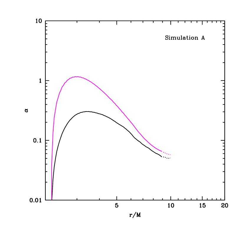
One could include a time average in the definition of the mean flow, equation (41). Penna et al. (2010) included a $100M$ time average. That is, they averaged the instantaneous flow over all of $\phi$ and over $100M$ in time to obtain the mean flow. At large radii, $100M$ is much smaller than the orbital timescale, so this extra averaging has little effect. However, inside the ISCO, $100M$ is larger than the orbital timescale. In this case, the time-averaged mean flow tends to give larger $\alpha$. The reason is that time-averaging increases the discrepancy between the mean and instantaneous flows by adding contributions to the mean flow from earlier and later times. This discrepancy propagates into $\alpha$ when the stress tensor is boosted to the rest frame of the mean flow.

Figure 7 shows $\alpha(r)$ for simulation A with and without a $100M$ time averaging in the definition of $\bar{u}^{\mu}$. Including the time averaging increases $\alpha$ and the effect is greatest inside the ISCO. In fact, the peak $\alpha$ exceeds unity when the mean flow is defined with a time average. This would imply the stresses carry more energy than the total energy of the gas and magnetic fields, which is unphysical. To avoid these sorts of contradictions, we do not include any time averaging in equation (41).

Figure 7: Dimensionless viscosity parameter, $\alpha$, as a function of radius for simulation A, with (magenta) and without (black) a $100M$ time-average in the definition of the mean fluid frame, $\bar{u}^{\mu}$. Outside the ISCO, $100M$ is longer than an orbital period, so the effect is small. Inside the ISCO, $100M$ is several orbital periods, so the effect is large.

The middle panel of Figure 8 shows the ratio of Maxwell stress to Reynolds stress in simulation A. Outside the ISCO, the ratio tracks the prediction of the linearized MRI, $(4-q)/q$ (Pessah et al., 2006b). In fact, it is slightly larger, as is consistent with shearing box simulations of MRI turbulence (Pessah et al., 2006b). Inside the ISCO, the Maxwell stress is an order of magnitude larger than the Reynolds stress. The flow is mostly laminar inside the ISCO, so Reynolds stress is weak, and the plunging fluid stretches the magnetic field, so the Maxwell stress is strong. The bottom panel of Figure 8 shows the product $\alpha\beta$. It approaches the expected value of $\approx 0.5$ in the disk (Blackman et al., 2008; Guan et al., 2009; Sorathia et al., 2012).

Figure 8: Top panel: Dimensionless viscosity parameter, $\alpha$, as a function of radius for simulation A. The data has been time averaged from $t=7,000M$ to $20,000M$. Solid and dotted curves correspond to $r\leq r_{\rm strict}$ and $r\leq r_{\rm loose}$, Middle panel: Time-averaged ratio of Maxwell to Reynolds stress for simulation A (solid and dotted curves). The dashed curve is the the prediction from a linearized MRI analysis, $4/q(r)-1$ (Pessah et al., 2006b), for Keplerian $q(r)$, equation (24). Bottom panel: Product $\alpha\beta$ for simulation A (solid and dotted curves). The dashed line at $\alpha\beta=0.5$ is the expected value for saturated MRI turbulence (Blackman et al., 2008; Guan et al., 2009; Sorathia et al., 2012). The simulated product falls below this value inside the ISCO where the flow is mostly laminar.

The top panel of Figure 9 shows $\alpha(r)$ for the six time chunks of simulation D. Outside the ISCO, the various time chunks agree to within $30\%$, which provides an estimate for the contribution of turbulent noise to the error in our $\alpha$ measurements. Inside the ISCO, where the flow is more nearly laminar, the agreement between the time chunks is better.

The bottom panel of Figure 9 shows the ratio of Maxwell to Reynolds stress as a function of radius for simulation D. Inside about $r=22M$, the ratio is consistent with the ratio of simulation A. Outside $r=22M$, the ratio begins to grow with radius. It is not clear what causes this. It may indicate that simulation D has not reached quasi-steady state at these radii yet. Figure 4 shows highly magnetized, irregular clumps of fluid in the disk region, even after time-averaging the data over the last time chunk. In a true quasi-steady state, one would expect time averaging to eliminate these clumps.

Figure 9: Same as Figure 8 but for simulation D. Colors and line types are as in Figure 5.

5.6 Comparison With the One-Dimensional $\alpha(r)$ Prescription

Finally, we compare $\alpha(r)$ of the simulations with the one-dimensional prescription for $\alpha(r)$ of §3, as defined by equation (30) and the parameters listed in Table LABEL:tab:afits.

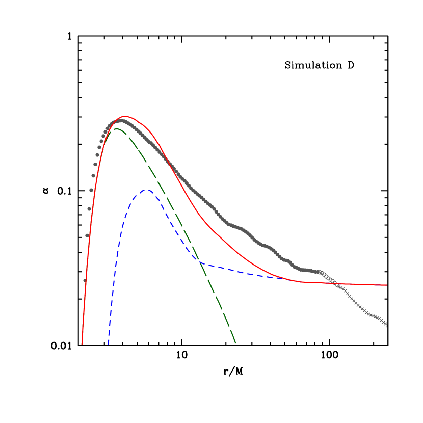
Figure 1 shows the agreement between the GRMHD $\alpha(r)$ from simulation A and the $\alpha(r)$ prescription. Figure 10 shows the agreement between simulation D and the $\alpha(r)$ prescription. The interpretation of the GRMHD $\alpha(r)$ in terms of a mean magnetic field component in the inner regions, and a turbulent component in the outer regions, appears to match the data. It is more difficult to fit simulation D because the $\alpha(r)$ prescription relies on a sharp distinction between the laminar, magnetically dominated inner regions of the flow, and the turbulent, weakly magnetized outer regions. This distinction is cleanest in thin disks, like simulation A, which have a clear inner edge at the ISCO. In thick disks, like simulation D, the inner edge of the disk is smeared out by the radial velocity of the flow, so the separation of $\alpha$ into two independent components is less sound.

The shape of $\alpha(r)$ does not depend strongly on all of the parameters in Table LABEL:tab:afits. The mass of the black hole in the GRMHD simulations is dimensionless. It is listed in Table LABEL:tab:afits because it goes into the slim disk solutions that underlie the one-dimensional $\alpha(r)$ prescription. We set $M/M_{\odot}=10$ arbitrarily and this choice has a negligible effect on $\alpha(r)$.

The accretion rate also enters through the slim disk part of $\alpha(r)$. Our estimates of $\dot{M}/\dot{M}_{\rm edd}$ for the GRMHD simulations are based on the analysis of Zhu et al. (2012), who used $h/r$ as a proxy for the accretion rate. This gives rough estimates, which is all we need because the dependence of $\alpha(r)$ on the accretion rate is also very weak.

The magnetic flux threading the horizon, $\Upsilon$, is measured directly from the GRMHD simulations. It slightly affects the shape of $\alpha(r)$ inside the ISCO.

The four parameters that strongly control the shape of $\alpha(r)$ are $\alpha_{0}$, $\alpha_{1}$, $n$ and $r_{B}$. It is encouraging that $\alpha_{0}=0.025$, and $n=6$ give good fits to both simulations. In other words, both simulations have $\alpha(r)\sim 0.025$ at large radii, and $\alpha\propto q^{6}$ (and $q>0$) in the turbulent disk.

Mean magnetic fields are only important inside the ISCO of simulation A, so we set $r_{B}=6M$ in this case. The region where mean magnetic fields are important in simulation D is broader, so we set $r_{B}=30M$ in this case.

Table 4: Parameters for $\alpha(r)$ fits to the GRMHD simulations

Simulation	$M/M_{\rm\odot}$	$a/M$	$\dot{M}/\dot{M}_{\rm edd}$	$\Upsilon$	$\alpha_{0}$	$\alpha_{1}$	$n$	$r_{B}$
A	10	0	0.5	0.6	0.025	100	6	$r_{\rm ISCO}$
B	10	0.7	0.2	3	0.025	10	6	$r_{\rm ISCO}$
C	10	0	0.2	6	0.025	1	6	$r_{\rm ISCO}$
D	10	0	1	5	0.025	0.5	6	30M
E	10	0.7	1	10	0.025	0.5	6	30M
F	10	0	1	30	0.025	0.1	6	30M

Figure 10: Same as Figure 1 but for simulation D.

6 Analysis of Simulations B, C, E, and F

In this section we present data from four more GRMHD simulations. This gives information about the dependence of the viscosity parameters $\alpha_{0}$, $\alpha_{1}$, $n$, and $r_{B}$, on black hole spin, resolution, and the amount of magnetic flux threading the black hole. Of these effects, the dependence on flux threading the black hole is the most dramatic.

6.1 Simulation E

Simulation E is identical to simulation D except the black hole has spin parameter $a/M=0.7$ and the duration is $100,000M$. We have divided the simulation data into time chunks as we did for simulation D, but there is one less time chunk because the duration is half as long. The time chunks and radii of convergence estimates are listed in Table LABEL:tab:sane7.

Table 5: Time chunks for simulation E

Chunk	Time Range (M)	$t_{\rm chunk}/M$	$r_{\rm strict}/M$	$r_{\rm loose}/M$
I	3,000-6,000	3,000	9.5	15
II	6,000-12,000	6,000	15	20
III	12,000-25,000	13,000	22	31
IV	25,000-50,000	25,000	31	44
V	50,000-100,000	50,000	44	60

Figure 11 shows the radial and angular velocities as a function of radius for the five time chunks. After the first three time chunks, around $t=25,000$, the radial velocity drops by about a factor of 2. Then it holds steady (to within a few percent) for the final two time chunks. So even at $t=25,000M$, the simulation is still settling down. The radial velocity at the end of simulation E is about $30\%$ lower than the radial velocity at the end of simulation D. As a result, simulation E has converged over a smaller range of radii; we find $r_{\rm loose}=60M$ for the last time chunk (simulation D had $r_{\rm loose}=90M$ over the same time interval.)

Figure 11: Same as Figure 5 but for simulation E.

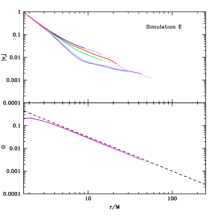
Figure 12 shows the dimensionless shear parameter and epicyclic frequency as a function of radius. Outside the ISCO, the shear parameter is about $20\%$ larger than the shear parameter of circular geodesics and the epicyclic frequency is about $20\%$ smaller, similar to the results from simulation D. The minimum epicyclic frequencies of the two simulations are also comparable. Simulation D had $\kappa/\Omega\sim 0.6$ and simulation E has $\kappa/\Omega\sim 0.5$.

Figure 12: Same as Figure 6 but for simulation E.

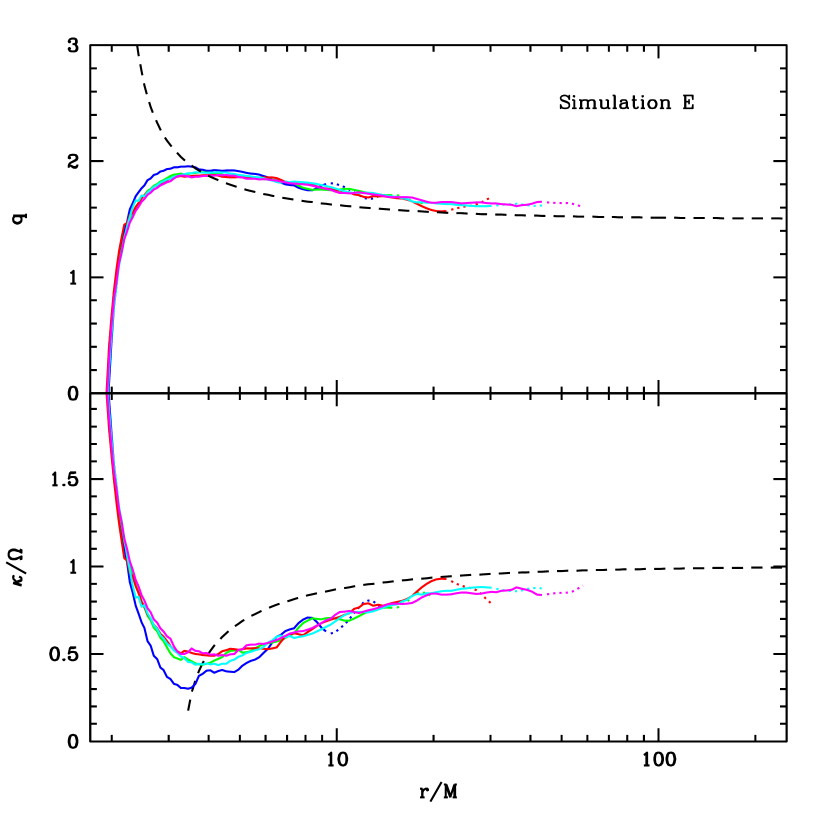
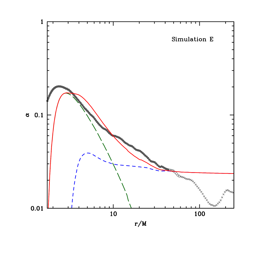
Figure 13 compares $\alpha(r)$ as computed from the last time chunk of the simulation against $\alpha(r)$ computed from the one-dimensional viscosity prescription with $\alpha_{0}=0.025$, $\alpha_{1}=0.5$, $n=6$, and $r_{B}=30M$. This is the same choice of parameters that gave a good fit to simulation D. It is interesting that they fit simulation E as well. This suggests the parameters of the modified viscosity prescription do not depend strongly on black hole spin.

Figure 13: Same as Figure 1 but for simulation E.

6.2 Simulation B

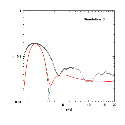
This simulation is identical to simulation A, except the black hole is spinning with spin parameter $a/M=0.7$ and the resolution is $256\times 64\times 32$ rather than $256\times 128\times 64$.

The left panel of Figure 14 shows the GRMHD $\alpha(r)$. The $\alpha(r)$ prescription is shown for the same parameters that gave a good fit to simulation A: $\alpha_{0}=0.025$, $\alpha_{1}=1$, $n=6$, and $r_{B}=r_{\rm ISCO}$. The parameters $\alpha_{0}=0.025$ and $n=6$ governing the turbulent part of $\alpha(r)$ are the same across all four simulations we have considered so far, suggesting these parameters do not depend strongly on disk thickness.

Figure 14: Same as Figure 1 except for simulations B (left panel) and C (right panel).

6.3 Simulation C

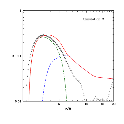
Simulation C is the same as simulation A except the resolution is lower: $256\times 64\times 32$ versus $256\times 128\times 64$ and the disk is thinner ($h/r\sim 0.05$ instead of $h/r\sim 0.1$). The data from this simulation has a lower $\alpha$ than the $\alpha(r)$ prescription with our fiducial choice of parameters $\alpha_{0}=0.025$ and $n=6$. This suggests we are under-resolving the MRI at this resolution. To infer whether the values $\alpha_{0}=0.025$ and $n=6$ are robust, higher resolution simulations would be useful.

The results are shown in the right panel of Figure 14.

6.4 Simulation F

Simulation F differs from simulation D in one crucial respect. The initial torus of gas is threaded with a single poloidal magnetic field loop rather than multiple loops. The center of the initial loop is centered at $r=300M$ and gas from this radius does not reach the black hole over the duration of the simulation. So the polarity of the flux that reaches the black hole is approximately constant and a large net flux builds up on the hole. Narayan et al. (2012) give a detailed account of the convergence in time and radius, and the role of outflows, in simulations D and F.

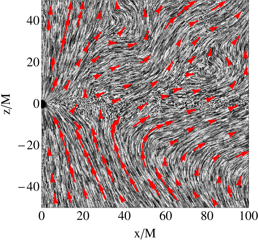
The large net flux carried by the gas in simulation D has a dramatic effect: the flow remains mostly laminar at all radii. Figure 15 shows the fluid frame magnetic field in the $r-\theta$ plane at $t=100,000M$, the final snapshot of the simulation. The eddies and turbulent twisting of the field are all but gone on every scale, in marked contrast to the other five simulations we considered (see, e.g., Figure 2).

Figure 15: Same as Figure 2 but for Simulation F. The magnetic field structure does not show turbulent twisting on any scale; the flow is mostly laminar.

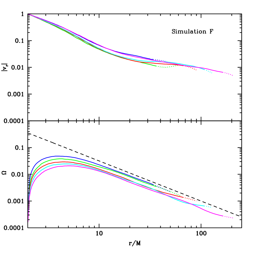
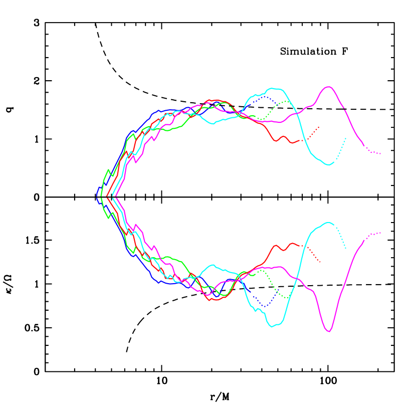
Following Narayan et al. (2012), we divide the simulation data into five time chunks. The time periods and estimated convergence radii for each time chunk are summarized in Table LABEL:tab:mad. This simulation has the largest radial velocity of any of the simulations (see Figure 16), so the estimated convergence radii are the largest. The final time chunk has $r_{\rm strict}=170M$ and $r_{\rm loose}=207M$.

Simulation F also has the most sub-Keplerian angular velocity of the six simulations (Figure 16). The angular velocity drops by a factor of a few between time chunks I and III, but it is consistent across the final three time chunks to within a few percent.

Table 6: Time chunks for simulation F

Chunk	Time Range (M)	$t_{\rm chunk}/M$	$r_{\rm strict}/M$	$r_{\rm loose}/M$
I	3,000-6,000	3,000	35	52
II	6,000-12,000	6,000	37	65
III	12,000-25,000	13,000	69	90
IV	25,000-50,000	25,000	109	128
V	50,000-100,000	50,000	170	207

Figure 16: Same as Figure 5 but for simulation F. Of the six simulations we consider, this simulation has the largest radial velocity and is the most sub-Keplerian.

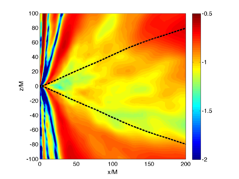
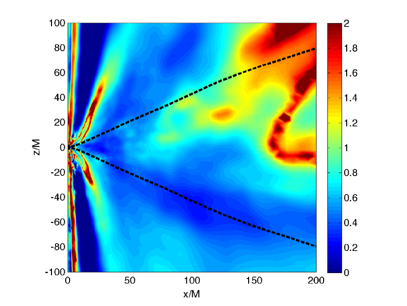
The ratio of Maxwell stress to Reynolds stress has a much clumpier distribution in the $r-\theta$ plane than any of the other simulations. A large, magnetized, z-shaped clump, where the Maxwell stress is enhanced, extends throughout the flow (bottom panel of Figure 17). The irregular shape of the clump suggests it is a non-equilibrium structure. Perhaps if the duration of the simulation was longer it would be smoothed out. The appearance of the magnetized clump suggests $r_{\rm strict}=170M$ is a better estimate for the radii of convergence for this simulation than $r_{\rm loose}=207$.

Figure 17: Same as Figure 3 but for simulation F. A large, highly-magnetized, z-shaped clump persists over most of the flow inside $r_{\rm loose}$. The magnetized clump increases $\alpha$ and the ratio of Maxwell to Reynolds stress.

The shear parameter of the flow (top panel of Figure 18) varies by about $50\%$ between time chunks. Outside the ISCO, the shear parameter is roughly constant with radius. The epicyclic frequency (bottom panel of Figure 18) has its minimum near $r=20M$, rather than at the ISCO. The minimum itself is very broad and shallow, not extending much below $\kappa/\Omega=1$. In other words, the inner edge of the disk has moved well outside the ISCO and is highly smeared out.

Figure 18: Same as Figure 6 but for simulation F.

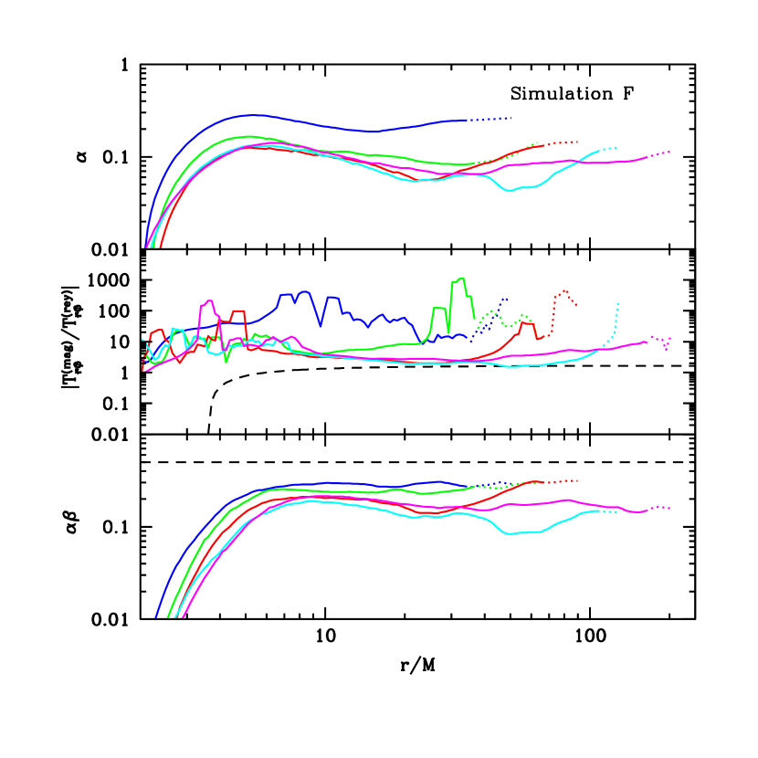
The profiles of $\alpha$ as a function of radius for the five time chunks are shown in the top panel of Figure 19. Outside $r\approx 20M$, the profiles of $\alpha$ are constant with radius, even increasing slightly. The other simulations have $\alpha$ decreasing with radius. This suggests the turbulent contribution to $\alpha$ is not dominating even at the largest converged radii, which is consistent with the laminar structure of the magnetic field lines.

The bottom panel of Figure 19 shows the ratio of Maxwell to Reynolds stress as a function of radius for the five time chunks. For the first two time chunks, the Maxwell stress is an order of magnitude larger than the Reynolds stress at all radii. During the final three time chunks, the ratio appears to have stabilized out to $r=40M$. At larger radii, the Maxwell stress is enhanced by the non-equilibrium, magnetized, z-shaped clump noted earlier.

Figure 19: Same as Figure 8 but for simulation F.

Our $\alpha(r)$ prescription does not appear to give a good fit to the simulation F results (Figure 20). This is probably because the simulation is mostly laminar at all radii (as shown by Figure 15), whereas our $\alpha(r)$ prescription assumes turbulence dominates the stress beyond the innermost radii. For simulations A–E, this is a good assumption provided the disk region of the flow is distinguished from the coronal regions. However, the entire domain of simulation F is mostly laminar and highly magnetized, and so it should perhaps be considered entirely coronal gas. It appears a different $\alpha(r)$ prescription is needed to describe such highly magnetized flows.

Figure 20: The dimensionless viscosity parameter, $\alpha$, of simulation F as a function of radius. We have been unable to find a good fit to the simulation data using our $\alpha(r)$ prescription.

7 $\alpha$-Disk Solutions with Variable $\alpha(r)$

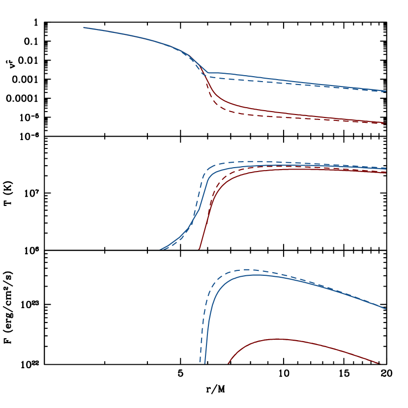
In this section, we evaluate the dependence of $\alpha$-disk solutions on the $\alpha(r)$ prescription. The particular $\alpha$-disks we consider are “slim disks” (Abramowicz et al., 1988; Sadowski, 2011). We compare slim disk solutions with constant $\alpha=\alpha_{0}$ to solutions with varying $\alpha(r)$, where $\alpha(r)$ is defined by equation (30) and the parameters inferred from simulation A (c.f. Table LABEL:tab:afits). That is, we consider a non-spinning, 10 solar mass black hole, threaded with a magnetic flux $\Upsilon=0.6$. The viscosity parameters are $\alpha_{0}=0.025$, $n=6$, $\alpha_{1}=100$, and $r_{B}=6M$. We consider two different accretion rates: $30\%$ Eddington and Eddington.

Figure 21 shows our results. At large radii, $\alpha(r)$ converges to $\alpha_{0}$, so the solutions with constant and varying $\alpha(r)$ are the same to within a percent. Inside the ISCO, the fluid plunges toward the black hole with little dissipation, so in the innermost regions the solutions are again insensitive to the $\alpha$ prescription. Only in an intermediate zone, between the ISCO and $r\approx 20M$, does the shape of $\alpha(r)$ have a significant effect. For solar mass black holes, this region emits predominately in X-rays and is relevant for black hole spin measurements (Gou et al., 2011).

In this zone, the $\alpha(r)$ prescription has a larger $\alpha$ than the constant $\alpha=\alpha_{0}$ prescription. So the $\alpha(r)$ prescription increases the disk’s radial velocity by a factor of $2-3$ and lowers its central (mid-plane) temperature by about $50\%$. In fact, a solution accreting at the Eddington limit with varying $\alpha(r)$ has the same central temperature as a solution accreting at $30\%$ Eddington with constant $\alpha$ (c.f. Figure 21). So the $\alpha(r)$ prescription has a significant effect on central temperature. Central temperature depends on both effective temperature and optical depth, so the effect is really due to changes in surface density.

At low accretion rates, the disk is radiatively efficient and the effect of $\alpha(r)$ on the radiated fluxed is negligible. At high accretion rates, advection becomes important and the radiated flux shows its dependence on $\alpha(r)$. At the Eddington limit, the flux from the solution with varying $\alpha(r)$ is about $50\%$ lower than the flux from the solution with constant $\alpha$. So flux is only affected by the $\alpha(r)$ prescription at high accretion rates.

Figure 21: Slim disk solutions with varying $\alpha(r)$ (solid curves) and with constant $\alpha=0.025$ (dashed curves), for the parameters inferred from simulation A (c.f. LABEL:tab:afits). Solutions are shown at the Eddington accretion rate (blue curves) and at $30\%$ Eddington (red curves). Top panel: Radial velocity as a function of radius. Solutions with varying $\alpha(r)$ have larger radial velocities. Middle panel: Midplane temperature (not effective temperature) as a function radius. Solutions with varying $\alpha(r)$ are colder in the X-ray emitting portions of the flow. Bottom panel: Radiant flux as a function of radius. Radiant flux is affected by $\alpha(r)$ only at high accretion rates.

8 Discussion and summary

The $\alpha(r)$ prescription of §3 must be computed numerically. However, for all practical purposes, the function $\alpha(r)$ for thin disks can be reduced to a simple analytical formula. Our simulations suggest

$$\alpha(r)=0.025\left[\frac{q(r)}{3/2}\right]^{6},\quad(q>0),$$ (42)

where $q(r)$ is given analytically by equation (24). The constant coefficient and exponent in equation (42) are the values favored by our GRMHD simulations (c.f. Table LABEL:tab:afits). They will change as better simulation data becomes available. The free parameters are the mass and spin of the black hole, which enter through equation (24) for $q(r)$. The contribution from mean magnetic fields can be ignored in this approximation because mean field stresses are only significant inside the ISCO, and thin disks are not sensitive to $\alpha(r)$ in this region. Equations (24) and (42) thus give an analytical $\alpha(r)$ prescription that can be used for thin disk models (see Figure 22). The more general $\alpha(r)$ prescription of §3 is needed for thick disks.

Figure 22: Analytical $\alpha(r)$ prescription defined by equation (42) for $a/M=0$ (solid red curve). This model gives a good fit to data from Simulation A. Data from inside $r_{\rm strict}$ are marked with filled circles, data from between $r_{\rm strict}$ and $r_{\rm loose}$ are marked with open circles, and data from outside $r_{\rm loose}$ are marked with crosses (c.f. §5.5).

To summarize our main results, we have constructed a one-dimensional prescription for $\alpha(r)$ and estimated parameters for this prescription based on data from GRMHD simulations. The fact that $\alpha$ varies with radius had been anticipated long ago (Pringle & Rees, 1972; Shakura & Sunyaev, 1973) but global MHD simulations provide the first quantitative information about the shape of $\alpha(r)$ (Papaloizou & Nelson, 2003; Penna et al., 2010, 2012b; Fromang et al., 2011).

Our modified $\alpha(r)$ prescription, equation (30), is the sum of two components. The first component describes mean field stresses. It is important in the laminar, inner regions of accretion disks, where the plunging fluid stretches the frozen-in field. Our description of this component is based on the model of Gammie (1999), which supplies the magnetic stress as a function of radius and two free parameters: black hole spin and the amount of magnetic flux threading the horizon.

The second component of the $\alpha(r)$ prescription describes turbulent stresses. As emphasized by Pessah et al. (2006b), $\alpha$ depends on the shear parameter, $q$. In Newtonian gravity, Keplerian flow has a constant shear parameter, $q=3/2$, but general relativistic corrections give even Keplerian disks around black holes a varying $q(r)$, as discussed in §2. The shear parameter increases from $q=3/2$ at the outer edge of the disk to $q=2$ at the inner edge of the disk. This is a $50\%$ change in $q$ but it creates a larger variation in $\alpha$, because $\alpha$ goes as $q^{n}$ (for $q>0$). Our GRMHD simulations are too noisy to infer $n$ precisely, but the data seem to prefer $n\approx 6$. This is consistent with the simulations of Pessah et al. (2006b), which resulted in $n$ between 2 and 8. Analytical MHD closure models for the MRI also allow $n$ between 2 and 8 (Kato & Yoshizawa, 1993, 1995; Ogilvie, 2003; Pessah et al., 2006a, b, 2008).

Simple extensions of the standard $\alpha$ prescription and some closure models predict negative $\alpha$ for $q<0$ (Kato & Yoshizawa, 1993, 1995; Ogilvie, 2003). An exception is the closure model of Pessah et al. (2006a, b). Data from shearing box simulations show zero turbulent stress for $q<0$ (Pessah et al., 2008). Our simulations are consistent with this data, although they are not as decisive on this point because negative shear parameters are only found inside roughly the photon orbit, where mean field stresses are large. Our prescription for $\alpha(r)$ is always positive and the turbulent contribution vanishes for $q<0$. The mean field term in our $\alpha(r)$ prescription gives a good description of our simulation data in regions near the black hole where $q<0$.

We have discussed accretion onto black holes. When a disk accretes onto a star, a boundary layer forms between the star and disk. It can generate half the accretion luminosity in soft X-rays (Pringle, 1977). The boundary layer in stellar accretion is similar to the region inside the ISCO in black hole accretion. In both regions, the angular velocity is non-Keplerian and the shear amplifies the magnetic field (Armitage, 2002; Steinacker & Papaloizou, 2002). Steinacker & Papaloizou (2002) found $\alpha(r)$ profiles in MHD simulations of boundary layers that are similar to our $\alpha(r)$ profiles inside the ISCO. It would be interesting to extend the $\alpha(r)$ prescription to these cases.

We analyzed data from six GRMHD accretion disk simulations. Three of the simulations are thin, radiatively efficient accretion disks (simulations A, B, and C). The other three are geometrically thick, radiatively inefficient accretion flows (simulations D, E, and F). The simulations vary in resolution from $256\times 64\times 32$ to $256\times 128\times 64$. Two of the simulations describe spinning black holes, with spin parameter $a/M=0.7$ (simulations B and E) and the others describe non-spinning black holes. MRI driven turbulence and large scale magnetic fields generate stresses in the simulated disks self-consistently, so the $\alpha$ viscosity prescription is not assumed. Instead, we measure $\alpha(r)$ from the simulation data.

For each simulation, we measure $\alpha(r)=T_{{\hat{r}}{\hat{\phi}}}/p_{\rm tot}$ and compare it against the $\alpha(r)$ prescription. Thin accretion disks are easier to describe with the $\alpha(r)$ prescription than thick accretion disks because they have a sharp transition at the ISCO that creates two distinct regions: a magnetically dominated region inside the ISCO, and a weakly magnetized, turbulent region outside the ISCO. This distinction is blurred in thick accretion disks by the large radial velocity of the flow. So some of the simplifications in the $\alpha(r)$ prescription are less applicable. Simulation F, in which a large magnetic flux was allowed to build up on the hole, is particularly difficult to interpret because turbulence is almost completely absent.

We were careful to only include fluid which has reached a quasi-steady state. The timescale to reach quasi-steady state scales as the inverse of radial velocity, and is thus an increasing function of radius. So the inner regions of disks converge before the outer regions. Thin accretion disks have smaller radial velocities than thick accretion disks, so thin disk simulations are only converged out to $r\approx 10M$ rather than $r\approx 100M$.

For further insight into the simulations, we analyzed their shear parameters and epicyclic frequencies. Outside the ISCO, the shear parameters of the simulations are usually within $20\%$ of the Keplerian prediction. Inside the ISCO, the shear parameter turns over, going to zero near the photon orbit at $r=3M$ where the angular velocity peaks. So the turbulent contribution to $\alpha$, which scales as $q^{n}$ (for $q>0$), is unimportant near the black hole.

The epicyclic frequency of the flow is also close to the Keplerian value outside the ISCO. The inner edge of the flow can be identified with the minimum in $\kappa(r)$, the radius where the flow is most unstable. This is usually near the ISCO, although when the disk is thick the inner edge is smeared out by the large radial velocity of the flow.

Finally, we considered the effect of the $\alpha(r)$ prescription on $\alpha$-disk solutions. We compared solutions with varying $\alpha(r)$ to solutions with constant $\alpha=\alpha_{0}$. We fixed the free parameters $\alpha_{0},\alpha_{1},n$, and $r_{B}$ using the values inferred from simulation A (c.f. Table LABEL:tab:afits). The differences between varying and constant $\alpha$ are only significant in the region between the ISCO and $r\approx 20M$. At smaller radii, the gas is plunging too quickly for stresses to act, so $\alpha$ does not enter, and at larger radii the varying $\alpha(r)$ prescription is converging to $\alpha=\alpha_{0}$. In the intermediate zone between the ISCO and $r\approx 20M$, the solutions with varying $\alpha(r)$ have larger $\alpha$ than the solutions with constant $\alpha$. This increases their radial velocity and lowers their central temperature and radiant flux. The effect on central temperature is most significant. A solution accreting at the Eddington rate with radially varying $\alpha(r)$ has the same central temperature as a solution accreting at $30\%$ Eddington with constant $\alpha$. Central (mid-plane) temperature depends on both the effective temperature and the optical depth, so the effect is really due to changes in surface density. The effect of $\alpha$ on the radiant flux is only important at high accretion rates.

The main shortcomings of our $\alpha(r)$ prescription are the absence of gas pressure in the prescription for the mean magnetic field component, and the absence of magnetic fields in the prescription for the turbulent component. For thin, weakly magnetized disks these are better assumptions than for thick or highly magnetized disks because the two components do not overlap significantly in the disk.

The simulations are limited by their duration, which prevents a large range of radii from reaching quasi-steady state. They are also limited by their resolution. The fastest growing mode of the MRI is usually not resolved by more than about $10$ grid cells (Penna et al., 2010; Narayan et al., 2012) which is only marginally acceptable (Shiokawa et al., 2012; Sorathia et al., 2012). Despite these limitations, these are among the best GRMHD accretion disk simulations available at present. Shearing box simulations can resolve the local physics of the MRI better, but cannot obtain the dependence of $\alpha$ on radius explicitly. Nonetheless, the shearing box simulations of Pessah et al. (2008) should be revisited with higher resolution (they used $32\times 192\times 32$), as these are the best way to measure the dependence of $\alpha$ on $q$.

Our results suggest that relativistic corrections to $q$ partly contribute to the higher $\alpha$’s measured in GRMHD simulations (Penna et al., 2010, 2012b) compared to Newtonian simulations (Papaloizou & Nelson, 2003; Fromang et al., 2011). Assuming $\alpha\propto q^{6}$ (for $q>0$), we infer that $\alpha$ is six times larger in the relativistic inner regions of GRMHD disks than in Newtonian disks. This partly resolves the discrepancy but does not go far enough, as the $\alpha$’s measured from GRMHD simulations are over an order of magnitude larger than the $\alpha$’s measured from Newtonian MHD simulations. More work is needed to understand this discrepancy.

Switching from a constant $\alpha$ to a radially varying $\alpha(r)$ would have a small effect on black hole spin estimates. Gou et al. (2011) considered the effect on continuum fitting measurements of the spin of the black hole in Cyg X-1 if one assumes $\alpha=0.01$ versus $\alpha=0.1$. The black hole spin decreases slightly, from $a/M=0.9988$ to $0.9985$, as $\alpha$ is increased. Switching from a constant $\alpha$ to the $\alpha(r)$ prescription will have a similar effect. This is well below the current observational sources of error in black hole spin measurements (Kulkarni et al., 2011; Zhu et al., 2012), so it is not a concern for now.

Black hole spin estimates are restricted to observations of disks radiating below $30\%$ of the Eddington limit, which corresponds to thin disks ($h/r\sim 0.1$, Kulkarni et al., 2011). Observations based on models of thick disks will be more sensitive to the shape of $\alpha(r)$.

References

- Abramowicz et al. (1996) Abramowicz M., Brandenburg A., Lasota J. P., 1996, MNRAS, 281, L21
- Abramowicz et al. (1988) Abramowicz M. A., Czerny B., Lasota J. P., Szuszkiewicz E., 1988, ApJ, 332, 646
- Agol & Krolik (2000) Agol E., Krolik J. H., 2000, ApJ, 528, 161
- Armitage (1998) Armitage P. J., 1998, ApJ, 501, L189
- Armitage (2002) Armitage P. J., 2002, MNRAS, 330, 895
- Balbus (2012) Balbus S. A., 2012, MNRAS, 423, L50
- Balbus & Hawley (1991) Balbus S. A., Hawley J. F., 1991, ApJ, 376, 214
- Balbus & Hawley (1998) Balbus S. A., Hawley J. F., 1998, Reviews of Modern Physics, 70, 1
- Bardeen et al. (1972) Bardeen J. M., Press W. H., Teukolsky S. A., 1972, ApJ, 178, 347
- Beckwith et al. (2008) Beckwith K., Hawley J. F., Krolik J. H., 2008, MNRAS, 390, 21
- Blackman et al. (2008) Blackman E. G., Penna R. F., Varnière P., 2008, New Astronomy, 13, 244
- Brandenburg (2001) Brandenburg A., 2001, ApJ, 550, 824
- Brandenburg et al. (1995) Brandenburg A., Nordlund A., Stein R. F., Torkelsson U., 1995, ApJ, 446, 741
- Chandrasekhar (1960) Chandrasekhar S., 1960, Proceedings of the National Academy of Science, 46, 253
- Davis et al. (2010) Davis S. W., Stone J. M., Pessah M. E., 2010, ApJ, 713, 52
- De Villiers et al. (2003) De Villiers J. P., Hawley J. F., Krolik J. H., 2003, ApJ, 599, 1238
- Fromang et al. (2011) Fromang S., Lyra W., Masset F., 2011, A&A, 534, A107
- Fromang & Papaloizou (2007) Fromang S., Papaloizou J., 2007, A&A, 476, 1113
- Gammie (1999) Gammie C. F., 1999, ApJ, 522, L57
- Gammie (2004) Gammie C. F., 2004, ApJ, 614, 309
- Gammie et al. (2003) Gammie C. F., McKinney J. C., Tóth G., 2003, ApJ, 589, 444
- Godon (1995) Godon P., 1995, MNRAS, 277, 157
- Gou et al. (2011) Gou L., McClintock J. E., Reid M. J., et al., 2011, ApJ, 742, 85
- Guan et al. (2009) Guan X., Gammie C. F., Simon J. B., Johnson B. M., 2009, ApJ, 694, 1010
- Hawley (2000) Hawley J. F., 2000, ApJ, 528, 462
- Hawley & Balbus (1991) Hawley J. F., Balbus S. A., 1991, ApJ, 376, 223
- Hawley et al. (1999) Hawley J. F., Balbus S. A., Winters W. F., 1999, ApJ, 518, 394
- Hawley et al. (1995) Hawley J. F., Gammie C. F., Balbus S. A., 1995, ApJ, 440, 742
- Hawley et al. (1996) Hawley J. F., Gammie C. F., Balbus S. A., 1996, ApJ, 464, 690
- Hawley & Krolik (2001) Hawley J. F., Krolik J. H., 2001, ApJ, 548, 348
- Kato & Yoshizawa (1993) Kato S., Yoshizawa A., 1993, PASJ, 45, 103
- Kato & Yoshizawa (1995) Kato S., Yoshizawa A., 1995, PASJ, 47, 629
- Krolik (1999) Krolik J. H., 1999, ApJ, 515, L73
- Krolik et al. (2005) Krolik J. H., Hawley J. F., Hirose S., 2005, ApJ, 622, 1008
- Kulkarni et al. (2011) Kulkarni A. K., Penna R. F., Shcherbakov R. V., et al., 2011, MNRAS, 414, 1183
- Lesur & Longaretti (2007) Lesur G., Longaretti P. Y., 2007, MNRAS, 378, 1471
- Machida et al. (2000) Machida M., Hayashi M. R., Matsumoto R., 2000, ApJ, 532, L67
- Matsumoto (1999) Matsumoto R., 1999, in Numerical Astrophysics, edited by S. M. Miyama, K. Tomisaka, T. Hanawa, vol. 240 of Astrophysics and Space Science Library, 195
- McKinney (2006) McKinney J. C., 2006, MNRAS, 367, 1797
- McKinney & Blandford (2009) McKinney J. C., Blandford R. D., 2009, MNRAS, 394, L126
- Narayan et al. (2003) Narayan R., Igumenshchev I. V., Abramowicz M. A., 2003, PASJ, 55, L69
- Narayan et al. (2012) Narayan R., S\kadowski A., Penna R. F., Kulkarni A. K., 2012, MNRAS, 426, 3241
- Narayan & Yi (1994) Narayan R., Yi I., 1994, ApJ, 428, L13
- Novikov & Thorne (1973) Novikov I. D., Thorne K. S., 1973, in Black holes (Les astres occlus), p. 343 - 450, 343–450
- Ogilvie (2003) Ogilvie G. I., 2003, MNRAS, 340, 969
- Papaloizou & Nelson (2003) Papaloizou J. C. B., Nelson R. P., 2003, MNRAS, 339, 983
- Penna et al. (2012a) Penna R. F., Kulkarni K., Narayan R., 2012a, Submitted to A&A
- Penna et al. (2010) Penna R. F., McKinney J. C., Narayan R., Tchekhovskoy A., Shafee R., McClintock J. E., 2010, MNRAS, 408, 752
- Penna et al. (2012b) Penna R. F., S\kadowski A., McKinney J. C., 2012b, MNRAS, 420, 684
- Pessah et al. (2006a) Pessah M. E., Chan C. K., Psaltis D., 2006a, Physical Review Letters, 97, 22, 221103
- Pessah et al. (2006b) Pessah M. E., Chan C. K., Psaltis D., 2006b, MNRAS, 372, 183
- Pessah et al. (2007) Pessah M. E., Chan C. K., Psaltis D., 2007, ApJ, 668, L51
- Pessah et al. (2008) Pessah M. E., Chan C. K., Psaltis D., 2008, MNRAS, 383, 683
- Pringle (1977) Pringle J. E., 1977, MNRAS, 178, 195
- Pringle & King (2007) Pringle J. E., King A. R., 2007, Astrophysical flows
- Pringle & Rees (1972) Pringle J. E., Rees M. J., 1972, A&A, 21, 1
- Sano et al. (2004) Sano T., Inutsuka S. I., Turner N. J., Stone J. M., 2004, ApJ, 605, 321
- Shakura & Sunyaev (1973) Shakura N. I., Sunyaev R. A., 1973, A&A, 24, 337
- Shiokawa et al. (2012) Shiokawa H., Dolence J. C., Gammie C. F., Noble S. C., 2012, ApJ, 744, 187
- Simon & Hawley (2009) Simon J. B., Hawley J. F., 2009, ApJ, 707, 833
- S\kadowski (2011) S\kadowski A., 2011, Slim accretion disks around black holes, Ph.D. thesis, Nicolaus Copernicus Astronomical Center, Warsaw, Poland
- Sorathia et al. (2012) Sorathia K. A., Reynolds C. S., Stone J. M., Beckwith K., 2012, ApJ, 749, 189
- Steinacker & Papaloizou (2002) Steinacker A., Papaloizou J. C. B., 2002, ApJ, 571, 413
- Stone & Balbus (1996) Stone J. M., Balbus S. A., 1996, ApJ, 464, 364
- Taylor (1936) Taylor G. I., 1936, Royal Society of London Proceedings Series A, 157, 546
- Tchekhovskoy et al. (2011) Tchekhovskoy A., Narayan R., McKinney J. C., 2011, MNRAS, 418, L79
- Velikhov (1959) Velikhov E. P., 1959, J. Exptl. Theoret. Phys., 36, 1398
- Zhu et al. (2012) Zhu Y., Davis S. W., Narayan R., Kulkarni A. K., Penna R. F., McClintock J. E., 2012, MNRAS, 424, 2504