Conversion of relic gravitational waves into photons in cosmological magnetic fields
1Dipartimento di Fisica e Scienze della Terre, Universitá degli Studi di Ferrara,
Polo Scientifico e Tecnologico-Edificio C, Via Saragat 1, 44122 Ferrara, Italy
2 Istituto Nazionale di Fisica Nucleare (INFN), Sezione di Ferrara,
Polo Scientifico e Tecnologico-Edificio C, Via Saragat 1, 44122 Ferrara, Italy
3Department of Physics,Novosibirsk State University,
Pirogova 2, Novosibirsk 630090, Russia
4ITEP, Bol. Cheremushkinskaya 25, Moscow 117218 Russia
5Astroparticule et Cosmologie (APC),
Université de Paris Diderot-Paris 7
10, rue Alice Domon et Léonie Duquet,
75205 Paris Cedex 13
France
Conversion of gravitational waves into electromagnetic radiation is discussed. The probability of transformations of gravitons into photons in presence of cosmological background magnetic field is calculated at the recombination epoch and during subsequent cosmological stages. The produced electromagnetic radiation is concentrated in the X-ray part of the spectrum. It is shown that if the early Universe was dominated by primordial black holes (PBHs) prior to Big Bang Nucleosynthesis (BBN), the relic gravitons emitted by PBHs would transform to an almost isotropic background of electromagnetic radiation due to conversion of gravitons into photons in cosmological magnetic fields. Such extragalactic radiation could be noticeable or even dominant component of Cosmic X-ray Background.
🖄Alexander D. Dolgov: dolgov@fe.infn.it
🖄Damian Ejlli: ejlli@fe.infn.it
1 Introduction
During last decades, many space detectors have been exploring the Universe in different energy bands revealing rich flavors of radiation coming from different regions of the Universe. These multi messengers not only tell about their region of emission, but also give unique opportunity to test the laws of physics and probe their limits. One of the most important multi messengers that has been detected is, without any doubt, the Cosmic Microwave Background Radiation (CMBR) which is an unique probe of the Universe at the last scattering surface and, moreover, it tells about much earlier stages of the cosmological evolution. Other messengers from the early and the present-day Universe include cosmological neutrino background, axions, magnetic monopoles, cosmic rays, extragalactic -rays, cosmic -rays, and gravitational waves. In this paper we study connection between electromagnetic radiation (photons) and gravitational waves (gravitons) produced in the early universe.
The search for gravitational radiation is one of the central problems of General Relativity and modern cosmology. Predicted by Einstein in 1918 [1], gravitational waves (GW) still escape observations, though an indirect evidence of gravitational radiation was discovered by a decrease of the orbital period of the double pulsar PSR B1913+16 [2]. At the present time there is an active search for gravitational radiation from many catastrophic astrophysical phenomena as well as for the cosmological background of relic gravitational waves, for a recent review see e.g. ref. [3].
In this paper we concentrate on relic high frequency GWs of cosmological origin. A study of cosmological GWs was initiated in ref. [4], where graviton production by time-dependent curvature was considered. In ref. [5] it was found that gravitational waves are efficiently produced during inflation (see also [6]). The frequency of such waves in the interesting for detection range (and also of those created by many other cosmological sources) is quite low, i.e. a fraction of Hz. The existing ground based interferometers (VIRGO, LIGO etc) and space detectors (LISA, DECIGO, BBO etc) are most sensitive in this low frequency part of the spectrum.
In refs. [7] a different mechanism of the relic GW generation in the early Universe was studied, which could produce gravitational waves in GHz and much higher frequency range and quite possibly with high density parameter . Such GWs would be produced if at some early epoch the universe was dominated by primordial black holes (PBH) and GWs originated from their evaporation and/or from coalescence of the PBH binaries.
The frequency of such GWs is by far beyond the sensitivity range of the present traditional detectors but they are possibly detectable by future high frequency electromagnetic gravitational detectors . Moreover, their registration does not look very difficult due to the process of GW transformation into photons in external magnetic field. In pioneering paper [8] the inverse process of photon to graviton transformation in magnetic field was studied. It followed by several works dedicated to graviton to photon transition [9]. Below we calculate the probability of GWs transformation into electromagnetic radiation in the primordial magnetic field after the hydrogen recombination and argue that the registration of this radiation might be feasible. The presented below calculations of the intensity of the electromagnetic radiation closely follow those described in ref. [10].
The paper is organized as follows. In sec. 2 we derive equations of motions for the graviton-photon system in static magnetic field in the case when the graviton wavelength is smaller than magnetic field coherence length. In sec. 3 we derive the mixing probability for graviton to photon oscillation using the wave function approximation. The oscillation probability is analogous to oscillation between neutrinos with different flavors. In sec. 4 we calculate oscillation probability at a qualitative level using the wave function approximation at various stages during the cosmological history, namely at recombination and the contemporary epoch. In sec. section 5 we do the same thing as in sec. 4, using the density matrix approach in order to take into account coherence breaking due to scattering of photons in plasma. In sec. 6 we discuss observable effects of graviton to photon conversion at the present time and in sec. 7 we conclude.
2 Equations of motions of graviton-photon system
The total action describing gravitational and electromagnetic fields is given by the sum of two terms:
| (1) |
where is the usual Einstein-Hilbert action equal to:
| (2) |
and is the action of the electromagnetic field minimally coupled to gravity:
| (3) |
The first term above is the Maxwell action and the second quartic one is the Heisenberg-Euler contribution [11] originating from the electron box diagram. This term describes nonlinear corrections to the classical electrodynamics in the limit of low photon frequencies, . As we will see below the second term gives the photon an effective refraction index in vacuum with external magnetic field. Using this expression for the action confines the validity of the results presented here to sufficiently low frequencies. However, they can be easily generalized to higher .
Here we use the natural units, . The essential quantities are defined as follows: , is the Newton constant, GeV111In the literature another notation is often used, namely, . , is the fine structure constant, is the electron mass, is the metric tensor with signature , , is the curvature scalar defined as with being the Ricci tensor, ; the Riemann tensor in this paper is defined as in Misner, Thorne and Wheeler [12], , where the Christoffel symbol is . is the electromagnetic field strength tensor and is its dual. The metric tensor of a weak gravitational wave propagating in flat space-time can be written as follows:
| (4) |
where is the flat Minkowski metric tensor and are small perturbation around flat space-time, . Considering terms up to the second order in we rewrite gravitational action (2) as
| (5) |
and electromagnetic part (3) becomes:
| (6) |
where is the electromagnetic energy-momentum tensor, . Total Lagrangian density (1) is given by the sum of linearized actions (5) and (6).
The Euler-Lagrange equation of motion for fields and are obtained by taking the variation of the total action with respect to these fields with usually imposed the Traceless Transverse (TT) gauge condition: . The equations of motions determined by are the coupled Einstein-Maxwell equations of motion:
| (7) | ||||
| (8) |
where we made use of the fact that the electromagnetic field tensor is traceless and defined and , the indices here are raised by flat metric tensor .
In equation (8) the electromagnetic field tensor, , is the sum of the free field (incident wave) tensor and the static external field tensor , , where . At this point one can see that the second and the third terms (the Heisenberg-Euler ones) in equation (8) modify the usual vacuum Maxwell equations creating refraction indexes in external magnetic field, which give rise to birefringence effects [13]. For the transverse and parallel modes these indexes are equal to
| (9) | ||||
where is the strength of the external magnetic field, is the electron charge, is the angle between the incident wave and the direction of the external magnetic field , and is defined as,
| (10) |
Deviation of the refraction index from unity destroy equality of the photon momentum, , and frequency, , and gives rise to effective photon mass, , as one can see from the solution of the homogeneous part of equation (8).
Since we are working in the TT gauge the spatial parts of equations (7) and (8) describing propagating waves now read
| (11) | ||||
| (12) |
where in the r.h.s. of eq. (11) we took into account only terms which are bilinear in and , see below eq. (15).
Let us consider now plane gravitational wave propagating through a region with magnetic field vector assuming the latter to be homogeneous at the scale of the gravitational wave length. We expand as usually the gravitational wave tensor in its Fourier components:
| (13) |
where denotes the GW polarization index and is the gravitational wave polarization tensor, which is defined as
| (14) |
where are unit vectors orthogonal to the direction of the wave propagation and to each other. The energy-momentum tensor of the electromagnetic wave generated in the process of the graviton-photon transformation is given by:
| (15) |
where lower index refers to the external electromagnetic field.
Let us introduce vector potential, , of the electromagnetic wave:
| (16) |
where is the photon polarization vector and the magnetic field of the propagating electromagnetic wave is given by . Now plugging equations (13) and (16) into equations (11) and (12) we obtain the following system of equations:
| (17) | ||||
| (18) |
where is the strength of the transverse external magnetic field.
The system of equations (17), (18) is not easy to handle but one can simplify the work assuming that the coherence length of the background magnetic field is much greater than the photon wavelength : . Under this assumption the operator can be expanded as where is the momentum operator and we assume that refraction index slightly differs from unity, , and with satisfying the general dispersion equation . In this case the system of equations (17), (18) becomes
| (19) | ||||
| (20) |
where is the total refraction index. It includes respectively the QED effects due to vacuum polarization, the plasma effects due to refraction of the photon in the medium and birefringence effects such as the Cotton-Mouton effect,
| (21) |
Here the plasma refraction index is given by
| (22) |
where the plasma frequency is as usually with , and is the number density of free electrons.
The refraction indices for two polarizations states of photon, and , are given by equation (9) and in the case of weak magnetic field they can be approximated as
| (23) | ||||
where and . The Cotton-Mouton effect arises when the photons travel through gas-like medium and as a consequence the difference between the two refraction indices is given by
| (24) |
where is the Cotton-Mouton constant.
3 Graviton-photon mixing
In the previous section we have derived the equations of motion for the graviton-photon system in presence of an external magnetic field. In order to solve equation (25) it is necessary to make some assumption on the nature of the magnetic field. The system of equations (25) was derived in the approximation of a background magnetic field with coherence length much larger than the photon or graviton wavelength. System (25) can be further simplified by making some reasonable assumptions on the nature of the background magnetic field. In this section we assume that the background magnetic field is homogeneous on a sufficiently large coherence length .
In order to solve the system of equations (25) notice that there is no mixing between the photon or graviton states and . Correspondingly system (25) of four equations decouples into two independent systems of two equations each:
| (26) |
where we have defined
| (27) |
| (28) |
and
| (29) |
Since there is no mixing between + and states, we can concentrate on one of the reduced matrices, , where from now we drop index +. In this case the Schrödinger-like equation of motion, to be solved, has the form
| (30) |
Equation (30) can be solved using the unitary transformation of field :
| (31) |
where is the unitary matrix with the entries:
| (32) |
In the new basis the equation of motion reads
| (33) |
where is the diagonal matrix, and and are the eigenvalues of matrix :
| (34) |
The formal solution of equation (33) is given by
| (35) |
Now we can go back to the old basis by multiplying the left hand side of equation (35) by and obtain
| (36) |
where common phase was absorbed in field . The explicit expressions for photon field, , and graviton field, , are
| (37) | ||||
| (38) |
where is the graviton-photon mixing angle defined as:
| (39) |
At this point one can easily calculate the probability of the graviton conversion to photon by assuming that initially there are only gravitons and no photons, that is, and :
| (40) |
Equation (40) gives the oscillation probability of a graviton to convert into a photon and vice-versa. We can also notice that the expression for the oscillation probability is completely analogous to the oscillation probability between neutrinos with different flavors [14].
4 Mixing strength: qualitative description
In the previous section we have calculated the probability of graviton to photon transformation and in this section we study various regimes of equation (40). For an order of magnitude estimate, we neglect for the moment the absorption or scattering of the photons in the surrounding medium, the expansion of the Universe, and the Cotton-Mouton effect.
In order to estimate the oscillation probability we present the numerical values of the three terms in the right hand side of equation (21). The plasma effects are included in term and its numerical value is222From now on we omit index + in :
| (41) |
where is the electronic number density. The QED effects are included in the term 333In fact the expression for should include the factor 2 or 7/2 depending on the mode considered in the calculations. Here we omit these factors since in the case considered below the plasma effects dominate over the QED effects and the contribution from these factors are not essential which reads:
| (42) |
where Gauss and the numerical value of is:
| (43) |
The mixing term is and it is equal to:
| (44) |
Expression (40) has different limiting forms, depending on the value of mixing angle .
a) Weak mixing
In this case which corresponds to (remind that is either or ).
Equation (40) in this case becomes
| (45) |
where the oscillation length is defined as . Now if the oscillation length is greater than path , the oscillation probability is given by the simple expression:
| (46) |
It is interesting to see when the weak mixing condition is fulfilled during the evolution of the Universe. In other words we need to check when that is:
| (47) |
Evidently the l.h.s. of this relation vanishes at the frequency equal to:
| (48) |
This is the so called resonance frequency when the mixing angle is close to .
Let us see whether the mixing could be weak or strong in the present day universe. To this end we need to know three parameters which are the strength of magnetic field, , the frequency of gravitons, , and the electronic density, . Large scale magnetic fields are constrained by the CMB observations since they can create an anisotropic pressure which in turn requires an anisotropic gravitational field in order to maintain equilibrium. Gravitational instabilities in the post recombination era, created by the magnetic fields generate fluctuations in the CMB spectrum due to the Sachs-Wolfe effect [15]. In ref. [16] the authors, using the 4-year Cosmic Background Explorer (COBE) microwave background isotropy measurements infer an upper limit on large scales magnetic field strength 444From now we omit index ”” in , where the magnetic field strength refers to the transverse part.
| (49) |
where is a shape factor of the order of unity. Recent limits based on the WMAP 7 year and South Pole Telescope (SPT) data, allow to conclude that the primordial magnetic field on scales, Mpc is bounded by nG at 95% (CL) [17].
Primordial magnetic field also induces the Faraday rotation of the linear polarization of CMB and can induce non zero parity odd cross correlations between the CMB temperature and B-polarization anisotropies. The authors of ref. [18] put upper limits on the amplitude of the large scale magnetic field in the range G to G. More stringent constraints on large scale magnetic fields at the present day wave length Mpc come from BBN bound on gravitational waves. If primordial magnetic field was generated before BBN, it would create an anisotropic stress in the l.h.s. of the Einstein equations which in turn would create perturbations in the curvature of space-time, namely GWs. The authors of ref. [19] argued that the large scale magnetic fields, produced at the electroweak phase transition must be weaker than G and the magnetic field produced at inflation weaker than G. These results were criticized in ref. [20]. In this paper we assume validity of the CMB bounds on the large scale magnetic fields, quoted above.
At the present epoch the free electron number density is not a well known quantity and just for an order of magnitude estimate we take it equal to its upper bound, assuming that almost all matter is ionized
| (50) |
where according to WMAP 7 years measurements [21] km/s/Mpc with ; is the present day baryon density parameter and is the proton mass. More accurate estimates are presented below.
According to eq. (47), the validity of the weak mixing condition depends upon the photon frequency. As a guiding example let us take eV, G and cm-3 and obtain:
| (51) |
where clearly the plasma effects dominates over QED effects and . So for the path of the graviton of the order of the present day Hubble radius cm, the oscillation probability today would be:
| (52) |
Here we used eqs. (39, 41, 44, 45). Equation (52) shows that for the present day value of the magnetic field equal to its upper bound (49), determined by eq. (50), and for the gravitons with frequencies the condition for the weak mixing regime is satisfied. Thus the probability of graviton transition to photon is small but not negligible, which can lead to some observable effects.
It is worth noting that for photons with frequencies the Euler-Heisenberg Lagrangian is no longer applicable for the calculations of the photon refraction index in external electromagnetic field. In the limit of high energies factor (10) is a function of the graviton energy. This would lead to resonance transition after recombination and to larger probability of photon production. The case when will be considered elsewhere.
It is instructive to estimate the graviton-photon transition probability at different periods of the cosmological evolution. Before the matter-radiation decoupling at , one might expect that the magnetic field was larger than that at the recombination because under condition of the magnetic flux conservation the field strength evolves as the inverse scale factor squared. This would be true if the cosmological magnetic field was generated at some earlier epoch, before recombination.
If magnetic field was generated before the BBN era, its strength could be constrained by the observed abundances of light elements. In particular, an impact of magnetic field on the cosmological expansion, an increase of the decay rate of neutrons, and other phenomena, described e.g. in ref. [22], would change the abundances of light elements. In the pioneering papers [23] the upper limit on the field strength at BBN was derived: G. In more recent studies of the effect of magnetic field on the abundances of light elements, especially of 4He, somewhat weaker bound, G, was inferred [24]. So huge magnetic fields are formally allowed at BBN.
On the other hand, the electronic number density increases with decreasing scale factor as . This leads to an increase of the plasma effects, so they dominate over the QED effects. Thus in this case the weak mixing condition is realized, as one can see from equation (47). The very small mixing angle gives negligible transition probability of gravitons to photons with frequencies .
Things start to change near recombination when the plasma temperature was eV. The electronic density (plasma density) can be parametrized as
| (53) |
where is the total baryon density, , with and being respectively the free proton and neutral hydrogen densities, is the red-shift dependent ionization fraction, defined as . The condition of electric neutrality, , is of course assumed. Since the present day baryon number density is given by equation (50), we obtain
| (54) |
where is substituted. Ionization fraction, , can be calculated by solving the out of equilibrium Saha-like non linear differential equation. Near recombination time, the solution is well approximated by the expression [25]:
| (55) |
where is the present day matter density parameter. Inserting equation (55) into equation (54) we get
| (56) |
Since according to WMAP 7 year data the redshift at recombination is and the matter density parameter is , the free electron density at recombination would be .
Assuming that the observed contemporary magnetic field originated from primordial magnetic field seeds without much dynamo effects, one finds that on the horizon length at the recombination time, the field strength was:
| (57) |
where we took .
Taking G and cm-3, we find that the ratio of the plasma term to the QED term at recombination:
| (58) |
is larger than unity for all frequencies below eV. Recall that the approximation used here is valid only for .
With these values we estimate the oscillation probability at the recombination epoch when the Hubble radius was equal to:
| (59) |
where cm, and . The oscillation length in this case reads
| (60) |
which is 3 orders of magnitude smaller than the Hubble distance at recombination. Taking G, cm-3, and graviton initial energy eV and using eqs. (39, 41, 44, 45), we find that the oscillation probability is
| (61) |
One can see that probability (61) depends on the frequency of the graviton and
noticeable amount of high energy photons can be produced if the original graviton spectrum is not cut-off at high frequencies [7].
b) Resonance
At the resonance , eq. (58), and thus ,
so the mixing angle becomes large,
. In this case the expression for the oscillation probability is
| (62) |
If the resonance is wide the complete transition of graviton into photon is possible. Note that near the resonance the two regimes of weak mixing and maximum mixing have the same expression for probability (46) in the case when the oscillation length is larger than the path. However, the excitation of resonance depends upon the effects of damping and loss of coherence and so its proper treatment demands the density matrix formalism. This is done in the next section.
Even if the resonance is not excited, as is the case when , the density matrix formalism leads to an essential enhancement of the photon production because the photons loose coherence due to scattering on electrons and do not oscillate back. This happens if the coherence loss rate is faster than the Universe expansion rate.
5 Oscillations: density matrix description
In the previous section we have calculated the probability of the graviton-photon oscillations in the wave function approximation. Graviton conversion into photons in the present day universe in the wave function approximation was also considered in ref. [26] but their results are significantly different from ours as we will see below. This approximation is sufficiently accurate if the loss of coherence due to non-forward or inelastic scattering of the participating particles (i.e. of the photons in the considered case) may be neglected. This is realized if the mean free path with respect to such scattering is greater than the oscillation length. In the opposite case the graviton-photon system becomes open (i.e. not self-contained) and the density matrix formalism should be applied. The corrections to the wave function approximation are especially important in the resonance situation when the oscillation length becomes large:
| (63) |
where at resonance.
Generally speaking the density matrix operator the is -matrix describing transitions between photon and gravitons with different helicity states:
| (64) |
where the C-valued density matrix is obtained by averaging the matrix elements over medium, . However, since there is no mixing between states and the density matrix is reduced to two independent -matrices separately for and states having the form
| (65) |
where is two-dimensional column describing the graviton and photon states of either polarization or . Here upper index ”” means transposition.
The density matrix operator satisfies the Liouville-von Neumann equation:
| (66) |
where is the total Hamiltonian of the system. If the system is open the total Hamiltonian is not Hermitian and the anti-Hermitian part of the Hamiltonian describes coherence breaking due to scattering and absorption. In general case it is expressed through the collision integral modified to include the matrix structure of the process. For the case of neutrino oscillations the equation for the density matrix was derived in ref. [27], see also [28]. It is a non-linear integro-differential equation due to presence of complicated collision integrals. However, for an an order of magnitude estimate the equation can be linearized in the usual way555As usually denotes the commutator between two operators and and denotes the anti-commutator. :
| (67) |
where is given by eq. (28), is the density matrix of the corresponding particles in the medium, the time derivative has been replaced with derivative respect to position in space, for and is the damping factor which in our case has the form:
| (68) |
where is the inverse mean free path due to Thompson scattering of photons on electrons with cm-2 being the Thompson cross section. The damping of gravitons is neglected due to weakness of their interactions. We also neglect , assuming that the medium is not populated by photons. The latter can be easily taken into account.
In the previous section we estimated the oscillation probability at various stages during the evolution of the Universe, namely at the present time and at the recombination but the universe expansion was not explicitly accounted for. To do that in the cosmological FRW metric we notice that for a given function the total derivative is given by:
| (69) |
Here we have taken into account the redshift, , where is the Hubble parameter and is the cosmological scale factor.
Let us write the off-diagonal density matrix elements as: , where is the real part and is the imaginary part. The diagonal components and are the number densities of gravitons and photons, respectively, so they are real and non-negative. Thus after the split between the real and imaginary parts we obtain the following system of differential equations:
| (71) | |||||
| (72) | |||||
| (73) | |||||
| (74) |
where prime means derivative with respect to and the initial conditions are taken at the initial value of the scale factor as: , and . To solve this system of equations we need to know how parameters , and (in units ) depend on the scale factor:
| (75) | |||||
| (76) | |||||
| (77) |
where initial values and are taken at the cosmological recombination time, and we expressed with . The ionization fraction is governed by the following differential equation [29]:
| (78) |
where is the Hubble parameter, s-1 is the two-photon decay rate of hydrogen state, cm is the wavelength of Lyman photons, is the case B recombination coefficient and is the coefficient in the Saha equation, . Both and depend on temperature which can be expressed in terms of scale factor as follows:
| (79) |
where is number of the entropy degrees of freedom. Generally it depends on temperature but after recombination the only effective massless particles in the standard model are 3 neutrino species and the photon. Thus the number of the degrees of freedom is constant which is equal to . In this case the temperature drops down as where K. In what follows we take corresponding to recombination time, . Coefficient depends on the scale factor as [30]:
| (80) |
while is equal to
| (81) |
Coefficient which is also a function of temperature can be expressed through as follows
| (82) |
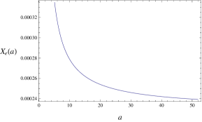
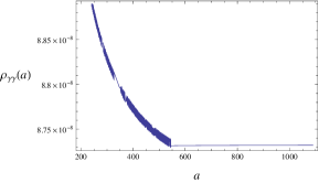
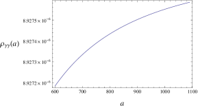
With the these parameters equation (78) was solved numerically. Some values of the ionization fraction as a function of the scale factor are presented in Table 1 and plots of and are shown in Figure 1. Below we solve numerically equations describing evolution of the mixed graviton-photon density matrix together with equation (78) introducing into them a factor describing reionization of the cosmic plasma.
| 1 | |
| 1.04 | |
| 1.18 | |
| 1.23 | |
| 1.5 | |
| 2 | |
| 4 | |
| 10 | |
| 30 | |
| 51.9 | |
| 136.25 | |
| 1090 | 1 |
.

The resonance condition, , is fulfilled at
| (83) |
The ratio of the oscillation length to the mean free path in this case is
| (84) |
In this case the resonance frequency at recombination would be about 10 MeV for G. For possibly larger resonance shifts to smaller . Even out of the resonance inequality may remain true and use of the density matrix formalism is obligatory.
We need to mention however, that very energetic gravitational waves with energy would create photons whose scattering on electrons is weaker than the Thompson one, roughly speaking, by . This effect would diminish the damping factor by the same amount and can be easily taken into account. One has however to keep in mind that the Heisenberg-Euler approximation is valid only for and thus we should not go beyond that value.
In the process of the cosmological expansion the graviton-photon transition could pass through resonance if their frequency satisfies resonance condition (83). However, since we consider graviton energies, , the resonance condition (83) is not satisfied in the post-recombination epoch.
Next we need to evaluate factor . Since, we are interested in the cosmological epoch just after recombination till the present time, when the Universe is dominated by nonrelativistic matter, the Hubble constant as a function of the redshift is given by equation (59). In terms of the scale factor, the product is given by
| (85) |
For redshift we can neglect the contribution of the cosmological constant into the energy density of the Universe since it becomes important only for . We take and cm for the former case and cm for the latter case. According to our notations the redshift corresponds to the scale factor with respect to the recombination time.
For the universe is re-ionized by the first generation stars. According to ref. [31] if the universe went into a sudden complete ionization, the re-ionization redshift is excluded at 99% (CL) in favor of . Using the WMAP 5 year data the authors of ref. [31] suggest that the universe underwent an extended period of partial re-ionization starting at and ending with a complete ionization for instead of a sudden re-ionization. For the value of the scale factor with respect to recombination is and for , .
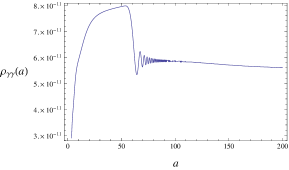
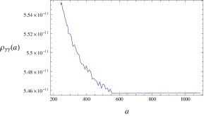
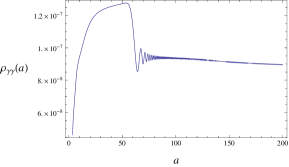
In Fig. 2, Fig. 3, and Fig. 4 the probability of photon creation, is presented as a function of the cosmological scale factor for various values of the initial background magnetic field and for graviton energy eV. For such , the resonance does not occur but still the probability is much higher than the simple estimate in the wave function formalism. We can see that in all Fig. 2, Fig. 3, and Fig. 4 the oscillation probability rapidly increases for and remains almost constant for until onset of the period of reionization at . The rapid increase of for is due to two reasons: a quick drop of the ionization fraction from its value at recombination and sharp decrease of the oscillation frequency. For the ionization fraction practically remains constant with slowly rising. From beginning of the reionization period at till or , slowly decreases with superimposed oscillations of decreasing amplitude. For the vacuum energy density dominates over the matter energy density. At this period the photon creation probability remains almost constant. The oscillation probability drops from up to roughly speaking by 20-30 %. The value of the magnetic field at recombination has been evaluated by the anti-redshift of the present day large scale magnetic field as given in ref. [17, 18].

6 Models of an early production of high frequency gravitons.
In the previous section we calculated the probability of graviton-to-photon transition taking into account both redshift and coherence breaking in plasma and found that for graviton energy of the order of MeV the oscillation probability is quite large, for G up to for G. The number density of the produced photons, which could be directly observed as X-ray background, is proportional to the initial density of the gravitons. The amount of GWs at present time is usually expressed through the density parameter in gravitational waves which is defined as
| (86) |
where is the present day critical energy density:
| (87) |
is the present day GW frequency and is the universe age. Since we are interested in GWs of cosmological origin, we consider here only those emitted before BBN.
The abundances of light elements produced at BBN depend upon the energy density of relativistic species at sec, see e.g. book [32]. According to the recent data [33] an additional energy density at BBN, equal to that of one massless neutrino is allowed and even desirable, . The particles which carry this additional energy are not known. They are called generically dark radiation. At BBN the energy density of one neutrino species (that is of neutrino plus antineutrino with vanishing chemical potential) is approximately equal to that of photons. However after -annihilation the ratio of neutrino to photons energy densities dropped down approximately by factor four. Keeping in mind that the contemporary energy density of CMB photons is , we find that the total energy density of the gravitational waves integrated over their spectrum in the present day universe cannot exceed
| (88) |
where is the allowed by BBN number of the effective neutrino species. Equation (88) is an absolute bound on the energy density of all GWs produced before BBN. It would be interesting if is explained by primordial GWs.
The oscillation probability strongly depends on the graviton frequency and spectrum. The models of primordial GW production mostly predict low frequency of stochastic background of GWs, mainly concentrated at the present day frequencies of GWs near Hz. For example, inflationary models predict an almost scale invariant spectrum at large wavelengths, and their density parameter depends mainly on two factors, the GW frequency and the Hubble parameter at inflation. In the frequency range Hz up to GHz the density parameter is very low, . Other post inflationary models such as pre-heating phase [34], first order phase transitions [35], and topological defects [36], in particular, cosmic strings [37] predict in the high frequency range GHz the density parameter of the order .
All the above mentioned GWs production models, though predict a substantial density parameter, have maximum frequency today not more than eV. We calculated numerically the graviton-photon oscillation probability for frequencies eV and found that it is of the order, . With this low value of the probability the total density parameter in photons of most of post-inflationary GWs models at the maximum frequency GHz would be
| (89) |
Such a small value of the density parameter makes improbable observations of photons from these GWs.
However there is a particular model of GWs emission during the cosmological time interval between the Big Bang and the BBN epoch which leads to rather high cosmological energy density of the very energetic GWs. It was suggested in ref. [7, 38] that after Big Bang the Universe could have passed a transient stage of matter domination by very light primordial black holes of mass g, which would completely evaporate before BBN leaving no trace. The number density of such light BHs is not constrained by any observational data and during their domination it could reach value of the order of unity. In particular, in ref. [7] different mechanisms of GWs emission are considered, where the produced amount of GW could exceed that produced by other mechanisms. Among the mechanisms considered there, we single out the graviton evaporation, where the emitted peak frequency of quasi-thermal gravitons would be in the range from keV up to MeV today. The peak frequency in this model depends on the BH mass which turns out to be in the interval from the Planck mass, up to g.
Let us consider, for example, gravitons with the initial energy eV. Their frequency today would be eV and they would produce photons with the same frequency. The value of the graviton density parameter at this frequency according to the above quoted scenario, could be . And so the corresponding density parameter of the produced photons could be in the interval(or even two orders of magnitude higher):
| (90) |
where is the probability of graviton to photon conversion. The energy flux of such photon background at the present time would be
| (91) |
where is the 00 component of the GW energy-momentum tensor and we restored the light velocity in order to express the photon flux in the standard units (erg/cm2 s). Taking the present day photon energy keV, cm/s and gr/cm-3 we obtain the energy flux
| (92) |
which is comparable to the energy flux of most AGNs in the soft X-ray spectrum [39] and even higher.
7 Discussion and conclusion
We have shown that the probability of the graviton-to-photon transition in large scale cosmological magnetic field after recombination epoch could be in the range at frequencies in 0.1 keV range (in the present day values). An efficient oscillations between graviton and photon could exist at higher frequencies too, but the Heisenberg-Euler approximation, which we use in this work, becomes invalid at energies exceeding the electron mass. This will be considered elsewhere.
For smaller frequencies, e.g. 1 eV, the transition probability would be smaller, by about 2-3 orders of magnitude. The oscillation probability strongly depends on the external magnetic field and the graviton energy. For higher values of these parameters, as our numerical calculations show, the oscillation probability can increase by several orders of magnitude.
The photons produced by such mechanism could make considerable contribution to cosmic electromagnetic background if the density of the original gravitational waves, , is sufficiently high. We have estimated efficiency of the photon production in various models of primordial GW generation discussed in the literature. Mostly, in the considered inflationary and post-inflationary models the density of photons produced by the GWs is quite low and is not observable at the present time.
The mechanism discussed here gives a large number of photons (for fixed values of the magnetic field) only for high frequency gravitons. We think that given the present GWs production models the only mechanism before BBN that could generate a measurable flux of photons is the graviton production by primordial black holes. Since PBH emit thermal gravitons (if one neglects gray body corrections) the spectrum of the GWs today would be rather close to the original one with some distortion induced by the different cosmological moments of GW creation, as shown in the first paper of ref. [7].
After hydrogen recombination the plasma density drops down
and the interaction of the photons, created by the graviton-photon transition,
with electrons becomes much weaker in complete analogy with the CMB photons. Such photons could make
observable contributions to the cosmological electromagnetic background, in particular, to X-rays or extragalactic
light. If we consider a conservative present day density parameter , the energy flux in X-rays by the proposed mechanism would be of the order erg/cm2/s where the flux upper limit is 10 percent less than the observed energy flux in the soft X-rays [40]. If we assume that the total density of the gravitational waves reaches its upper bound allowed by BBN (and explains
the possibly observed dark radiation),
, and that their frequency is close to 0.1 keV, the energy flux today would be in the range, erg/cm2/s. This energy flux could explain the cosmic X-ray background being its dominant part without requiring any obscured AGN.
Acknowledgements A. Dolgov acknowledges the support of the Russian Federation Government Grant No. 11.G34.31.0047. D. Ejlli thanks D. Semikoz for useful discussions on the present limits of the large scale magnetic fields and the spectrum of extragalactic radiation.
References
- [1] A. Einstein, Sitzungsber. Preuss. Akad. Wiss. Berlin (Math. Phys. ) 1916 (1918) 154.
- [2] R. A. Hulse, J. H. Taylor, Astrophys. J. 195 (1975) L51-L53.
-
[3]
B.S. Sathyaprakash, B.F. Schutz, Living Rev.Rel. 12 (2009) 2
arXiv:0903.0338 [gr-qc].
K. Riles, arXiv:1209.0667 [hep-ex].
M. Maggiore, Phys. Rept. 331 (2000) 283 [gr-qc/9909001]. - [4] L. P. Grishchuk, Sov. Phys. JETP 40 (1975) 409.
- [5] A. A. Starobinsky, JETP Lett. 30 (1979) 682.
- [6] V. A. Rubakov, M. V. Sazhin, A. V. Veryaskin, Phys. Lett. B115 (1982) 189.
-
[7]
A. D. Dolgov and D. Ejlli,
Phys. Rev. D 84 (2011) 024028
[arXiv:1105.2303 [astro-ph.CO]].
A.D. Dolgov, P.D. Naselsky, I.D. Novikov, astro-ph/0009407. - [8] M.E. Gertsenshtein, ZhETF 41 (1961) 113 [Sov. Phys. JETP, 14 (1961) 84].
-
[9]
N.V. Mitskevich, Fizicheskie polya v obschej teorii otnositel’nosti (Physical fields in General
Relativity), Nauka, Moscow, 1970;
D. Boccaletti, V. De Sabbata, P. Fortini, C. Gualdi, Nuovo Cimento, 70B (1970) 129;
V.K.Dubrovich, Izv. Spet. Astro. Obs. 6 (1972) 27;
Ya.B. Zel’dovich, Zh. Eksp. Teor. Fiz. 65 (1973) 1311 [Sov. Phys. JETP, 38 (1974) 652.
D. Fargion, Gravitation and Cosmology, 1 (1995) 301-310 - [10] G. Raffelt and L. Stodolsky, Phys. Rev. D 37 (1988) 1237.
-
[11]
W. Heisenberg, H. Euler, Z. Phys. 98 (1936) 714.
J. S. Schwinger, Phys. Rev. 82 (1951) 664. - [12] C. W. Misner, K. S. Thorne and J. A. Wheeler, San Francisco 1973, 1279p
-
[13]
E. Brezin and C. Itzykson,
Phys. Rev. D 3 (1971) 618.
S. L. Adler, Annals Phys. 67 (1971) 599. - [14] C. Giunti and C. W. Kim, Oxford, UK: Univ. Pr. (2007) 710 p
- [15] R. Durrer, P. G. Ferreira and T. Kahniashvili, Phys. Rev. D 61 (2000) 043001 [astro-ph/9911040].
- [16] J. D. Barrow, P. G. Ferreira and J. Silk, Phys. Rev. Lett. 78 (1997) 3610 [astro-ph/9701063].
-
[17]
D. Paoletti and F. Finelli,
arXiv:1208.2625 [astro-ph.CO].
D. Paoletti and F. Finelli, Phys. Rev. D 83 (2011) 123533 [arXiv:1005.0148 [astro-ph.CO]].
D. Paoletti, F. Finelli and F. Paci, Mon. Not. Roy. Astron. Soc. 396 (2009) 523 [arXiv:0811.0230 [astro-ph]]. -
[18]
T. Kahniashvili, Y. Maravin and A. Kosowsky,
Phys. Rev. D 80 (2009) 023009
[arXiv:0806.1876 [astro-ph]].
- [19] C. Caprini and R. Durrer, Phys. Rev. D 65 (2001) 023517 [astro-ph/0106244]. C. Caprini and R. Durrer, Phys. Rev. D 72 (2005) 088301 [astro-ph/0504553].
- [20] A. Kosowsky, T. Kahniashvili, G. Lavrelashvili and B. Ratra, Phys. Rev. D 71 (2005) 043006 [astro-ph/0409767].
- [21] E. Komatsu et al. [WMAP Collaboration], Astrophys. J. Suppl. 192 (2011) 18 [arXiv:1001.4538 [astro-ph.CO]].
-
[22]
M. Giovannini,
Int. J. Mod. Phys. D 13 (2004) 391
[astro-ph/0312614].
D. Grasso and H. R. Rubinstein, Phys. Rept. 348 (2001) 163 [astro-ph/0009061]. -
[23]
J. J. Matese and R. F. O’Connell,
Phys. Rev. 180 (1969) 1289.
R. F. O’Connell and J. J. Matese, Nature 222 (1969) 649-650.
G. Greenstein, Nature 223 (1969) 938-939 -
[24]
P. J. Kernan, G. D. Starkman and T. Vachaspati,
Phys. Rev. D 56 (1997) 3766
[astro-ph/9612101].
B. Cheng, A. V. Olinto, D. N. Schramm and J. W. Truran, Phys. Rev. D 54 (1996) 4714 [astro-ph/9606163].
P. J. Kernan, G. D. Starkman and T. Vachaspati, Phys. Rev. D 54 (1996) 7207 [astro-ph/9509126]
D. Grasso and H. R. Rubinstein, Astropart. Phys. 3 (1995) 95 [astro-ph/9409010]. -
[25]
N. A. Zabotin and P. D. Naselskii, Soviet Astronomy, v. 26, p. 272, (1982).
B. J. T. Jones and R. F. G. Wyse, A&A 1985, 149, 144-150 - [26] M. S. Pshirkov and D. Baskaran, Phys. Rev. D 80 (2009) 042002 [arXiv:0903.4160 [gr-qc]].
- [27] A.D. Dolgov, Yad. Fiz. 33 (1981) 1309 (in Russian); Sov. J. Nucl. Phys. 33 (1981) 700.
-
[28]
G. Sigl, G. Raffelt, Nucl. Phys. B 406 (1993) 423;
A.D. Dolgov, Phys. Repts. 370 (2002) 333. - [29] S. Weinberg, “Cosmology,” Oxford, UK: Oxford Univ. Pr. (2008) 593 p
-
[30]
D. G. Hummer,
Mon. Not. Roy. Astron. Soc. 268 (1994) 109.
D. Péquignot, P. Petijan and C. Boisson, Astron. Astrophys. 251 (1991) 680. - [31] J. Dunkley et al. [WMAP Collaboration], Astrophys. J. Suppl. 180 (2009) 306 [arXiv:0803.0586 [astro-ph]].
- [32] E. W. Kolb and M. S. Turner, “The Early universe,” Front. Phys. 69 (1990) 1.
- [33] For a recent review see e.g. A. Coc, Invited Plenary Talk given at the 11th International Conference on Nucleus-Nucleus Collisions (NN2012), San Antonio, Texas, USA, May 27-June 1, 2012. To appear in the NN2012 Proceedings in Journal of Physics: Conference Series (JPCS), arXiv:1208.4748.
- [34] R. Easther, E. A. Lim, JCAP 0604 (2006) 010. [astro-ph/0601617]. R. Easther, J. T. Giblin, E. A. Lim, Phys. Rev. D77 (2008) 103519. [arXiv:0712.2991]
- [35] C. Grojean, G. Servant, Phys. Rev. D75 (2007) 043507. [hep-ph/0607107]
- [36] A. Mazumdar, I. M. Shoemaker, [arXiv:1010.1546].
- [37] C. J. Hogan, Phys. Rev. D74 (2006) 043526. [astro-ph/0605567]. M. R. DePies, C. J. Hogan, Phys. Rev. D75 (2007) 125006. [astro-ph/0702335]
- [38] R. Anantua, R. Easther and J. T. Giblin, Phys. Rev. Lett. 103 (2009) 111303 [arXiv:0812.0825 [astro-ph]].
- [39] Lehman et al. 2001 A&A 371 833L; Akiyama et al. 2000 ApJ 532 700A
-
[40]
M. Ajello, J. Greiner, G. Sato, D. R. Willis, G. Kanbach, A. W. Strong, R. Diehl and G. Hasinger et al.,
arXiv:0808.3377 [astro-ph].
G. Hasinger [CDF-S Team Collaboration], AIP Conf. Proc. 666 (2003) 227 [astro-ph/0302574].
Hasinger, G., Burg, R., Giacconi, R., et al., 1998, A&A 329, 482