The universality class of the continuous phase transition in the $2D$ “Touch and Stop” cluster growth percolation model

Abstract

We consider the “Touch and Stop” cluster growth percolation (CGP) model on the two dimensional square lattice. A key-parameter in the model is the fraction $p$ of occupied “seed” sites that act as nucleation centers from which a particular cluster growth procedure is started. Here, we consider two growth-styles: rhombic and disk-shaped cluster growth. For intermediate values of $p$ the final state, attained by the growth procedure, exhibits a cluster of occupied sites that spans the entire lattice. Using numerical simulations we investigate the percolation probability and the order parameter and perform a finite-size scaling analysis for lattices of side length up to $L\!=\!1024$ in order to carefully determine the critical exponents that govern the respective transition. In contrast to previous studies, reported in [Tsakiris et al., Phys. Rev. E 82 (2010) 041108], we find strong numerical evidence that the CGP model is in the standard percolation universality class.

I Introduction

The pivotal question in standard percolation Stauffer (1979); Stauffer and Aharony (1994) is that of connectivity. A basic example is $2D$ random site percolation, where one studies a lattice in which a random fraction $p$ of the sites is “occupied”. Clusters composed of adjacent occupied sites are then analyzed regarding their geometric properties. Depending on the fraction $p$ of occupied sites, the geometric properties of the clusters change, leading from a phase with rather small and disconnected clusters to a phase, where there is basically one large cluster covering the lattice. Therein, the appearance of an infinite, i.e. percolating, cluster is described by a second-order phase transition.

There is a wealth of literature on a multitude of variants on the above basic percolation problem that model all kinds of phenomena, ranging from simple configurational statistics to “string”-bearing models that also involve a high degree of optimization, e.g. describing vortices in high $T_{c}$ superconductivity Pfeiffer and Rieger (2002, 2003) and domain wall excitations in disordered media such as $2D$ spin glasses Cieplak et al. (1994); Melchert and Hartmann (2007) and the $2D$ solid-on-solid model Schwarz et al. (2009). Besides discrete lattice models there is also interest in studying continuum percolation models, where recent studies reported on highly precise estimates of critical properties for spatially extended, randomly oriented and possibly overlapping objects with various shapes Mertens and Moore (2012).

One such variant of the above basic percolation model is the recently proposed “Touch and Stop” cluster growth percolation (CGP) model Tsakiris et al. (2010a, b). In the CGP model, a random fraction of $p$ sites is distinguished to comprise a set of “seed” sites for which a particular cluster growth procedure is evolved (see sect. II). I.e., starting from the seed sites, clusters are grown by assimilating all nearest neighbor sites layer by layer in an iterative, discrete time fashion. As soon as one cluster comes in contact with other clusters, the growth procedure for all involved clusters is stopped. When there is no growing cluster left, the cluster growth procedure is completed and the connected regions of adjacent occupied sites, i.e. the final clusters, are analyzed regarding their geometric properties. To support intuition: if $p$ is rather small, the growth of a particular cluster is unlikely to be hindered by other clusters within the first few time steps, since the typical distance between the respective seed sites is large compared to the lattice spacing. Consequently, the final clusters are rather large, see Fig. 1(a). As $p$ increases, the typical size of clusters in the final configuration decreases due to the increasing density of initial seed sites, see Figs. 1(a–c). Increasing $p$ even further leads to an increasing size of the largest cluster. This is due to the larger probability to yield adjacent seed sites already in the initial configuration, for which a growth procedure is subsequently inhibited. For increasing $p$ and due to spacial homogeneity this in turn leads to an increase of the size of the largest cluster, see Figs. 1(c–e).

The two distinct scaling regimes of the largest cluster size were discussed in Ref. Tsakiris et al. (2010a). The behavior at small values of $p$ was illustrated to be a finite size effect and the scaling at intermediate values of $p$ was found to signal a continuous phase transition qualitatively similar to the standard percolation transition. In Ref. Tsakiris et al. (2010b), the critical properties of the latter transition were addressed. Albeit the authors of Ref. Tsakiris et al. (2010b) perform a scaling analysis to estimate the critical point and a set of critical exponents that govern the phase transition, we are convinced that the analysis can be improved in various ways. In this regard, we here revisit the continuous phase transition found for the CGP model at intermediate values of $p$ and perform a finite size scaling analysis considering geometric properties of the largest cluster for the individual final configurations obtained using computer simulations. To this end, the results we report in sect. III below (obtained using two different cluster growth styles, i.e. rhombic and disk-shaped cluster growth) are different from those presented in Ref. Tsakiris et al. (2010b) in the following respect: in contrast to their findings we here present strong numerical evidence that the percolation transition of the CGP model at intermediate values of $p$ is in the same universality class as standard percolation. By employing the data collapse technique for different observables we aim to yield maximally justifiable results due to a high degree of numerical redundancy. Further, we analyze the distribution of cluster sizes right at the critical point in order to numerically assess a particular critical exponent that was previously only computed via scaling relations.

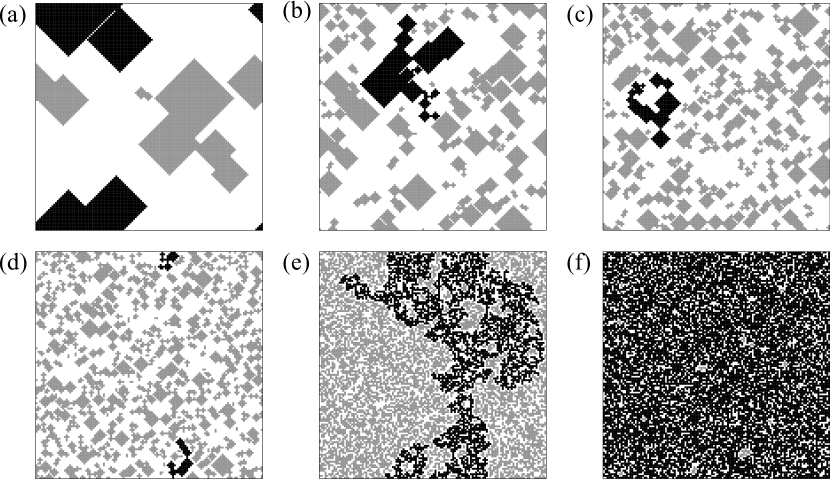
Figure 1: Samples of final configurations obtained for the CGP model on $2D$ square lattices of side length $L\!=\!128$. The snapshots relate to different values of the initial density of active seed sites: $p\!=\!0.001$, $0.01$, $0.02$, $0.05$, $0.495$, $0.7$, for subfigures (a–f), respectively. In the limit of large system sizes and above the critical point $p_{c}\approx 0.495$, the largest cluster in the final configuration spans the lattice along at least one direction. In each subfigure, the largest cluster is colored black and all finite clusters are colored grey.

The remainder of the presented article is organized as follows. In section II, we introduce the model in more detail. In section III, we outline the data collapse technique and we list the results of our numerical simulations. Therein, the discussion is focused on rhombic cluster growth. Section IV concludes with a summary. Appendix A shows a further analysis of the order parameter resembling the one presented in Ref. Tsakiris et al. (2010b), and appendix B elaborates on the results obtained for disk-shaped cluster growth.

II Model and Algorithm

Here, we consider $2D$ square lattices of side length $L$ and $N=L^{2}$ sites. Initially, a starting configuration is prepared by occupying a random fraction $p$ of the lattice sites via seed sites. These seeds indicate the centers of a set of active clusters that will evolve during the growth procedure. The remaining sites are considered empty. For the set of active clusters, the growth procedure consists of the repeated application of the following two steps: (i) to perform a single sweep, consider the still active clusters sequentially in random order. For each cluster perform the cluster update below. (ii) so as to perform a single cluster update, consider the surface of the respective cluster, i.e. the set of nearest neighbor sites of those sites that build up the current cluster and that do not belong to the cluster, yet. To complete a cluster update, the “Touch and Stop” CGP model discriminates the following two situations: (ii.1) if alien sites, i.e. sites belonging to clusters different from the current one are found among the surface sites, the cluster growth procedure for all involved clusters is stopped. The respective clusters are further deleted from the set of active clusters; (ii.2) if all surface sites are empty, amend the current cluster by the set of surface sites. The above two steps (i) and (ii) are iterated until no active cluster is left and the final configuration is reached. I.e., the evolution of the system proceeds in discrete time-steps, where within one particular time-step each active cluster is updated once. Note that the precise configuration of occupied sites in the final configuration might depend on the order in which active clusters are picked in step (i).

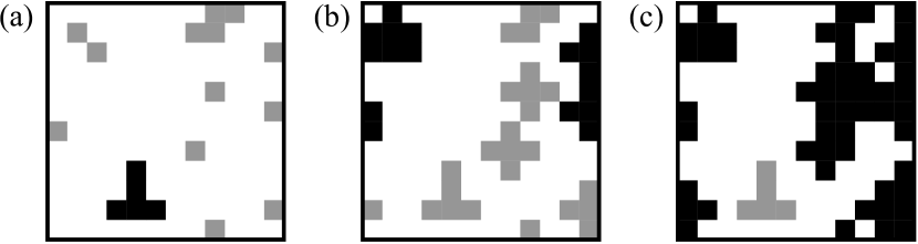
Figure 2: Example of the cluster growth procedure for a $2D$ square lattice of side length $L\!=\!12$. For the initial configuration of active seed sites shown in subfigure (a), the growth procedure is completed after the two steps (a–b) and (b–c), already. Subfigure (c) indicates the final configuration. See text for more details.

Fig. 2 illustrates the cluster growth procedure for a square lattice of side length $L=12$, where initially $18$ seed sites are present (see Fig. 2(a)), i.e. $p=0.125$. The $18$ seed sites are arranged in $10$ clusters. Consequently, the initial configuration exhibits small clusters of adjacent occupied sites for which, according to step (ii) above, not a single cluster update is performed. Both of these clusters occupy $5$ sites and one of them is picked to signify the largest cluster on the lattice. In the figure it is colored black to distinguish it from the other clusters (which are colored grey). While sweeping over the active clusters in step (i), a successful cluster update for one cluster might hinder the growth of another cluster that still has to be considered in the respective sweep (see, e.g., the two occupied next nearest neighbor sites in the upper left corner of Fig. 2(a)). After one sweep the configuration of occupied clusters has changed, see Fig. 2(b). Now, the largest cluster comprises $15$ sites and there are only three active clusters left. The next sweep, resulting in the final configuration shown in Fig. 2(c), completes the growth procedure. Therein, the largest cluster occupies $53$ sites and it spans the lattice along the vertical direction since its projection on the independent lattice axis covers $12$ sites in the vertical direction.

As pointed out in the introduction and discussed in Ref. Tsakiris et al. (2010a), the model features two transitions: a sharp transition at a very small value of $p$, which is due to finite size effects, and a continuous transition at intermediate values of $p$. Below, we will perform simulations on square systems of finite size and for different values of $p$ in order to assess the critical properties of the CGP model in the vicinity of the critical point in $2D$. The observables we consider are derived from the set of clusters in the final configuration, attained after the growth process is completed. The observables will be introduced and discussed in the subsequent section.

III Results

So as to assess the critical properties of the CGP model in the vicinity of the critical point in $2D$ we performed simulations for square lattices of side length up to $L=1024$. For each system size considered, we recorded data sets at $24$ supporting points in a $p$-range that encloses the critical point on the $p$-axis. Each data set comprises the set of clusters in the final configuration for $\approx 10^{4}$ individual samples. As stressed in the introduction, we consider two different cluster growth styles: rhombic and disk-shaped cluster growth, defining the rhombic CGP model (CGP-R) and the disk-shaped CGP model (CGP-D), respectively. In the remainder of this section we report on the results for rhombic cluster growth. The results for disk-shaped cluster growth are detailed in appendix B.

Most of the observables we consider below can be rescaled following a common scaling assumption (formulated below for a general observable $y(p,L)$). This scaling assumption states that if the observable obeys scaling, it can be expressed as

$$y(p,L)=L^{-b}~{}f[(p-p_{c})L^{a}],$$ (1)

wherein $a$ and $b$ represent dimensionless critical exponents (or ratios thereof, see below), $p_{c}$ signifies the critical point, and $f[\cdot]$ denotes an unknown scaling function. Following Eq. (1), data curves of the observable $y(p,L)$ recorded at different values of $p$ and $L$ collapse, i.e. fall on top of each other, if $y(p,L)L^{b}$ is plotted against the combined quantity $\epsilon\equiv(p-p_{c})L^{a}$ and if the scaling parameters $p_{c}$, $a$ and $b$ that enter Eq. (1) are chosen properly. The values of the scaling parameters that yield the best data collapse signify the numerical values of the critical exponents that govern the scaling behavior of the underlying observable $y(p,L)$. In order to obtain a data collapse for a given set of data curves we here perform a computer assisted scaling analysis, see Refs. Houdayer and Hartmann (2004); Melchert (2009). The resulting numerical estimates of the critical point and the critical exponents for the $2D$ “Touch and Stop” model implemented using rhombic and disk-shaped cluster growth as well as the critical properties of the standard $2D$ site percolation model (for comparison) are listed in Tab. 1. Below, we report on the results found for different observables:

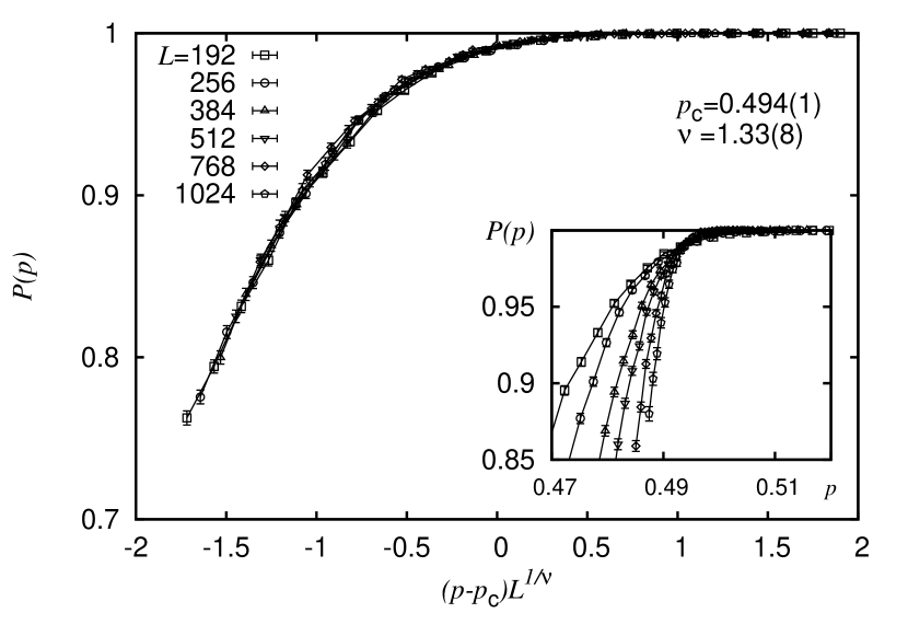
Figure 3: Finite size scaling of the spanning probability $P(p)$ for the CGP-R model on $2D$ square lattice of side length $L=192$ through $1024$, averaged over different initial seed configurations. The main plot shows the data collapse obtained according to Eq. 1, and the inset illustrates the raw data close to the critical point.

Table 1: Critical properties that characterize the CGP phenomenon (CGP-R: rhombic clusters; CGP-D: disk-shaped clusters) in $2D$. From left to right: Critical point $p_{c}$, critical exponents $\nu$, $\beta$, $\gamma$, and $\tau$. For comparison, the critical properties for the standard site percolation (SP) problem on the $2D$ square lattice (figures up to the third decimal) are listed also.

	$p_{c}$	$\nu$	$\beta$	$\gamma$	$\tau$
CGP-R	0.4938(7)	1.33(3)	0.141(3)	2.38(5)	2.057(1)
CGP-D	0.4978(5)	1.32(4)	0.145(4)	2.38(3)	2.050(6)
SP	0.593	$1.333$	$0.139$	$2.389$	$2.055$

Spanning probability:

As a first observable we consider the probability $P(p)$ that the final configuration features a cluster that spans the lattice along at least one direction, averaged over different initial seed configurations. It is expected to scale according to Eq. (1), where $a=1/\nu$ and $b=0$. A data collapse performed for the four largest system sizes $L=384,512,768,1024$ in the range $\epsilon\in[-2,2]$ on the rescaled $p$-axis yields the scaling parameters $p_{c}=0.494(1)$, and $\nu=1.34(7)$ for a quality $S=0.71$ of the data collapse, see Fig. 3. As it appears, the numerical value of $\nu$ agrees well with the value for standard $2D$ percolation, i.e. $\nu_{\rm perc}=4/3$. While the location of the critical point is in agreement with the value reported in Ref. Tsakiris et al. (2010b), the critical exponent is rather different (Ref. Tsakiris et al. (2010b) reports $\nu=1.17$).

Order parameter:

As a second observable we consider the order parameter, given by the relative size

$$P_{\rm max}(p)=\langle s_{\rm max}(p)\rangle$$ (2)

of the largest cluster in the final configuration, averaged over different initial seed configurations. This observable scales according to Eq. (1), where $a=1/\nu$ and $b=-\beta/\nu$. Again, a data collapse for the four largest system sizes in the range $\epsilon\in[-2,2]$ yields the scaling parameters $p_{c}=0.4937(2)$, $\nu=1.34(5)$, and $\beta=0.141(3)$ for a quality $S=0.77$ of the data collapse, see Fig. 4(b). Note that the numerical value of the order parameter exponent $\beta$ is in agreement with the standard percolation exponent $\beta_{\rm perc}=5/36\approx 0.139$ (Ref. Tsakiris et al. (2010b) reports $\beta=0.24$).

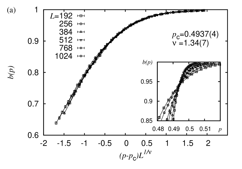
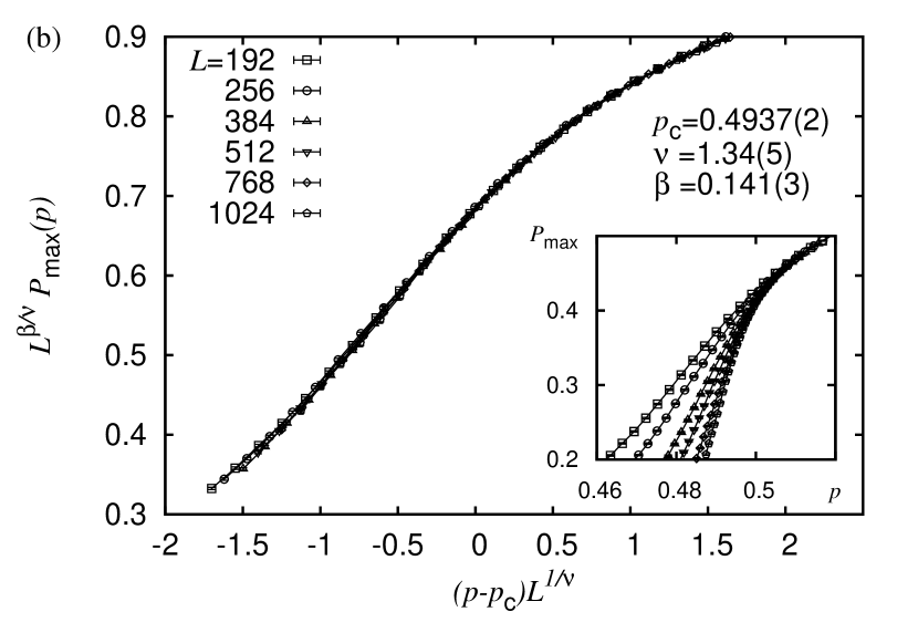
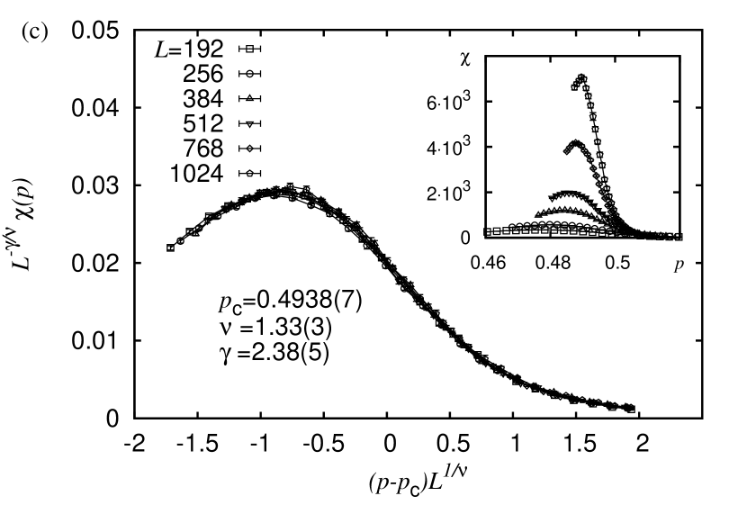
Figure 4: Finite size scaling analyses related to the relative size $s_{\rm max}$ of the largest cluster for the CGP-R model on $2D$ square lattice of side length $L=192$ through $1024$, averaged over different initial seed configurations. The main plots show the data collapse obtained according to Eq. 1, and the insets illustrate the raw data close to the critical point. The subfigures show different ways to analyze $s_{\rm max}$ in terms of (a) the Binder parameter $b(p)$, (b) the order parameter $s_{\rm max}(p)$ itself, and, (c) the fluctuation $\chi(p)=N{\rm var}(s_{\rm max})$ of the order parameter.

A different way to analyze the same set of data is in terms of the Binder ratio Binder (1981)

$$b(p)=\frac{1}{2}\Big{[}3-\frac{\langle s_{\rm max}^{4}(p)\rangle}{\langle s_{\rm max}^{2}(p)\rangle^{2}}\Big{]}.$$ (3)

This observable scales according to Eq. (1), where, as for the spanning probability above, $a=1/\nu$ and $b=0$. The best data collapse yields $p_{c}=0.4937(4)$, and $\nu=1.34(8)$ with a quality $S=0.96$ in the range $\epsilon\in[-2,2]$, see Fig. 4(a).

A further critical exponent can be estimated from the scaling of the order parameter fluctuations $\chi(p)$, defined as

$$\chi(p)=N[\langle s_{\rm max}^{2}(p)\rangle-\langle s_{\rm max}(p)\rangle^{2}].$$ (4)

The order parameter fluctuations are expected to scale according to Eq. (1), where $a=1/\nu$, and $b=-\gamma/\nu$. A best data collapse is attained for $p_{c}=0.4938(7)$, $\nu=1.33(3)$, and $\gamma=2.38(5)$ with a quality $S=0.84$, again in the range $\epsilon\in[-2,2]$, see Fig. 4(c). Here, the numerical value of the fluctuation exponent $\gamma$ is in agreement with the standard percolation exponent $\gamma_{\rm perc}=43/18\approx 2.389$ (Ref. Tsakiris et al. (2010b) reports $\gamma=1.91$).

Average size of the finite clusters:

As a third observable we consider the average size $\langle S_{\rm fin}(p)\rangle$ of all finite clusters for a particular final configuration, averaged over different initial seed configurations Sur et al. (1976); Stauffer and Aharony (1994). This observable is defined as

$$S_{\rm fin}(p)=\frac{\sum_{s}^{\prime}s^{2}\,n_{s}(p)}{\sum_{s}^{\prime}s\,n_{s}(p)},$$ (5)

where $n_{s}(p)$ indicates the probability mass function of cluster sizes for a single sample at a given value of $p$. Note that the sums run over finite clusters only Sur et al. (1976); Stauffer and Aharony (1994) (indicated by the prime), i.e. if a final configuration features a system spanning cluster, this cluster is excluded from the sums. The average size of all finite clusters is expected to scale according to Eq. (1), where $a=1/\nu$ and $b=-\gamma/\nu$. For this observable, considering the system sizes $L=128,192,256,384$, a best data collapse is found for $p_{c}=0.491(1)$, $\nu=1.35(2)$, and $\gamma=2.37(3)$ with a quality $S=1.81$ of the data collapse. Considering the sequence of larger system sizes $L=384,512,768,1024$, the optimal choices for the scaling parameters result in $p_{c}=0.4930(5)$, $\nu=1.35(2)$, and $\gamma=2.35(4)$ with a quality $S=1.16$. Both results agree within errorbars and were obtained in the range $\epsilon\in[-1,1]$. Further, the value of $\gamma$ estimated from the average size of the finite clusters support the numerical value estimated from the scaling behavior of the order parameter fluctuations.

Further observables recorded at $p_{c}$:

The various estimates for the critical point are in agreement with $p_{c}=0.494(1)$. At this critical point, Eq. (1) reduces to $y(p_{c},L)\propto L^{-b}$. We performed additional simulations at $p_{c}$ to determine the scaling dimension of the largest cluster $S_{\rm max}$, defining the fractal dimension $d_{f}$ according to $\langle S_{\rm max}\rangle\propto L^{d_{f}}$. Considering the scaling form $\langle S_{\rm max}\rangle(L)=aL^{d_{f}}$ for a fit in the interval $L\in[20,1024]$, we find $a=0.669(1)$, and $d_{f}=1.8995(4)$ (where the reduced $\chi^{2}$-value reads $\chi^{2}_{\rm red}=0.65$), see inset of Fig. 5. Albeit the error bars obtained from the least-squares fit is notoriously small, the numerical value of the fractal dimension itself is in good agreement with the ordinary percolation estimate $d_{f,{\rm perc}}=91/48\approx 1.896$ (Ref. Tsakiris et al. (2010b) report $d_{f}=1.79(1)$).

Figure 5: Scaling analysis of different observables at the critical point $p_{c}$ of the CGP-R model. The main plot shows the probability mass function $n_{s}$ of clusters of size $s$, displayed using logarithmic binning. The inset illustrates the scaling of the average size $\langle S_{\rm max}\rangle$ of the largest cluster and the order parameter fluctuations $\chi$.

For numerical redundancy we further estimate the exponent ratio $\gamma/\nu$ from the order parameter fluctuations, Eq. (4), at $p_{c}$ via $\chi(L)\propto L^{\gamma/\nu}$, where a fit to the interval $L\in[20,1024]$ yields $\gamma/\nu=1.772(3)$ ($\chi^{2}_{\rm red}=1.0$). Allowing for a slight deviation from the pure power law form using the effective scaling form $\chi(L)\propto(L+\Delta L)^{\gamma/\nu}$, we obtain $\gamma/\nu=1.785(8)$ ($\chi^{2}_{\rm red}=0.81$), see inset of Fig. 5. Note that the resulting exponent ratio is not only in good agreement with the numerical values for $\gamma$ and $\nu$ obtained above, but also with the standard percolation estimate $\gamma_{\rm perc}/\nu_{\rm perc}=129/72\approx 1.792$ (Ref. Tsakiris et al. (2010b) report $\gamma/\nu=1.63(1)$).

Further, at the critical point we recorded the probability mass function $n_{s}$ for clusters of size $s$. It exhibits an algebraic decay following $n_{s}\propto s^{-\tau}$, for which we estimate the exponent $\tau=2.057(1)$. This estimate was obtained for the data recorded at $L=1024$ using a least-squares fit to the interval $s\in[200,10000]$ (the errorbar was estimate by bootstrap resampling of the underlying datasets), see main plot of Fig. 5. Note that the value is reasonably close to the standard percolation estimate $\tau_{\rm perc}=187/91\approx 2.055$ (Ref. Tsakiris et al. (2010b) report $\tau=2.08$, computed using a hyperscaling relation).

Finally, at $p_{c}$ and on a large lattice of $L=1024$ we estimate the fraction of occupied sites in the final configuration to be $p_{\rm fin}=0.589697(5)$ (for a smaller lattice setup with $L=128$ we find $p_{\rm fin}=0.58964(4)$). These values are only slightly smaller than the fraction $p_{c,{\rm perc}}=0.59274621(13)$ of occupied sites at the critical point of $2D$ site percolation Newman and Ziff (2000); Wikipedia (2012).

IV Conclusions

We have investigated the continuous transition of the “Touch and Stop” cluster growth percolation model at intermediate values of the initial fraction $p$ of seed sites by means of numerical simulations, implementing rhombic and disk-shaped cluster growth. Previously, the critical point and the critical exponents that govern the transition were estimated Tsakiris et al. (2010b) and it was concluded that the transition is in a different universality class than standard percolation. From a point of view of data analysis, the previously presented analysis could be improved in various regards. Here, we have revisited the cluster growth percolation model and performed a finite-size scaling analysis considering the geometric properties of the largest clusters for the individual final configurations attained after the growth procedure is completed. Using large system sizes and appropriate sample sizes, we obtained highly precise estimates for the critical points of both cluster growth styles and the usual critical exponents that characterize the scaling behavior of the spanning probability, the order parameter (and its fluctuations), and the probability mass function of cluster sizes right at the critical point. We further used different observables to estimate individual exponents. E.g., in order to determine the fluctuation exponent $\gamma$, we considered the order parameter fluctuations $\chi$ (using the data collapse techniques shown in Fig. 4(c) as well as the finite-size scaling right at $p_{c}$ illustrated in the inset of Fig. 5) and the average size of the finite clusters $S_{\rm fin}$. This lead to highly redundant numerical estimates for the critical exponents and yields maximally justifiable results.

In summary, we find that the critical exponents estimated for the “Touch and Stop” cluster growth model are in reasonable agreement with those that describe the standard $2D$ percolation phenomenon, see Tab. 1. Hence we conclude that the $2D$ cluster growth percolation model is in the same universality class as standard $2D$ percolation.

Further, we found that in the vicinity of the critical point, the cluster growth procedure (for $L>256$) is completed after $3-4$ steps. I.e., in comparison to ordinary site percolation, the growth procedure can effectively be seen as a process that affects the cluster configurations close to $p_{c}$ only locally. This might render it somewhat intuitive that the cluster growth procedure leads to a shift of the (anyway non-universal) critical point but does not change the critical exponents as compared to standard percolation.

Figure 6: Order parameter analysis for the CGP-R model, similar to that performed by Tsakiris et al. (a) relative size $s_{\rm max}$ of the largest cluster for different system sizes scaled by a factor of $L^{\beta/\nu}$, where $\beta/\nu$ is adjusted such that the data curves exhibit a common crossing point (see text for more details). (b) results of a bootstrap resampling analysis for the analysis in (a). The central figure shows the distribution of tuples $(\beta/\nu,p_{\rm c})$ in the plane and the small adjacent plots show the probability density function along the independent directions. The points with error bars in the central figure show the resulting estimates for the corresponding resampled parameters.

Appendix A Order parameter analysis similar to that of Tsakiris et al.

An admissible criticism of the analysis presented earlier in sect. III is, by considering the order-parameter and using the data-collapse method, one has in principle three parameters ($p_{c}$, $\nu$ and $\beta$) to adjust in order to yield a data collapse. From a practical point of view, one might first consider a dimensionless quantity as, e.g., the percolation probability or the binder ratio, to arrive at estimates for $p_{c}$ and $\nu$ (which are still two parameters to adjust at once). These can then be inserted into the scaling relation for the order-parameter, leaving only the scaling parameter $\beta$ left to adjust in order to obtain a best collapse of the order-parameter curves. We found that whatever protocol we followed, the numerical estimates of the scaling parameters did vary only within their respective errorbars. Hence, from a point of view of analysis using the data-collapse method, the numerical estimates of $p_{c}$, $\nu$, and $\beta$ (as listed in Tab. 1) appear to be consistent and reliable.

However, we also performed an analysis of the order-parameter similar to that of Tsakiris et al., cf. Fig. (4) of Ref. Tsakiris et al. (2010b). The benefit of their “crossing-point” method is that it features only one scaling parameter, namely the exponent ratio $\beta/\nu$ Argyrakis (2012). In the remainder of this appendix we explain the “crossing-point” analysis procedure and report on the results obtained therewith.

Starting with the data curves for the relative size $s_{\rm max}$ of the largest cluster for different system sizes, we scale the data curves by a factor of of $L^{\beta/\nu}$. If we consider $N$ data curves subject to $\beta/\nu>0$, we yield $M=(N(N-1))/2$ presumably different crossing points $p_{i}$, $i=1,\ldots,M$. The exponent ratio $\beta/\nu$ is then adjusted in order to minimize the width $\Delta p={\rm max}(p_{i})-{\rm min}(p_{i})$ of the set of crossing points, resulting in a tuple $(\beta/\nu,p_{\rm c})$ of “optimal” parameters (we set $p_{c}=\sum_{i}p_{i}/M$). In order to estimate errors for these optimal parameters, we performed a bootstrap resampling procedure of the raw data and analyzed each resampled set of data curves using the above procedure. We considered an overall number of $N=6$ data curves and $m=2000$ bootstrap samples. Fig. 6(a) shows one of these bootstrap samples. The analysis of all $m$ optimal tuples $(\beta/\nu,p_{\rm c})$ in the plane is summarized in Fig. 6(b). Therein, the central plot shows the distribution of tuples in the plane and the small adjacent plots show the probability density function along the independent directions. The resulting estimates for the resampled optimal parameters read $\beta/\nu=0.105(11)$ and $p_{\rm c}=0.4937(8)$. Note that these are in excellent agreement with the results obtained from the data collapse analysis, listed in Tab. 1. Further, Pearson’s correlation coefficient between the two parameters reads $\rho(\beta/\nu,p_{\rm c})=-0.988(1)$. This indicates that for an increasing numerical value of the exponent ratio, the optimized crossing point shifts to smaller values of $p$. However, note that the above analysis does not account for systematic deviations from scaling. Similar to conventional data-collapse techniques it analyses the data “as observed”, implying that the scaling assumption holds.

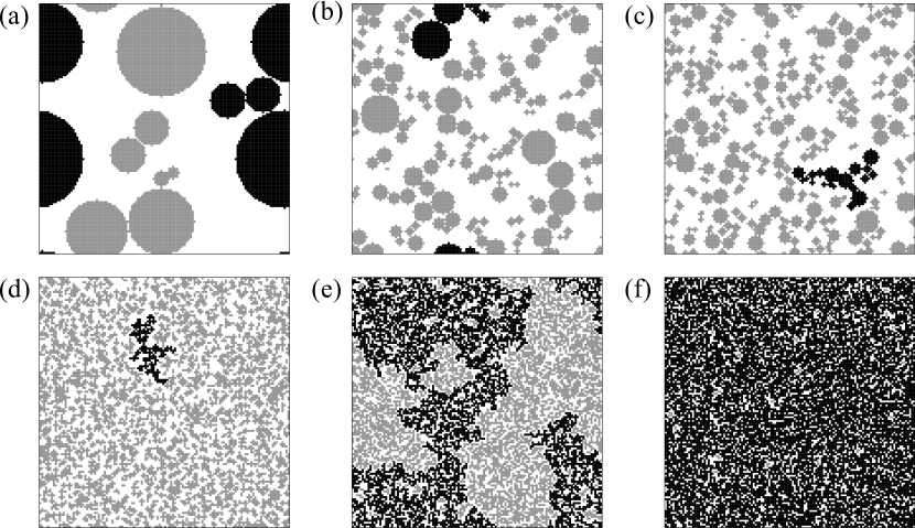
Figure 7: Samples of final configurations obtained for the CGP-D model on $2D$ square lattices of side length $L\!=\!128$ using disk-shaped cluster growth. The snapshots relate to different values of the initial density of active seed sites: $p\!=\!0.001$, $0.01$, $0.02$, $0.2$, $0.495$, $0.7$, for subfigures (a–f), respectively. In the limit of large system sizes and above the critical point $p_{c}\approx 0.497$, the largest cluster in the final configuration spans the lattice along at least one direction. In each subfigure, the largest cluster is colored black and all finite clusters are colored grey.

Appendix B Results for disk-shaped cluster growth

Assuming a circular shape of the growing clusters (see Fig. 7), and upon analysis of the order parameter (again for square systems with side-length up to $L=1024$), we yield the following results for the critical properties of the $2D$ “Touch and stop” cluster growth model:

Binder ratio:

Considering the Binder ratio, the best data collapse (obtained in the range $\epsilon\in[-2,2]$) yields $p_{c}=0.4978(3)$, and $\nu=1.32(4)$ with a quality $S=0.984$.

Order parameter:

Considering the relative size of the largest cluster found in the final configuration, the best data collapse (obtained in the range $\epsilon\in[-1,1]$) yields $p_{c}=0.4974(1)$, $\nu=1.29(3)$, and $\beta=0.145(4)$ with a quality $S=0.29$.

Order parameter fluctuations:

A best data collapse for the order parameter fluctuations (attained in the range $\epsilon\in[-1.5,1.5]$) results in the estimates $p_{c}=0.4978(5)$, $\nu=1.33(2)$, and $\gamma=2.38(3)$ with a quality $S=0.89$.

Cluster size distribution:

At the critical point, the algebraic decay of the probability mass function $n_{s}$ for clusters of size $s$ is governed by the exponent $\tau=2.050(6)$. This estimate was obtained for the data recorded at $L=1024$, using a least-squares fit to the interval $s\in[500,7000]$ (as before, the errorbar was estimated via bootstrap resampling).

The observation that the critical points for rhombic and disk-shaped cluster growth differ only slightly can be understood from the time evolution of the individual clusters. At short times (i.e. $t\leq 2$) both “growth styles” feature identical clusters. Only at times $t>2$, the disk-shaped growth style leads to more convex clusters that assume a circular shape in the limit $t\to\infty$. Close to the critical points of both growth styles, the cluster growth procedure stops after maximally $4$ time steps (i.e. at $t=4$). Thereby, the majority of initial seeds grow for less than 4 time steps and become inactive in a state where one cannot tell apart clusters that were grown using a rhombic or disk-shaped growth rule. Note that this is due to the discreteness of the underlying lattice.

References

- Stauffer (1979) D. Stauffer, Phys. Rep. 54, 1 (1979).
- Stauffer and Aharony (1994) D. Stauffer and A. Aharony, Introduction to Percolation Theory (Taylor and Francis, London, 1994).
- Pfeiffer and Rieger (2002) F. O. Pfeiffer and H. Rieger, J. Phys.: Condens. Matter 14, 2361 (2002).
- Pfeiffer and Rieger (2003) F. O. Pfeiffer and H. Rieger, Phys. Rev. E 67, 056113 (2003).
- Cieplak et al. (1994) M. Cieplak, A. Maritan, and J. R. Banavar, Phys. Rev. Lett. 72, 2320 (1994).
- Melchert and Hartmann (2007) O. Melchert and A. K. Hartmann, Phys. Rev. B 76, 174411 (2007).
- Schwarz et al. (2009) K. Schwarz, A. Karrenbauer, G. Schehr, and H. Rieger, J. Stat. Mech. 2009, P08022 (2009).
- Mertens and Moore (2012) S. Mertens and C. Moore (2012), preprint: arXiv:1209.4936.
- Tsakiris et al. (2010a) N. Tsakiris, M. Maragakis, K. Kosmidis, and P. Argyrakis (2010a), preprint: arXiv:1004.1526v2; A summary of this article is available at papercore.org, see http://www.papercore.org/Tsakiris2010a.
- Tsakiris et al. (2010b) N. Tsakiris, M. Maragakis, K. Kosmidis, and P. Argyrakis (2010b), preprint: arXiv:1004.5028; A summary of this article is available at papercore.org, see http://www.papercore.org/Tsakiris2010.
- Houdayer and Hartmann (2004) J. Houdayer and A. K. Hartmann, Phys. Rev. B 70, 014418 (2004).
- Melchert (2009) O. Melchert, Preprint: arXiv:0910.5403v1 (2009).
- Binder (1981) K. Binder, Z. Phys. B 43, 119 (1981).
- Sur et al. (1976) A. Sur, J. L. Lebowitz, J. Marro, M. H. Kalos, and S. Kirkpatrick, J. Stat. Phys. 15, 345 (1976).
- Newman and Ziff (2000) M. Newman and R. Ziff, Phys. Rev. Lett. 85, 4104 (2000), A summary of this article is available at papercore.org, see http://www.papercore.org/Newman2000.
- Wikipedia (2012) Wikipedia, Percolation threshold — Wikipedia, the free encyclopedia (2012), online; accessed 27-August-2012, URL http://en.wikipedia.org/wiki/Percolation_threshold.
- Argyrakis (2012) P. Argyrakis (2012), private communication.