Tearing the veil: interaction of the Orion Nebula with its neutral environment

Abstract

We present H i $21\;\hbox{\rm cm}$ observations of the Orion Nebula, obtained with the Karl G. Jansky Very Large Array, at an angular resolution of ${7^{\prime\prime}\hskip-4.60007pt.\hskip 1.19995pt2}\times{5^{\prime\prime}\hskip-4.60007pt.\hskip 1.19995pt7}$ and a velocity resolution of $0.77\;\hbox{\rm km}\;\hbox{\rm s}^{-1}$. Our data reveal H i absorption towards the radio continuum of the H ii region, and H i emission arising from the Orion Bar photon-dominated region (PDR) and from the Orion-KL outflow. In the Orion Bar PDR, the H i signal peaks in the same layer as the $\hbox{\rm H}_{2}$ near-infrared vibrational line emission, in agreement with models of the photodissociation of $\hbox{\rm H}_{2}$. The gas temperature in this region is approximately $540\;\hbox{\rm K}$, and the H i abundance in the interclump gas in the PDR is 5–10% of the available hydrogen nuclei. Most of the gas in this region therefore remains molecular. Mechanical feedback on the Veil manifests itself through the interaction of ionized flow systems in the Orion Nebula, in particular the Herbig-Haro object ${\rm HH}\,{\rm 202}$, with the Veil. These interactions give rise to prominent blueward velocity shifts of the gas in the Veil. The unambiguous evidence for interaction of this flow system with the Veil shows that the distance between the Veil and the Trapezium stars needs to be revised downwards to about $0.4\;\hbox{\rm pc}$. The depth of the ionized cavity is about $0.7\;\hbox{\rm pc}$, which is much smaller than the depth and the lateral extent of the Veil. Our results reaffirm the blister model for the M42 H ii region, while also revealing its relation to the neutral environment on a larger scale.

1. Introduction

The Orion Nebula (M42, ${\rm NGC}\,{\rm 1976}$, Orion A) is the nearest region of recent massive star formation, containing the densest nearby cluster of OB stars. Since the optically visible nebula M42 is located in front of the parent molecular cloud OMC-1, it is accessible for detailed studies in every region of the electromagnetic spectrum. As a result, the Orion Nebula has become a cornerstone for our understanding of massive star formation, as well as its feedback effects on the star forming environment, which is the subject of the present paper.

The Orion nebula and OMC-1 are located near the center of a prominent north-south ridge of dense molecular gas, shaped approximately like an integral sign (Bally et al., 1987; Castets et al., 1990; Heyer et al., 1992; Johnstone & Bally, 1999; Plume et al., 2000), and containing the OMC-1 through OMC-4 molecular clumps. OMC-1 is the most most prominent of these, with a mass of approximately $2200\;\hbox{\rm M}_{\odot}$ (Bally et al., 1987). The integral-shaped ridge is the northern part of the larger Orion A giant molecular cloud (GMC), which has a mass of about $10^{5}\;\hbox{\rm M}_{\odot}$ (Maddalena et al., 1986) and is one of a system of two GMCs (the Orion A and Orion B GMCs, named after the radio sources they contain) that extends roughly north-south through the belt and sword regions of the Orion constellation (Kutner et al., 1977; Maddalena et al., 1986; Sakamoto et al., 1994; Wilson et al., 2005). These clouds are associated with even larger diffuse H i clouds (Chromey et al., 1989; Green, 1991). An excellent recent review of star formation and molecular clouds in the greater Orion region has been presented by Bally (2008).

The Orion A molecular cloud hosts several generations of OB star formation (Blaauw, 1964), the youngest of which is the Orion Nebula Cluster (ONC), ionizing the M42 H ii region (see Muench et al., 2008, for a detailed recent review). This cluster has a central density of about $2\times 10^{4}\,$stars$\;\hbox{\rm pc}^{-3}$ and a total stellar mass of about $1800\;\hbox{\rm M}_{\odot}$ in about 3500 stars (Hillenbrand & Hartmann, 1998), out to a radius of $\sim 2.5\;\hbox{\rm pc}$. The total mass of the ONC is therefore comparable to the molecular gas mass of OMC-1, which is $2200\;\hbox{\rm M}_{\odot}$, within a similar radius (Bally et al., 1987). Locally, the star formation efficiency (here quantified as $M_{\rm stars}/(M_{\rm stars}+M_{\rm gas})$) is therefore quite high at approximately 50%. On the scale of the integral-shaped ridge (linear size about $9\;\hbox{\rm pc}$), which has a gas mass of $\sim 5000\;\hbox{\rm M}_{\odot}$ (Bally et al., 1987), this efficiency is somewhat lower, approximately 25%. The ionizing luminosity of the ONC is dominated by $\theta^{1}$ C Ori. This star is the most luminous component of the asterism formed by the Trapezium stars ($\theta^{1}$ A–D Ori). $\theta^{1}$ C Ori is an oblique magnetic rotator with an effective temperature $T_{\rm eff}\approx 39000\pm 1000\;\hbox{\rm K}$ and $\log g=4.1$ (Simón-Díaz et al., 2006), implying a spectral type O6Vp. Observations by Weigelt et al. (1999) revealed that $\theta^{1}$ C Ori is a close binary, dominated in mass and luminosity by the star $\theta^{1}$ C₁ Ori, for which a spectral type O5.5 was derived by Kraus et al. (2007). The ionizing photon flux corresponding to spectral types O6 to O5.5 is $Q_{0}=1.0-1.3\cdot 10^{49}\;\hbox{\rm s}^{-1}$ (Martins et al., 2005).

Most visual studies of the Orion Nebula have concentrated on the $\sim 5^{\prime}$ diameter optically bright region centered on the Trapezium stars, commonly referred to as the Huygens region, after its first description by Huygens (1659). However, lower surface brightness nebular emission extends significantly towards the southwest. Including this fainter region the nebula subtends an approximately circular region on the sky, with a diameter of about half a degree (e.g., Fig. 1 in Muench et al., 2008). This region is now referred to as the Extended Orion Nebula (EON, Güdel et al., 2008) and contains the Huygens region at its north-east boundary. The Huygens region itself is bounded at the northeast side by the Northeast Dark Lane (O’Dell & Harris, 2010), which separates M42 from the fainter H ii region M43 towards the northeast. Another prominent dark feature, already seen by Huygens (1659) is the Dark Bay, which is a tongue of obscuration, covering part of M42 east of the Trapezium stars.

The Orion Nebula is a blister-type H ii region, with the ionized gas streaming away from the high pressure interface with OMC-1 (Zuckerman, 1973; Balick et al., 1974). Velocities with respect to the Local Standard of Rest (LSR) in the ionized gas are $v_{\rm LSR}=7.4\pm 1.5\;\hbox{\rm km}\;\hbox{\rm s}^{-1}$ for the low ionization lines ([O i], [S ii]) arising at the ionization front (IF), but lower (i.e., more blueshifted) velocities $v_{\rm LSR}=-0.2\pm 1.3\;\hbox{\rm km}\;\hbox{\rm s}^{-1}$ are found for higher excitation species ([O ii], [O iii], [N ii]) and for the bulk ionized gas traced by hydrogen recombination lines (Kaler, 1967; O’Dell & Wen, 1992; Doi et al., 2004; Henney et al., 2007; García-Díaz & Henney, 2007; García-Díaz et al., 2008). The background molecular gas is at $v_{\rm LSR}\approx 10\;\hbox{\rm km}\;\hbox{\rm s}^{-1}$(Loren, 1979). The ionization front (IF) separating M42 and OMC-1 is located behind the Trapezium stars, at a distance of approximately $0.3\;\hbox{\rm pc}$ behind $\theta^{1}$ C Ori (Wen & O’Dell, 1995; O’Dell, 2001; O’Dell et al., 2008). A three-dimensional model of the ionized region has been derived by Wen & O’Dell (1995), who showed that the IF, which is approximately face-on in the region behind the Trapezium stars, curves to an orientation that is almost edge-on approximately $100^{\prime\prime}$ south-east of the Trapezium stars. In this region the IF is observed as a prominent, almost linear optical feature commonly referred to as the Bright Bar. On the molecular side of the IF, a photon-dominated region (PDR) has formed, which is close to edge-on south-east of the Bright Bar. It has been studied in the strong neutral gas cooling lines, in particular [C ii] $158\;\mu\hbox{\rm m}$ (Stacey et al., 1993) and [O i] $63\;\mu\hbox{\rm m}$ (Herrmann et al., 1997) as well as numerous other species. Due to its aspect and proximity, the edge-on Orion Bar PDR has become the most iconic region of its type.

The OMC-1 molecular cloud behind M42 harbors an obscured region of young massive star formation, exhibiting luminous infrared emission with a bolometric luminosity of about $8\cdot 10^{4}\;\hbox{\rm L}_{\odot}$ (Gezari et al., 1998), known as the Kleinmann-Low region (Orion-KL, Kleinmann & Low, 1967), and located about $1^{\prime}$ northwest of the Trapezium stars. This region contains a complex system of outflows and masers, various young stellar objects, and the eponymous Orion Hot Core, a compact region of molecular gas and dust with high temperature (several $100\;\hbox{\rm K}$) and density ($\sim 10^{6}\;\hbox{\rm cm}^{-3}$) driving a complex chemistry. The high velocity outflow originating in this region gives rise to the famous “fingers”, first discussed by Allen & Burton (1993). All of these features are the subject of a vast literature, to which we will return in Sect. 6.3. Extensive background can be found in the review by Genzel & Stutzki (1989), which contains an overview and synthesis of earlier results, and the review by O’Dell et al. (2008), which discusses more recent results on this complex region.

A second active star forming region is located about ${1^{\hskip 0.35002pt\prime}\hskip-3.50006pt.\hskip 0.50003pt5}$ south of Orion-KL. This region, referred to as Orion-S, has an infrared luminosity of about 10% of that of Orion-KL (Mezger et al., 1990). Like Orion-KL, Orion-S is a rich source of molecular line emission, containing several hot cores (Zapata et al., 2007) and multiple bipolar outflows and maser systems. However, unlike Orion-KL, Orion-S is an isolated molecular core located within the cavity containing the ONC (O’Dell et al., 2009). As a result several of the outflows originating from Orion-S produce optically detectable features, many of which are catalogued as Herbig-Haro (HH) objects (O’Dell et al., 1997; Bally et al., 2000; Henney et al., 2007; O’Dell & Henney, 2008).

In front of the ionized nebula, several layers of predominantly neutral atomic gas are found. These were first detected in $21\;\hbox{\rm cm}$ H i absorption towards the nebular radio continuum (Muller, 1959; Clark et al., 1962; Clark, 1965; Radhakrishnan et al., 1972; Lockhart & Goss, 1978), and are collectively referred to as the Veil (O’Dell, 2001). The term Veil is appropriate since this feature is largely transparent, and only becomes opaque (at visual wavelengths) in the Dark Bay and Northeast Dark Lane regions, where its column density is highest (O’Dell & Yusef-Zadeh, 2000). The first full H i aperture synthesis observations of the Orion Nebula were carried out by Lockhart & Goss (1978) at an angular resolution of $2^{\prime}$, using the Owens Valley Interferometer. These authors first showed the presence of 3 velocity components in the Veil. This velocity structure was confirmed in higher resolution ($16^{\prime\prime}$) aperture synthesis using the VLA in C-configuration (Van der Werf & Goss, 1989, hereafter vdWG89), who found LSR velocities of approximately 6, 4, and $-2\;\hbox{\rm km}\;\hbox{\rm s}^{-1}$ for the absorbing components A, B and C (adopting the notation of vdWG89, which we follow in the present paper). These observations confirmed the physical association of the Veil with the Orion Nebula, first suggested by Lockhart & Goss (1978), based on the increasing H i column density towards the Dark Bay and Northeast Dark Lane in the velocity components A and B. Absorption by components A and B is also detected towards the smaller H ii region M43 towards the northeast, confirming that the Veil represents an extended layer covering the M42/M43 system. The total H i opacity distribution of components A and B correlates well with the optical extinction towards the Huygens region (O’Dell et al., 1992; O’Dell & Yusef-Zadeh, 2000). Physical conditions in the Veil have been studied further by optical (O’Dell et al., 1993) and ultraviolet (UV) absorption lines (Abel et al., 2004, 2006; Lykins et al., 2010). Modeling of these results has resulted in a location for the Veil of a significant, but not accurately determined, distance of $1-3\;\hbox{\rm pc}$ in front of the Trapezium stars (Abel et al., 2004).

Several additional H i absorption components have been detected towards the Huygens region. These cover only small parts of M42 and are not detected towards M43. Velocity component C at $v_{\rm LSR}\approx-2\;\hbox{\rm km}\;\hbox{\rm s}^{-1}$ was already detected by Lockhart & Goss (1978). The H i observations described by vdWG89 unexpectedly revealed a remarkable set of small-scale ($0.02-0.06\;\hbox{\rm pc}$) H i absorption components (Van der Werf & Goss, 1990, hereafter vdWG90). Most of these features (D–G in the notation of vdWG90) are blueshifted with respect to both the molecular and the ionized gas, and have central LSR velocities from $-7$ to $-17\;\hbox{\rm km}\;\hbox{\rm s}^{-1}$. Two of the features exhibited several velocity components. In addition, one feature (H) was detected by vdWG90 in absorption at the velocity of the background molecular cloud OMC-1. The features are most likely associated with M42 (vdWG90), but their precise nature remained somewhat unclear.

In the present paper, we return to the Orion Nebula to investigate the radiative and mechanical feedback of the ONC, the Orion Nebula and the various outflow systems, on the neutral environment of the nebula. We use new high resolution H i radio observations to probe H i emission from behind the Huygens region and from the Orion Bar PDR, as well as H i absorption from the Veil and the small-scale absorption components. We thus obtain a comprehensive picture of the radiative and mechanical feedback effects of massive star formation in this region on the neutral gas environment. We describe the observations and data reduction in Sect. 2. The radio continuum, H i emission, and H i absorption results are presented in Sects. 3–5. These results are discussed in detail in Sects. 6 and 7. Finally, our conclusions are summarized in Sect. 9. Throughout this paper, we adopt a distance to the Trapezium stars of $436\pm 20\;\hbox{\rm pc}$ as given by O’Dell & Henney (2008), which is based on a weighted combination of several parallax measurements (Genzel et al., 1981; Kraus et al., 2007; Menten et al., 2007; Hirota et al., 2007). At this distance, $1^{\prime\prime}=0.0023\;\hbox{\rm pc}$ or $436\;\hbox{\rm AU}$. Where we use distance-dependent quantities from earlier publications, we have tacitly converted these to the distance adopted here.

2. Observations and reduction

2.1. Observations

We used the NRAO Karl G. Jansky Very Large Array (VLA), to obtain H i data of the Orion Nebula in two periods in 2006 and 2007 (programs AG738 and AV297). The C and then the B array of the VLA were used to extend the angular resolution, sensitivity and velocity coverage of the old C array data of vdWG89 and vdWG90, obtained in 1984. The VLA correlator was used. The total bandwidth was $781.25\;\hbox{\rm kHz}$ with 256 channels and two circular polarizations, centered at $v_{\rm LSR}=2.0\;\hbox{\rm km}\;\hbox{\rm s}^{-1}$. The channel separation was $3.052\;\hbox{\rm kHz}$ ($0.64\;\hbox{\rm km}\;\hbox{\rm s}^{-1}$ at the H i line) and the velocity resolution was $0.77\;\hbox{\rm km}\;\hbox{\rm s}^{-1}$.

The C array data was obtained in a series of three 5 hour observations on 2006 September 29, November 9 and November 19. Twenty of the VLA antennas were used, with no use of the 7 antennas that had been converted to the EVLA at that time. The phase calibration was based on frequent observations (once per half hour) of the quasar ${\rm OG}\,{\rm 050}$ (J0532+0732) with a flux density of $1.8\;\hbox{\rm Jy}$. The flux density scale was set by observations of ${\rm 3C}\,{\rm 48}$ ($15.7\;\hbox{\rm Jy}$).

The B array data were obtained during late 2007 in a three times 5 hour observation on November 15, November 24 and December 3. The flux density scale was set using observations of ${\rm 3C}\,{\rm 138}$ (total flux density $8.3\;\hbox{\rm Jy}$). The observations of ${\rm 3C}\,{\rm 138}$ were carried out every 30 minutes for a period of 4 minutes.

For both the C array and the B array data, bandpass responses of each antenna were determined by observing the strong sources ${\rm 3C}\,{\rm 48}$ and ${\rm 3C}\,{\rm 84}$; these observations were shifted by plus and minus $0.7\;\hbox{\rm MHz}$ ($148\;\hbox{\rm km}\;\hbox{\rm s}^{-1}$) to avoid the H i emission near $v_{\rm LSR}=0\;\hbox{\rm km}\;\hbox{\rm s}^{-1}$ and absorption lines of Galactic H i in the spectra of the calibration sources.

2.2. Reduction and generation of data cubes

During the 2007 observations, we used EVLA antennas for the first time. At this time there were 12 EVLA antennas and 13 VLA antennas. During a test observation of ${\rm 3C}\,{\rm 48}$ obtained on 2007 October 4, an aliasing problem with the old VLA correlator and the use of EVLA baselines was discovered by a number of NRAO staff (including M. Goss). This problem was caused by the hardware used to convert the digital signals from the EVLA antennas into analogue signals to be fed in the VLA correlator, which caused power to be aliased into the bottom $0.5\;\hbox{\rm MHz}$ of the baseband. Only EVLA to EVLA antenna correlations were affected. A number of partial solutions were found. For the Orion A H i observations, the solution adopted was to use observations of the strong source ${\rm 3C}\,{\rm 138}$ every 30 minutes and to apply a time variable baseline based calibration (as opposed to an antenna based calibration) to correct for the closure errors due to the mismatched and time variable bandpasses resulting from the aliasing. This scheme was tested in detail using the correlator configuration that we used for the Orion A H i observations. We found that tracking the errors over this time interval worked well and the visibility functions of the calibrator sources for EVLA to EVLA baselines had a similar behavior as those of the VLA to VLA baselines. Before the phase closure corrections were made, the amplitude fluctuations were at the level of 15% ($1\sigma$) of the continuum flux density of ${\rm 3C}\,{\rm 138}$; after correction the fluctuations were reduced to values well below $2\%$. With the advent of the WIDAR correlator in early 2010, these aliasing problems have disappeared.

The data from the C and B arrays were then combined and the line images were made after subtracting the continuum in the uv plane (using the AIPS task UVLSF); 102 of the 255 channels were line free and formed the continuum. The final images were made using the AIPS task IMAGR with Robust=0 weighting. The resulting datacube has a synthesized beam of ${7^{\prime\prime}\hskip-4.60007pt.\hskip 1.19995pt2}\times{5^{\prime\prime}\hskip-4.60007pt.\hskip 1.19995pt7}$ at a position angle of $29.7^{\circ}\hskip-2.84544pt$ and an r.m.s. noise per channel of $40\;\hbox{\rm K}$. The conversion factor between brightness temperature and flux density is $14.9\;\hbox{\rm K}\,({\rm mJy}\;\hbox{\rm beam}^{-1})^{-1}$. A $1420.4\;\hbox{\rm MHz}$ image was produced using a multiscale CLEAN algorithm, in order to optimally preserve the large range of spatial scales present in this image. The measured r.m.s. noise in the continuum image is $3.1\;\hbox{\rm mJy}\;\hbox{\rm beam}^{-1}$.

In the spectral line data cube, we discarded channels with elevated noise at the edges of the band. Our final data cube covers the range $-62.00\;\hbox{\rm km}\;\hbox{\rm s}^{-1}<v_{\rm LSR}<68.56\;\hbox{\rm km}\;\hbox{\rm s}^{-1}$.

2.3. Further processing

Inspection of the H i data cube revealed a large and complex set of features at various velocities, and with various angular sizes. Remarkably, H i is detected in both emission and absorption.

Interferometric imaging of extended low-level emission features in the presence of a strong continuum requires careful processing, because of non-linearities introduced by deconvolution algorithms such as CLEAN (see e.g., Van Gorkom & Ekers, 1989), which may give rise to spurious features after continuum subtraction. The best way to avoid these problems consists of first subtracting the continuum and applying the deconvolution to the continuum-free line images. As described above, this is the procedure that was used. After continuum subtraction the H i absorption produces a strong negative signal carrying the imprint of the subtracted continuum at LSR velocities between $-20$ and $10\;\hbox{\rm km}\;\hbox{\rm s}^{-1}$; at other velocities any remaining signal results from H i emission. As a result, H i emission can only reliably be studied at velocities outside the range from $-20$ to $10\;\hbox{\rm km}\;\hbox{\rm s}^{-1}$. In order to increase the S/N ratio of the H i emission data, we convolved the channel maps to a ${7^{\prime\prime}\hskip-4.60007pt.\hskip 1.19995pt5}$ circular beam, and smoothed the data cube spectrally by a factor 2, i.e., to a velocity resolution and channel separation of $1.29\;\hbox{\rm km}\;\hbox{\rm s}^{-1}$. The r.m.s. noise in brightness temperature $T_{\rm b}$ in these images is $20\;\hbox{\rm K}$. Since the shortest baselines in our observations were about $73\;\hbox{\rm m}$, our data are insensitive to structures with scales of about $7^{\prime}$ or more.

In order to study the H i absorption, the full spatial and spectral resolution H i line data cube was used, with the corresponding $1420.4\;\hbox{\rm MHz}$ continuum image, to derive a data cube of H i optical depth $\tau$, following the approach of vdWG89. Optical depths were derived by solving the equation of transfer

$$T_{\rm b}(v)=[1-e^{-\tau(v)}][T_{\rm s}-T_{\rm c}-T_{\rm back}(v)],$$ (1)

where $T_{\rm b}(v)$ is the observed H i brightness temperature at LSR velocity $v$, after subtraction of the continuum (which has brightness temperature $T_{\rm c}$). $T_{\rm s}$ is the spin temperature of the absorbing H i, and $T_{\rm back}(v)$ is the brightness temperature (at LSR velocity $v$) of Galactic H i originating behind the absorbing H i. The peak brightness temperature of Galactic H i in the region of the Orion Nebula is about $60\;\hbox{\rm K}$ (Green, 1991). It is not possible to determine what fraction of this signal originates behind the absorbing H i, and the situation is complicated further by the fact that this fraction may be a function of $v$. Therefore the observed Galactic H i brightness temperature only provides an upper limit for $T_{\rm back}(v)$. For $T_{\rm s}$ a harmonic mean value can be determined at positions where H i $21\;\hbox{\rm cm}$ absorption can be combined with measurements of $\hbox{{\rm Ly}}\alpha$ absorption. Such measurements are available at the positions of $\theta^{1}$ C Ori (Shuping & Snow, 1997) and $\theta^{1}$ B Ori (Abel et al., 2006), giving $T_{\rm s}\approx 90\;\hbox{\rm K}$ ($80{-}110\;\hbox{\rm K}$) in component A and $T_{\rm s}\approx 135\;\hbox{\rm K}$ ($100{-}160\;\hbox{\rm K}$) in component B. Given the uncertainties in $T_{\rm s}$ and $T_{\rm back}(v)$ we solve Eq. $\left(\ref{eq.Transfer}\right)$ with the approximation $T_{\rm c}\gg\left|T_{\rm s}-T_{\rm back}(v)\right|$, by only calculating opacities at positions where $T_{\rm c}>450\;\hbox{\rm K}$ (corresponding to a surface brightness level of $30\;\hbox{\rm mJy}\;\hbox{\rm beam}^{-1}$), which is almost $10\sigma$ in the continuum image. While H i absorption lines can be detected towards considerably fainter continuum levels, quantitatively reliable opacities can only be derived where $T_{\rm c}\gg\left|T_{\rm s}-T_{\rm back}(v)\right|$. With this approach the precise value of $T_{\rm s}$ for determining the opacities (as well as the implicit assumption of Eq. $\left(\ref{eq.Transfer}\right)$ that $T_{\rm s}$ is the same at every position and for all absorbing velocity components) becomes irrelevant. At positions with $T_{\rm c}\leq 450\;\hbox{\rm K}$, this procedure will give rise to systematic errors in the derived opacities; at these positions opacities are therefore not calculated.

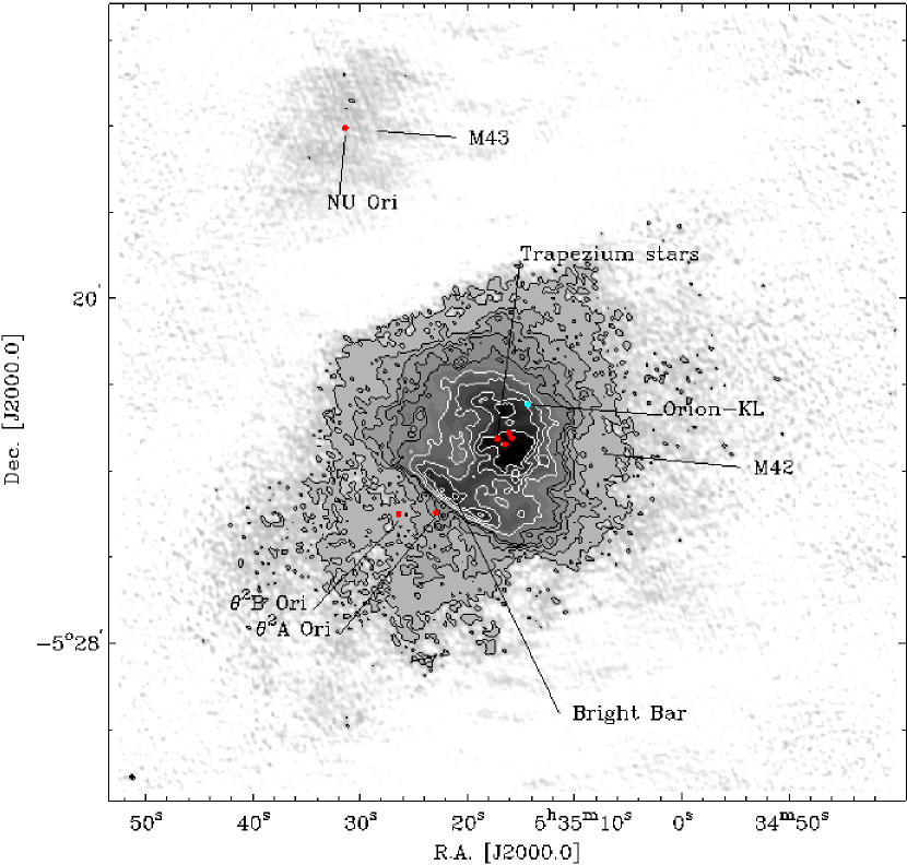
Figure 1.— Continuum emission of the Orion Nebula at $1420.4\;\hbox{\rm MHz}$, constructed using a multi-scale deconvolution (see Sect. 2.2). Contours indicate surface brightness levels of 20, 40, 60, 80 and $100\;\hbox{\rm mJy}\;\hbox{\rm beam}^{-1}$ (black contours) and 150, 200, 250, 300 and $350\;\hbox{\rm mJy}\;\hbox{\rm beam}^{-1}$ (white contours). The small ellipse in the lower lefthand corner indicates the FWHM size and the orientation of the synthesized beam (${7^{\prime\prime}\hskip-4.60007pt.\hskip 1.19995pt2}\times{5^{\prime\prime}\hskip-4.60007pt.\hskip 1.19995pt7}$ at a position angle of $29.7^{\circ}\hskip-2.84544pt$). The image has been corrected for primary beam attenuation. The principal massive young stars are indicated by red dots. A cyan dot indicates the position of the Orion-KL region.

3. Continuum emission

The $1420.4\;\hbox{\rm MHz}$ continuum image is shown in Fig. 1. This image shows both the main H ii region M42 and the fainter H ii region M43 in the northeast. The image of M42 is dominated by the Huygens region and the Bright Bar in the southeast. Fainter emission from the EON is seen to extend in all directions from the southeast counterclockwise to the West, but not in the other directions. Indications for the presence of low surface brightness radio emission from the EON were first found by Mills & Shaver (1968) and Goss & Shaver (1970). Emission from the full EON is detected in the $4.75\;\hbox{\rm GHz}$ single-dish image of Wilson et al. (1997) and in the $330\;\hbox{\rm MHz}$ VLA image of Subrahmanyan et al. (2001); the $1.5\;\hbox{\rm GHz}$ VLA image by Yusef-Zadeh (1990) and Subrahmanyan et al. (2001) also shows the extended emission from the EON.

The total flux density of M42 in our image is $335\pm 15\;\hbox{\rm Jy}$. This value is somewhat lower than the total flux density of $374\;\hbox{\rm Jy}$ found by vdWG89 (which is consistent with the best single-dish value, see Table 2 in vdWG89). For M43, we find a total flux density of $14\pm 2\;\hbox{\rm Jy}$, in excellent agreement with vdWG89.

The peak continuum flux density of M42 is $376\;\hbox{\rm mJy}\;\hbox{\rm beam}^{-1}$, which corresponds to a peak continuum brightness temperature $T_{\rm c}=5600\;\hbox{\rm K}$. The electron temperature in this region is $T_{\rm e}=8400\pm 400\;\hbox{\rm K}$, as determined by Wilson et al. (1997) from measurements of the H64$\alpha$ recombination line. Since $T_{\rm c}=T_{\rm e}(1-e^{-\tau_{\rm ff}})$, the peak free-free optical depth is $\tau_{\rm ff}=1.1$, i.e., the H ii region is significantly optically thick at $1420.4\;\hbox{\rm MHz}$, and will be opaque at lower frequencies, in agreement with the spectral index distribution between 330 and $1500\;\hbox{\rm MHz}$ determined by Subrahmanyan et al. (2001). A free-free opacity $\tau_{\rm ff}\approx 1$ is also found at the brightest peaks of the Bright Bar.

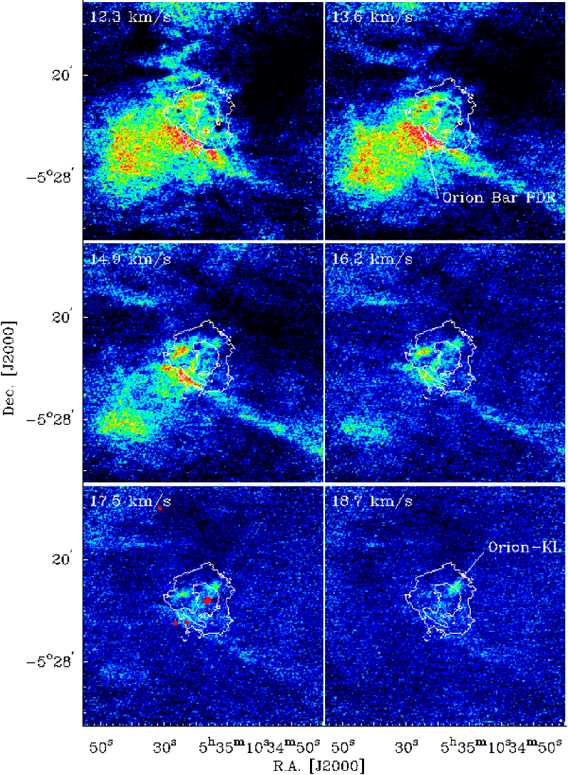
Figure 2.— Images of H i emission at the LSR velocities indicated in the upper left-hand corner of each frame. The images cover a velocity interval of $1.28\;\hbox{\rm km}\;\hbox{\rm s}^{-1}$ each. Colors ranging from dark blue to red indicate a brightness temperature range from 0 to $250\;\hbox{\rm K}$. White contours indicate the $21\;\hbox{\rm cm}$ continuum at levels of 50 and $200\;\hbox{\rm mJy}\;\hbox{\rm beam}^{-1}$. These images have been corrected for primary beam attenuation. The ${7^{\prime\prime}\hskip-4.60007pt.\hskip 1.19995pt5}$ circular beam of these images is indicated in the lower righthand corner. The red dots in the lower left panel indicate the principal young massive stars (see Fig. 1 for legend).

4. H i emission features

4.1. H i emission images

As noted in Sect. 2.3, H i emission can be studied at velocities avoiding strong absorption, i.e., outside the velocity interval from $-20$ to $10\;\hbox{\rm km}\;\hbox{\rm s}^{-1}$. Since the prominent molecular cloud associated with the Orion Nebula is at $v_{\rm LSR}\sim 10\;\hbox{\rm km}\;\hbox{\rm s}^{-1}$, H i emission from the neutral environment of the H ii region can be probed only in its red line wing. Inspection of the H i emission data cube revealed H i emission at LSR velocities from 10 to $19\;\hbox{\rm km}\;\hbox{\rm s}^{-1}$, and six images covering this velocity range are presented in Fig. 2.

Inspection of Fig. 2 reveals that the strongest H i emission is found in the region directly southeast of the Bright Bar. H i brightness temperatures in this region are approximately $250\;\hbox{\rm K}$ (coded red in Fig. 2), with peaks reaching $300\;\hbox{\rm K}$, indicating that the gas is quite warm. While the brightest H i emission is found closest to the Bar, the emission extends towards the southeast over a distance of about $6^{\prime}$ ($0.8\;\hbox{\rm pc}$), at brightness temperature levels of about $120\;\hbox{\rm K}$. Other features worthy of note are an elongated H i feature extending from the Bar region towards the southwest at velocities of $13-16\;\hbox{\rm km}\;\hbox{\rm s}^{-1}$, and compact H i emission features with higher velocities ($v_{\rm LSR}$ up to $19\;\hbox{\rm km}\;\hbox{\rm s}^{-1}$). H i emission features northeast of M42 trace the direct environment of M43.

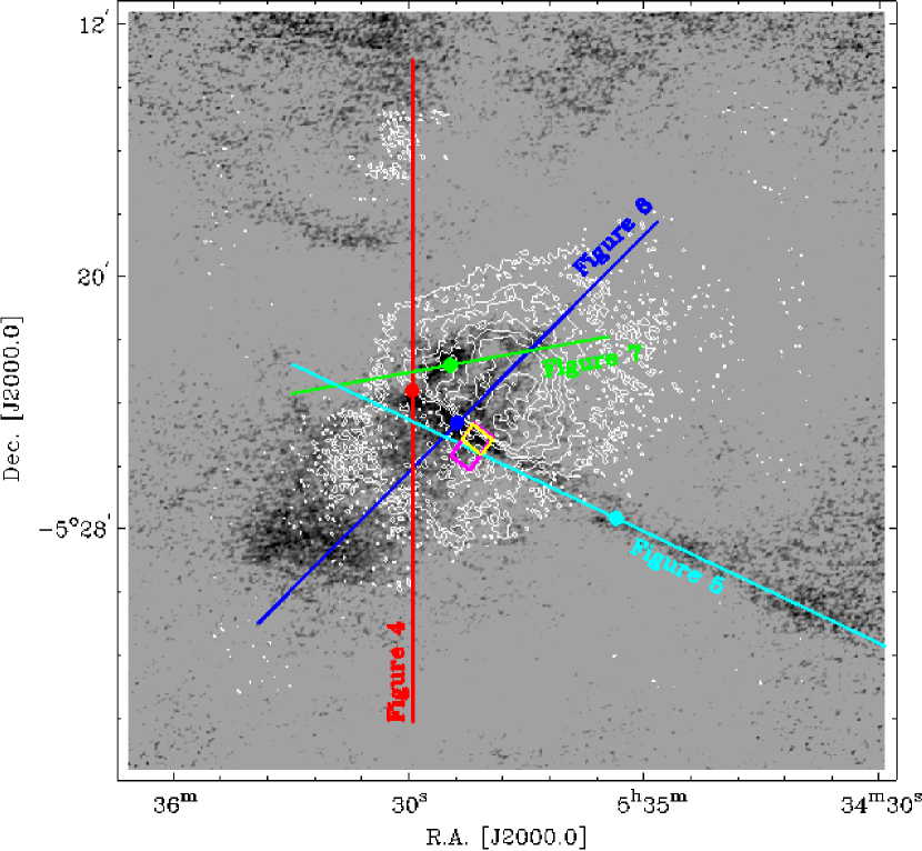
Figure 3.— Location of the position-velocity (PV) diagrams of H i emission shown in Figs. 4–7, superposed on an H i emission image at $v_{\rm LSR}=14.9\;\hbox{\rm km}\;\hbox{\rm s}^{-1}$ (greyscale). The precise lengths, orientations and positions of these PV diagrams are indicated by the colored bars. In each bar, a thick dot of the same color indicates the zero position of the spatial coordinate in the corresponding PV diagram. The relevant figure numbers are indicated. White contours indicate $1420.4\;\hbox{\rm MHz}$ continuum surface brightnesses of 15, 40, 70, 100, 150, 200 and $300\;\hbox{\rm mJy}\;\hbox{\rm beam}^{-1}$. The purple rectangle in the Bright Bar region indicates the region used for constructing the strip shown in Fig. 22. The yellow rectangle (which is contained in the purple one) shows the region over which the spectrum shown in Fig. 21 was averaged.

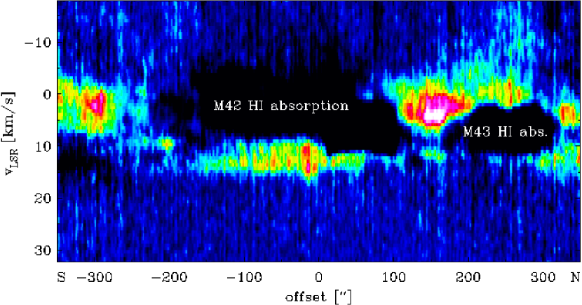
Figure 4.— Position-velocity diagram of H i emission along the red north-south bar shown in Fig. 3. The spatial axis has its zero position at $\hbox{\rm RA}=5^{\rm h}\,35^{\rm m}\,29^{\rm s}\hskip-3.9pt.\hskip 0.80002pt5$, $\hbox{\rm Dec}=-5^{\circ}\,23^{\prime}\,37^{\prime\prime}$ and a position angle of $0^{\circ}\hskip-2.84544pt$. Spatial offsets are positive towards the north and negative towards the south. Features discussed in the text are indicated.

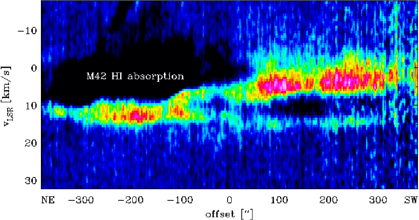
Figure 5.— Position-velocity diagram of H i emission along the light blue northeast-southwest bar shown in Fig. 3. The spatial axis has its zero position at $\hbox{\rm RA}=5^{\rm h}\,35^{\rm m}\,03^{\rm s}\hskip-3.9pt.\hskip 0.80002pt5$, $\hbox{\rm Dec}=-5^{\circ}\,27^{\prime}\,40^{\prime\prime}$ and a position angle of $64.66^{\circ}\hskip-2.84544pt$. Spatial offsets are negative towards the northest and positive towards the southwest. Features discussed in the text are indicated.

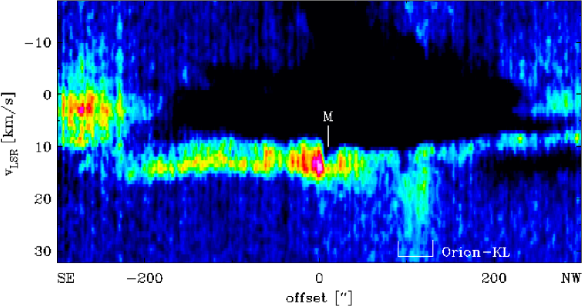
Figure 6.— Position-velocity diagram of H i emission along the dark blue northwest-southeast bar shown in Fig. 3. The spatial axis has its zero position at $\hbox{\rm RA}=5^{\rm h}\,35^{\rm m}\,23^{\rm s}\hskip-3.9pt.\hskip 0.80002pt8$, $\hbox{\rm Dec}=-5^{\circ}\,24^{\prime}\,38^{\prime\prime}$ and a position angle of $-45^{\circ}\hskip-2.84544pt$. Spatial offsets are negative towards the southeast and positive towards the northwest. Features discussed in the text are indicated.

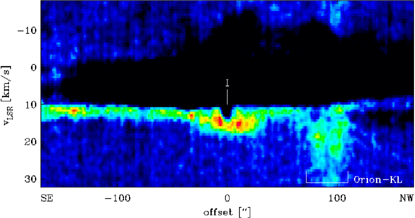
Figure 7.— Position-velocity diagram of H i emission along the green northwest-southeast bar shown in Fig. 3. The spatial axis has its zero position at $\hbox{\rm RA}=5^{\rm h}\,35^{\rm m}\,25^{\rm s}\hskip-3.9pt.\hskip 0.80002pt4$, $\hbox{\rm Dec}=-5^{\circ}\,22^{\prime}\,48^{\prime\prime}$ and a position angle of $-80^{\circ}\hskip-2.84544pt$. Spatial offsets are negative towards the southeast and positive towards the northwest. Features discussed in the text are indicated.

4.2. Position-velocity diagrams of H i emission

In order to study the velocity structure of the H i emission and its relation to the H i absorption (to be discussed below), we have constructed a number of position-velocity (PV) diagrams of the H i emission. The orientations of the spatial axes of these diagrams are shown in Fig. 3.

Figure 4 shows the velocity structure of the extended H i layers in the region of the Orion Nebula. A prominent H i layer can be seen in emission in the south (at an offset of approximately $-300^{\prime\prime}$ in Fig. 4). Following this layer northwards, it produces strong H i absorption in front of the strong radio continuum of M42. Between M42 and M43, in the Northeast Dark Lane, strong H i emission is found. These emission features have central velocities $v_{\rm LSR}\sim 2\;\hbox{\rm km}\;\hbox{\rm s}^{-1}$. The absorbing H i in front of M43 is at $v_{\rm LSR}\sim 7\;\hbox{\rm km}\;\hbox{\rm s}^{-1}$.

In the region southwest of the Bright Bar (offsets $-160$ to $0^{\prime\prime}$ in Fig. 4) H i emission is found with a peak velocity of about $12-13\;\hbox{\rm km}\;\hbox{\rm s}^{-1}$, i.e., displaced in velocity from the H i absorption by about $10-11\;\hbox{\rm km}\;\hbox{\rm s}^{-1}$. This H i emission feature is also detected at offsets $-300$ to $-100^{\prime\prime}$ in Fig. 5, which presents a PV diagram through the elongated H i feature detected at $14\;\hbox{\rm km}\;\hbox{\rm s}^{-1}$ in Fig. 2. This PV diagram clearly reveals the elongated H i feature as a kinematically separate entity, detected at offsets from $280$ to $-80^{\prime\prime}$. At the latter position, it connects to the H i at $12\;\hbox{\rm km}\;\hbox{\rm s}^{-1}$ southeast of the Bright Bar.

Figure 6 shows a PV diagram crossing the Orion Bar PDR orthogonally, with the IF at offset $0^{\prime\prime}$, and also crossing the compact high-velocity H i emission feature detected in Fig. 2 at $v_{\rm LSR}\sim 18\;\hbox{\rm km}\;\hbox{\rm s}^{-1}$. The H i emission at $v_{\rm LSR}\sim 14\;\hbox{\rm km}\;\hbox{\rm s}^{-1}$ is located in the region of the Orion Bar PDR (offsets $-220$ to $0^{\prime\prime}$), but also extends slightly northwest of the IF (offsets 0 to $50^{\prime\prime}$). The feature M is an absorption feature associated with the IF that will be discussed in Sects. 5.1 and 5.3.9. The high velocity H i feature at offsets $100-120^{\prime\prime}$ reaches velocities up to $31\;\hbox{\rm km}\;\hbox{\rm s}^{-1}$, and contains two distinct components separated by a local emission minimum. This structure is well detected in Fig. 7. In this diagram, faint high velocity H i emission from the northwest component (offset $100^{\prime\prime}$) is also detected at negative velocities. The PV diagram in Fig. 7 also crosses a region of H i emission at $15\;\hbox{\rm km}\;\hbox{\rm s}^{-1}$ (at offsets from $-30$ to $30^{\prime\prime}$) located at the position of the optical Dark Bay. This feature is remarkable since it contains at its center an absorption feature (marked I in Fig. 7 and discussed further in Sect. 5.3.9). Figure 7 also shows H i emission at $v_{\rm LSR}\sim 12\;\hbox{\rm km}\;\hbox{\rm s}^{-1}$ at offsets from $-160^{\prime\prime}$ to $120^{\prime\prime}$, associated with OMC-1, but strong foreground H i absorption precludes further study of this feature.

Figure 8.— Spectrum of H i opacity, averaged over a $27^{\prime\prime}\times 27^{\prime\prime}$ area centered on RA=$5^{\rm h}\,35^{\rm m}\,22^{\rm s}\hskip-3.9pt.\hskip 0.80002pt88$, Dec=$-5^{\circ}\,24^{\prime}\,30^{\prime\prime}\hskip-4.60007pt.\hskip 1.19995pt7$, as indicated in Fig. 9, in the panel at $v_{\rm LSR}=-22.5\;\hbox{\rm km}\;\hbox{\rm s}^{-1}$.

5. H i absorption features

5.1. Overall velocity structure of the absorbing H i

The velocity structure of the H i absorption is illustrated in Fig. 8, which shows the H i opacity spectrum averaged over a region in the southeast part of the Huygens region, close to the Bright Bar. This spectrum matches that shown in Fig. 1a of vdWG90, corresponding to approximately the same region. Only unsaturated points were included in the calculation of the average spectrum. Therefore, the spectral shape in the vicinity of the peaks of components A and B in this figure should be treated with caution.

Five prominent H i velocity components are seen in this figure, corresponding to the components A, B, C, D1 and D2 of vdWG89 and vdWG90. The H i components A and B cover the entire nebula. The difference in the central velocities of these two components decreases towards the northeast. As a result, and due to the increasing opacity towards this region (resulting in saturation of the line peaks), components A and B become difficult to separate in the region towards the Northeast Dark Lane. Over most of the nebula, these components can however be traced as two kinematically distinct features. Component C is prominent in the southwest part of the Huygens region. It is however not detected in the region of the Trapezium stars and towards the Northeast Dark Lane. Towards M43 (even farther to the northeast) only the components A and B are detected.

Figure 8 also shows two velocity components, D1 and D2, at significantly negative velocities. These are examples of features with small spatial scales compared to components A and B, as discussed by vdWG90. Two of these features (D and F) revealed several velocity components. Because of the limited frequency coverage of the observations by vdWG90, components D2 and F2 were not observed over their full velocity extent. Figure 8 shows that D2 is completely within the spectral band of the observations presented here; this is also the case for F2 (not shown in Fig. 8). In addition, our observations enable the detection of further H i components at velocities not covered by vdWG90. One new velocity component is indicated in Fig. 8 as component M. This feature, which is also indicated in Fig. 6) will be discussed in Sect. 7.5.2. The detection of this very faint feature illustrates the high sensitivity and dynamic range of this dataset.

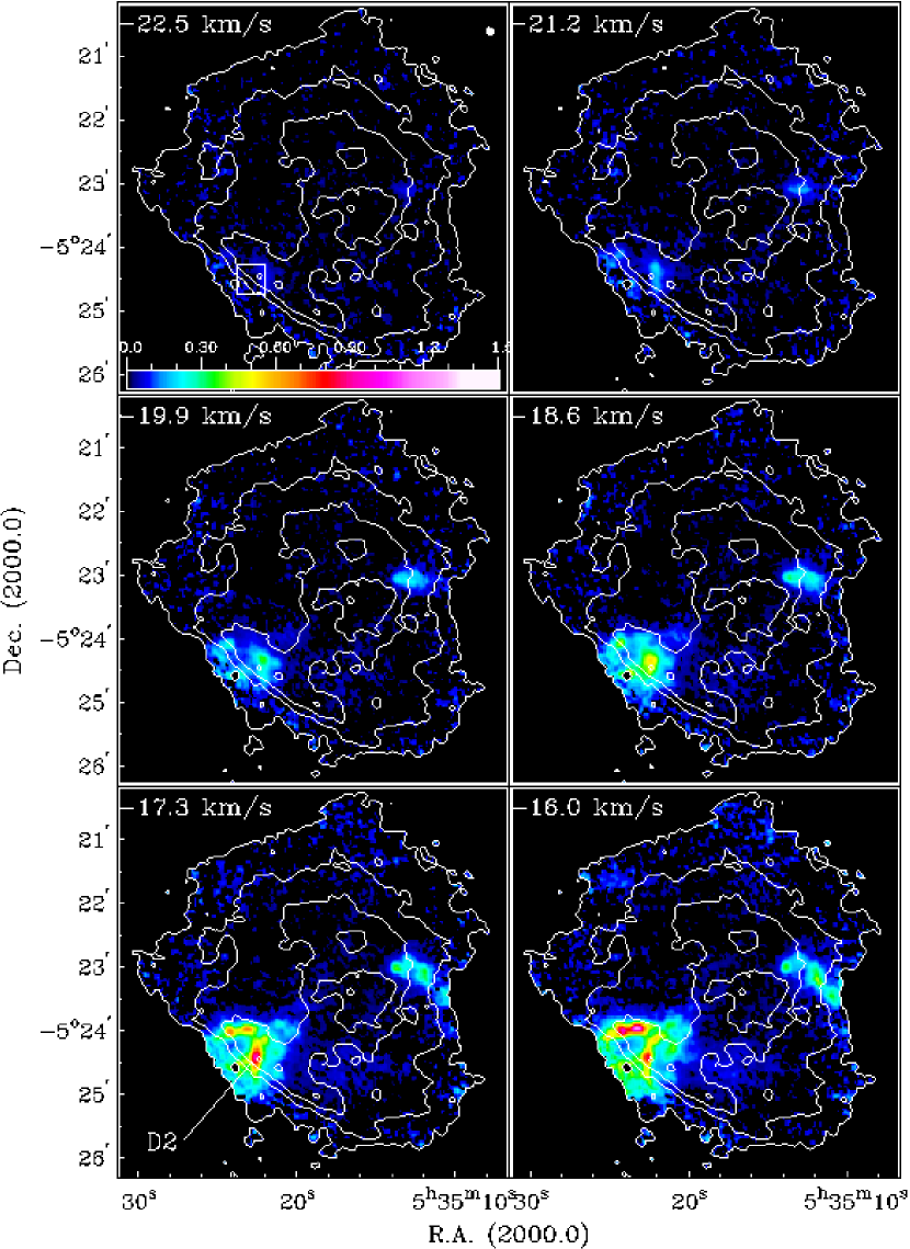
Figure 9.— Images of H i opacity (color images), at the LSR velocities indicated in the upper left-hand corner of each frame. White contours indicate the background $21\;\hbox{\rm cm}$ continuum at levels of 50, 100, 200, 300 and $400\;\hbox{\rm mJy}\;\hbox{\rm beam}^{-1}$. Black pixels within the faintest continuum contour denote positions affected by saturation. The opacity scale is indicated by the color bar in the first frame. In this frame also the region over which the opacity spectrum shown in Fig. 8 has been averaged, is shown. The size and orientation of the synthesized beam (${7^{\prime\prime}\hskip-4.60007pt.\hskip 1.19995pt2}\times{5^{\prime\prime}\hskip-4.60007pt.\hskip 1.19995pt7}$ at a position angle of $29.7^{\circ}\hskip-2.84544pt$) is indicated by the ellipse in the top righthand corner of the first frame. Letters C–M indicate various absorption features discussed in the text.

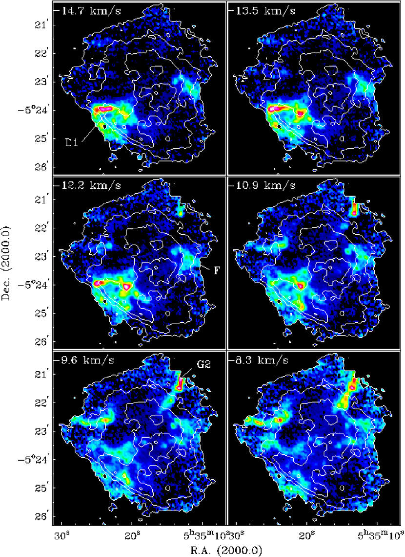
Figure 9.— (continued)

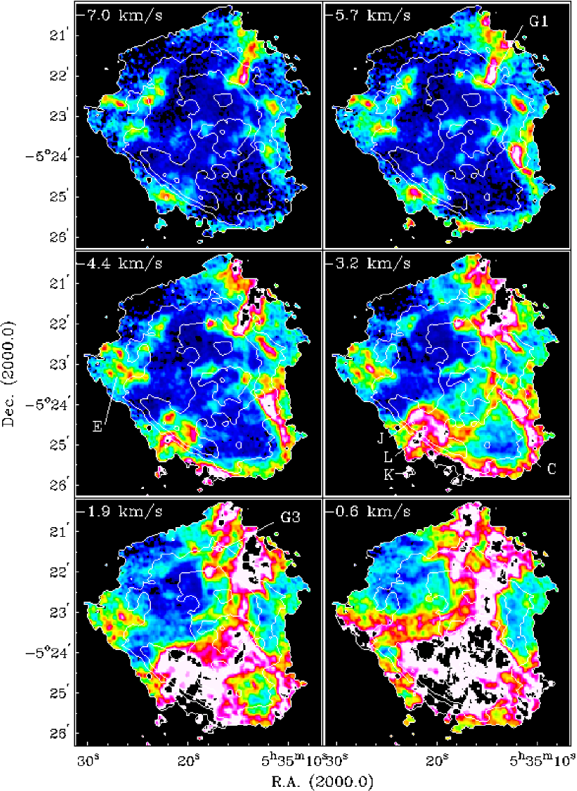
Figure 9.— (continued)

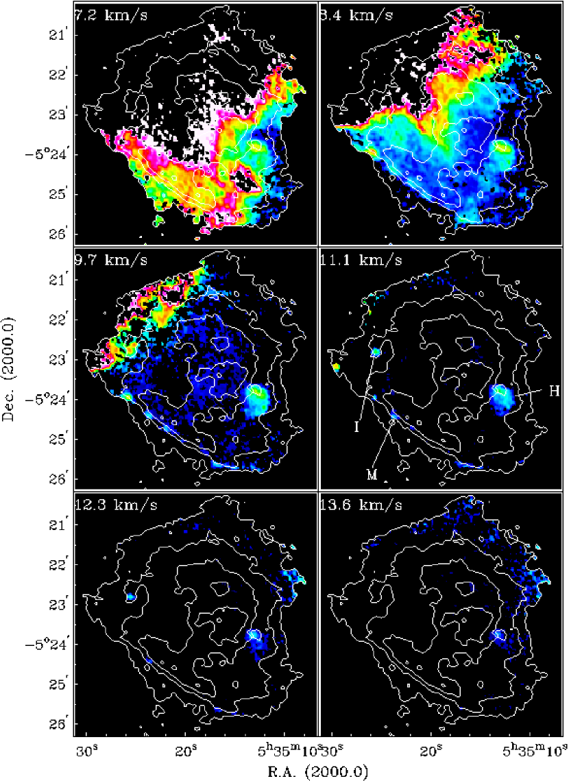
Figure 9.— (continued)

5.2. H i opacity images

In order to study the morphology of the H i opacity as a function of $v_{\rm LSR}$, we present a sequence of opacity images. For presentation purposes, the data cube was spectrally smoothed (ignoring saturated pixels) to a channel resolution and separation of $1.28\;\hbox{\rm km}\;\hbox{\rm s}^{-1}$. A sequence of these images is shown in Fig. 9. We note that the smoothing in velocity was only done for the purpose of creating these figures; all analysis was done on the full velocity resolution data cube. The range $0.6\;\hbox{\rm km}\;\hbox{\rm s}^{-1}<v_{\rm LSR}<5.9\;\hbox{\rm km}\;\hbox{\rm s}^{-1}$ is heavily affected by saturation. Therefore, this region, covering part of component A and most of component B, was omitted from Fig. 9.

5.2.1 Large-scale H i absorption features

We focus first on the components A, B and C identified by vdWG89. Referring to Fig. 8, the red line wing of component A is traced in the opacity image at $v_{\rm LSR}=8.4\;\hbox{\rm km}\;\hbox{\rm s}^{-1}$. A strong increase in opacity is observed towards the Northeast Dark Lane, in agreement with the results of vdWG89.

Component C of vdWG89, located at the southwestern edge of the Huygens region, can be traced in the opacity images between $-4.4$ and $-0.6\;\hbox{\rm km}\;\hbox{\rm s}^{-1}$. The morphology of this component is obvious at $v_{\rm LSR}=-3.2\;\hbox{\rm km}\;\hbox{\rm s}^{-1}$, where it displays a striking arc of high H i opacity tracing the extreme southwest edge of the Huygens region, and broken into a number of H i peaks. Several other H i features are detected in the same velocity range, most notably near the Bright Bar and towards the northern part of Huygens region. However, as will be discussed below (Sects. 5.3.5 and 5.3.6), those features are not physically related to the prominent H i opacity arc at the southwest edge of the Huygens region. Therefore in our nomenclature component  C will only denote this H i arc.

Table 1Global parameters of small-scale H i components

Name	R.A.	Dec.	$v_{\rm LSR}$ range	Diameter		$N(\hbox{{\rm H}}\,\hbox{{\sc i}})\left({T_{\rm s}\over 100\;\hbox{\rm K}}\right)$		$M_{\hbox{{\rm H}}\,\hbox{{\sc i}}}\left({T_{\rm s}\over 100\;\hbox{\rm K}}\right)$	Associated with
	[J2000]		[km s-1]		[pc]	[$10^{19}\;\hbox{\rm cm}^{-2}$]		[$M_{\odot}$]
						peak	mean
D	$5^{\rm h}\,35^{\rm m}\,23^{\rm s}\hskip-3.9pt.\hskip 0.80002pt0$	$-5^{\circ}\,24^{\prime}\,30^{\prime\prime}$	$-21.2\to-10.9$	${1^{\hskip 0.35002pt\prime}\hskip-3.50006pt.\hskip 0.50003pt5}$	0.21	100	6.6	0.07	$\theta^{2}$B Ori
E	$5^{\rm h}\,35^{\rm m}\,25^{\rm s}\hskip-3.9pt.\hskip 0.80002pt0$	$-5^{\circ}\,23^{\prime}\,00^{\prime\prime}$	$-10.9\to-1.9$	${1^{\hskip 0.35002pt\prime}\hskip-3.50006pt.\hskip 0.50003pt5}$	0.21	130	6.2	0.07	Dark Bay
F	$5^{\rm h}\,35^{\rm m}\,14^{\rm s}\hskip-3.9pt.\hskip 0.80002pt0$	$-5^{\circ}\,23^{\prime}\,00^{\prime\prime}$	$-21.2\to-10.9$	$40^{\prime\prime}$	0.09	24	9.2	0.02	${\rm HH}\,{\rm 202}$
G1	$5^{\rm h}\,35^{\rm m}\,14^{\rm s}\hskip-3.9pt.\hskip 0.80002pt0$	$-5^{\circ}\,21^{\prime}\,40^{\prime\prime}$	$-9.6\to-1.9$	${1^{\hskip 0.35002pt\prime}\hskip-3.50006pt.\hskip 0.50003pt5}$	0.21	$>350$	3.6	0.04
G2	$5^{\rm h}\,35^{\rm m}\,13^{\rm s}\hskip-3.9pt.\hskip 0.80002pt0$	$-5^{\circ}\,21^{\prime}\,20^{\prime\prime}$	$-12.2\to-8.3$	$30^{\prime\prime}$	0.07	$>350$	12	0.02	$\hbox{\rm H}_{2}$ finger
G3	$5^{\rm h}\,35^{\rm m}\,17^{\rm s}\hskip-3.9pt.\hskip 0.80002pt5$	$-5^{\circ}\,21^{\prime}\,40^{\prime\prime}$	$-3.2\to-0.6$	${1^{\hskip 0.35002pt\prime}\hskip-3.50006pt.\hskip 0.50003pt5}$	0.21	27	2.7	0.03
H	$5^{\rm h}\,35^{\rm m}\,13^{\rm s}\hskip-3.9pt.\hskip 0.80002pt0$	$-5^{\circ}\,24^{\prime}\,00^{\prime\prime}$	$+7.2\to+12.3$	$40^{\prime\prime}$	0.09	34	9.9	0.02	Orion-S
I	$5^{\rm h}\,35^{\rm m}\,25^{\rm s}\hskip-3.9pt.\hskip 0.80002pt6$	$-5^{\circ}\,22^{\prime}\,49^{\prime\prime}$	$+9.7\to+13.0$	$8^{\prime\prime}$	0.02	23	20	0.002	extinction Knot 2
J	$5^{\rm h}\,35^{\rm m}\,22^{\rm s}\hskip-3.9pt.\hskip 0.80002pt0$	$-5^{\circ}\,24^{\prime}\,52^{\prime\prime}$	$-4.4\to-1.2$	$30^{\prime\prime}$	0.07	$>340$	3.3	0.04	${\rm HH}\,{\rm 203{/}204}$
K	$5^{\rm h}\,35^{\rm m}\,23^{\rm s}\hskip-3.9pt.\hskip 0.80002pt0$	$-5^{\circ}\,25^{\prime}\,45^{\prime\prime}$	$-5.7\to-0.6$	$10^{\prime\prime}$	0.02				shock south of ${\rm HH}\,{\rm 204}$
L	$5^{\rm h}\,35^{\rm m}\,20^{\rm s}\hskip-3.9pt.\hskip 0.80002pt4$	$-5^{\circ}\,24^{\prime}\,25^{\prime\prime}$	$-5.7\to-0.6$	$1^{\prime}$	0.14	$>330$	10	0.05	$\theta^{2}$A Ori
M	$5^{\rm h}\,35^{\rm m}\,25^{\rm s}\hskip-3.9pt.\hskip 0.80002pt8$	$-5^{\circ}\,23^{\prime}\,57^{\prime\prime}$	$+7.8\to+11.7$	$12^{\prime\prime}$	0.03	46	4.5	0.001	Bright Bar

5.2.2 Small-scale H i absorption features

To trace the small-scale H i absorption components, we begin at the most negative velocities and follow the opacity images towards more positive velocities. Central positions and velocity ranges over which these features are detected are summarized in Table 1. The components are also indicated in Figs. 9 and 13. Table 1 also summarizes H i masses, and peak and average column densities, as well as approximate total sizes of the various features. The H i masses and column densities scale with $T_{\rm s}$, here assumed to be $100\;\hbox{\rm K}$ (see Sect. 7.1). For convenience, the formulae relating the H i emission and absorption measurements for H i column densities, and the underlying assumptions, are summarized in the Appendix.

The most negative velocity components in our data are components D (in the region of the Bright Bar) and F (in the western part of the Huygens region). Both are detected over a considerable velocity range ($-21.2<v_{\rm LSR}<-10.9\;\hbox{\rm km}\;\hbox{\rm s}^{-1}$). The more opaque component D displays obvious extended structure with embedded higher opacity clumps. Both components contain several velocity components, in agreement with vdWG90.

Continuing to more positive velocities, component E of vdWG90 is detected in the region of the Dark Bay. The data shown by vdWG90 already indicated that this component consists of several clumps, which are more prominent in the present higher resolution data. Inspection of Fig. 9 in the region of component E reveals the presence of 10 compact H i opacity clumps. At the resolution of $\sim 6^{\prime\prime}$, the diameters of the unresolved clumps are less than $0.014\;\hbox{\rm pc}$ or $2800\;\hbox{\rm AU}$.

The remaining blueshifted small-scale feature identified by vdWG90, component G, is detected as a conspicuous elongated feature towards the northern part of M42 at velocities from $-4$ to $-11\;\hbox{\rm km}\;\hbox{\rm s}^{-1}$.

One compact feature was identified by vdWG90 at positive $v_{\rm LSR}$ (their component H). This feature is at the velocity of OMC-1 and it is detected at $v_{\rm LSR}=7-12\;\hbox{\rm km}\;\hbox{\rm s}^{-1}$ in Fig. 9 in the western part of the Huygens region.

The data cube was carefully searched for additional velocity components. No additional H i components were found at velocities more negative than that of component D, even though Na i and Ca ii absorption line measurements towards the Trapezium stars and $\theta^{2}$ A Ori reveal several of components at these velocities, e.g., at $v_{\rm LSR}\approx-32.8$, $-20.6$, $-17.0$, and $-12.1\;\hbox{\rm km}\;\hbox{\rm s}^{-1}$ (O’Dell et al., 1993). Likewise, no absorption was found at velocities more positive than that of component H. However, our search revealed several new small-scale features within the velocity range shown in Fig. 9, spatially and kinematically distinct from the features described above. Some of these features are quite compact, or are located close to other features, which accounts for their non-detection in the lower resolution data of vdWG90. Several features are quite close in velocity to component C, but spectra and position-velocity diagrams reveal that these features are kinematically distinct. Their global properties are summarized in Table 1. These features are best seen in PV diagrams discussed below.

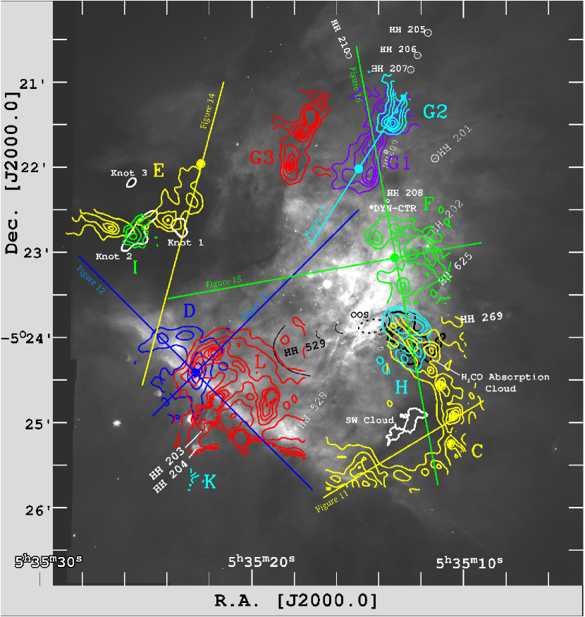
Figure 13.— Location of the position-velocity (PV) diagrams of H i optical depth shown in Figs. 14–20, superposed on an HST/WFPC2 image (greyscale). The lengths, orientations and positions of these PV diagrams are indicated by the colored bars. In each bar, a thick dot of the same color indicates the zero position of the spatial coordinate in the corresponding PV diagram. Finally, contour sets indicate the H i opacity of the various H i features shown in Figs. 14–20. These contours are taken from the opacity images at $-2.5\;\hbox{\rm km}\;\hbox{\rm s}^{-1}$ (yellow contours in southwest, indicating component C, and red contours near the Bright Bar, indicating components J and L); $-17.3\;\hbox{\rm km}\;\hbox{\rm s}^{-1}$ (dark blue contours near the Bright Bar, indicating component D, and green contours indicating component F); $-7.0\;\hbox{\rm km}\;\hbox{\rm s}^{-1}$ (yellow, component E); $-7.7\;\hbox{\rm km}\;\hbox{\rm s}^{-1}$ (purple contours in northwest, indicating component G1); $-9.6\;\hbox{\rm km}\;\hbox{\rm s}^{-1}$ (light blue, component G2); $-1.3\;\hbox{\rm km}\;\hbox{\rm s}^{-1}$ (red contours in the north, indicating component G3); $8.4\;\hbox{\rm km}\;\hbox{\rm s}^{-1}$ (light blue contours southwest of the Trapezium stars, indicating component H); $10.3\;\hbox{\rm km}\;\hbox{\rm s}^{-1}$ (green, component I); and $1.9\;\hbox{\rm km}\;\hbox{\rm s}^{-1}$ (light blue contours in the south, indicating component K). The optical HST image is a combination of the WFPC2 F502N and F658N filter images from O’Dell & Wong (1996), which contain respectively the [O iii] $5007\;\hbox{\rm\AA}$ and the [N ii] $6583\;\hbox{\rm\AA}$ and $\hbox{{\rm H}}\alpha$ lines, thus the extremes of both high and low excitation levels. The features indicated by “SW Cloud” and “Knot 1$-$3” are features of enhanced extinction identified in the extinction study of O’Dell & Yusef-Zadeh (2000). “Dyn-ctr” indicates the dyanmical center of the Orion-KL molecular outflow, discussed further in Sect. 6.3. “$\hbox{\rm H}_{2}\hbox{\rm CO}$ absorption cloud” denotes the outline of the $\hbox{\rm H}_{2}\hbox{\rm CO}$ absorption signal of Orion-S. The optical outflow source associated with Orion-S is indicated by “OOS”. These features are discussed in Sect. 7.5.1.

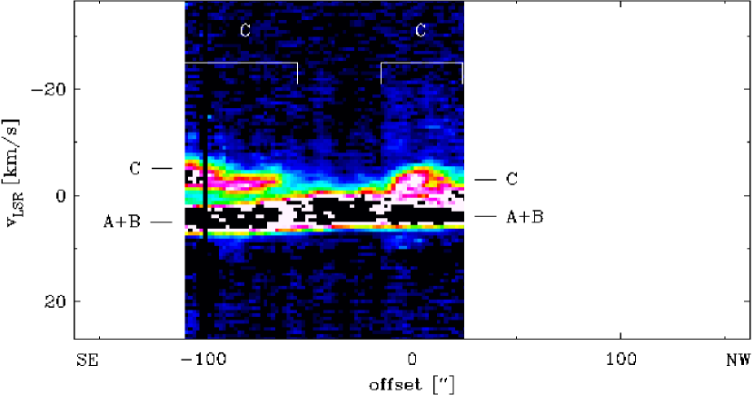
Figure 14.— Position-velocity diagram of H i optical depth along the yellow southeast-northwest bar shown in Fig. 13 towards the southwest of the Huygens region. The spatial axis has its zero position at $\hbox{\rm RA}=5^{\rm h}\,35^{\rm m}\,10^{\rm s}\hskip-3.9pt.\hskip 0.80002pt5$, $\hbox{\rm Dec}=-5^{\circ}\,24^{\prime}\,56^{\prime\prime}$ and a position angle of $120^{\circ}\hskip-2.84544pt$. Spatial offsets are negative towards the southeast and positive towards the northwest. Velocity components discussed in the text are indicated.

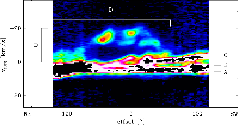
Figure 15.— Position-velocity diagram of H i optical depth along the dark blue northeast-southwest bar shown in Fig. 13. The spatial axis has its zero position at $\hbox{\rm RA}=5^{\rm h}\,35^{\rm m}\,22^{\rm s}\hskip-3.9pt.\hskip 0.80002pt6$, $\hbox{\rm Dec}=-5^{\circ}\,24^{\prime}\,25^{\prime\prime}$ and a position angle of $45^{\circ}\hskip-2.84544pt$. Spatial offsets are negative towards the northeast and positive towards the southwest. Velocity components discussed in the text are indicated.

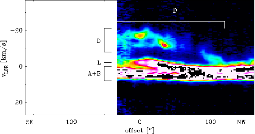
Figure 16.— Position-velocity diagram of H i optical depth along the dark blue southeast-northwest bar shown in Fig. 13. The spatial axis has the same zero position as for Fig. 15, but has a position angle of $135^{\circ}\hskip-2.84544pt$, perpendicular to the PV diagram shown in Fig. 15. Spatial offsets are negative towards the southeast and positive towards the northwest. Velocity components discussed in the text are indicated.

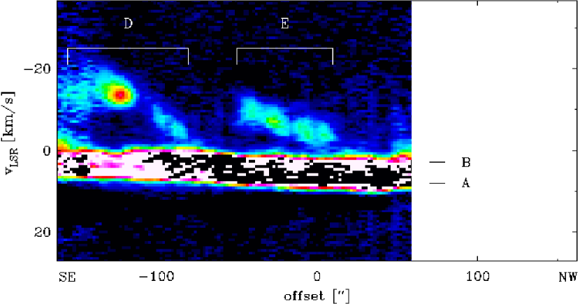
Figure 17.— Position-velocity diagram of H i optical depth along the yellow southeast-northwest bar west of the Trapezium stars, shown in Fig. 13. The spatial axis has its zero position at $\hbox{\rm RA}=5^{\rm h}\,35^{\rm m}\,22^{\rm s}\hskip-3.9pt.\hskip 0.80002pt4$, $\hbox{\rm Dec}=-5^{\circ}\,21^{\prime}\,58^{\prime\prime}$ and a position angle of $345^{\circ}\hskip-2.84544pt$. Spatial offsets are negative towards the southeast and positive towards the northwest. Velocity components discussed in the text are indicated.

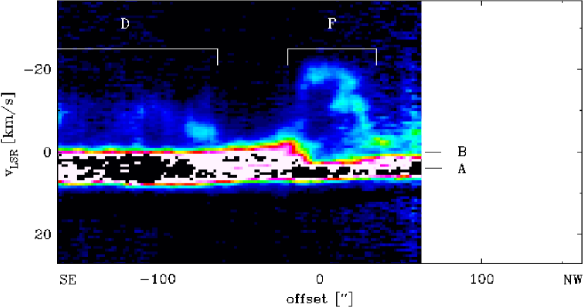
Figure 18.— Position-velocity diagram of H i optical depth along the green southeast-northwest bar shown in Fig. 13. The spatial axis has its zero position at $\hbox{\rm RA}=5^{\rm h}\,35^{\rm m}\,13^{\rm s}\hskip-3.9pt.\hskip 0.80002pt2$, $\hbox{\rm Dec}=-5^{\circ}\,23^{\prime}\,04^{\prime\prime}$ and a position angle of $100^{\circ}\hskip-2.84544pt$. Spatial offsets are negative towards the southeast and positive towards the northwest. Velocity components discussed in the text are indicated.

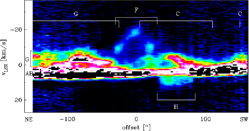
Figure 19.— Position-velocity diagram of H i optical depth along the green northeast-southwest bar shown in Fig. 13. The spatial axis has the same zero position as for Fig. 18, but has a position angle of $10^{\circ}\hskip-2.84544pt$, perpendicular to the PV diagram shown in Fig. 18. Spatial offsets are negative towards the northeast and positive towards the southwest. Velocity components discussed in the text are indicated.

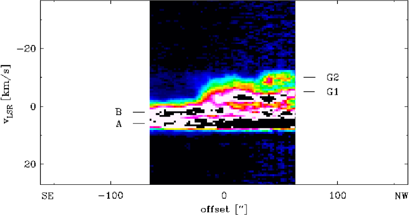
Figure 20.— Position-velocity diagram of H i optical depth along the light blue southeast-northwest bar shown in Fig. 13. The spatial axis has its zero position at $\hbox{\rm RA}=5^{\rm h}\,35^{\rm m}\,14^{\rm s}\hskip-3.9pt.\hskip 0.80002pt9$, $\hbox{\rm Dec}=-5^{\circ}\,22^{\prime}\,01^{\prime\prime}$ and a position angle of $328^{\circ}\hskip-2.84544pt$. Spatial offsets are negative towards the southeast and positive towards the northwest. Velocity components discussed in the text are indicated.

5.3. Position-velocity diagrams of H i opacity

The location of a set of illustrative PV diagrams is indicated in Fig. 13. These diagrams are presented in Figs. 14–20. The various H i components are indicated in these figures.

5.3.1 Components A, B and C

Figure 14 shows the saturated signal of the large-scale components A and B at positive velocities. In addition, component C is detected at slightly negative velocities ($-4$ to $-2\;\hbox{\rm km}\;\hbox{\rm s}^{-1}$). As already indicated by the channel map at $-3.2\;\hbox{\rm km}\;\hbox{\rm s}^{-1}$, Fig. 14 shows that this component does not cover the entire nebula (in contrast to components A and B), but is found only at the edge of the Huygens region, where it forms a large arc in the shape of an incomplete semicircle.

5.3.2 Structure and extent of component D

The velocity structure and extent of the most extended small-scale component D is shown in Figs. 15 and 16, which show crosscuts through this feature in orthogonal directions. Figure 15, which shows a PV diagram approximately along the Bright Bar, shows that this component is extended over about $160^{\prime\prime}$. The prominent high opacity features seen at the most negative velocities appear to be connected to the main H i components through gas at intermediate velocities. Inspection of Fig. 16, which presents a PV diagram roughly perpendicular to the Bright Bar, shows a velocity gradient, in the sense that the most negative velocities occur to the southeast. The overall velocity structure therefore resembles that of an expanding shell. This impression is reinforced by the morphology of the absorbing H i, in particular at velocities between $-17.3$ and $-10.9\;\hbox{\rm km}\;\hbox{\rm s}^{-1}$, and also illustrated by the dark blue contours in Fig. 13. Figure 16 also shows that the blueshifted gas of component D connects to the larger scale H i layers through gas at intermediate velocities, located approximately $20^{\prime\prime}$ east of the Trapezium stars.

5.3.3 Component E: H i in the Dark Bay

A PV diagram through component E, which is located in the area of the Dark Bay, is shown in Fig. 17. While this component is resolved into a number of compact opacity peaks, these are obviously part of one coherent velocity structure. This diagram also demonstrates that although in projection components D and E are almost contiguous, component E is actually a kinematically separate feature.

5.3.4 Stucture of the high velocity component F

The PV diagrams of the high velocity component F in Figs. 18 and 19 reveal clearly that the high (negative) velocity gas is connected with the main H i components through features at intermediate velocities. This is particularly clear in Fig. 18, where the high velocity gas (which shows several velocity components) is connected to the lower velocity gas through a prominent H i feature at its northwestern side. Careful inspection of Fig. 18 and of the H i opacity data cube reveals that a fainter connection between the high velocity gas and the large-scale components is also present at the southeast side of the feature.

The fact that the location of component F spatially coincides with a gap in the extended gas layer at less negative velocities is striking. This behavior argues that component F is physically part of the larger scale H i layer, but that it has been accelerated to negative velocities. The situation is further illustrated by Fig. 19, which shows a PV diagram along a position angle perpendicular to Fig. 18. The connection with the lower velocity gas is clearly observed on both sides of the feature, as well as the gap in less negative velocity gas at the position component F.

Like component D, the velocity structure of component F resembles that of an expanding bubble or shell, although this interpretation ignores the fact that at some positions several velocity components are present. However, component F is much more confined than component D, with a diameter of about $60^{\prime\prime}$ ($0.14\;\hbox{\rm pc}$).

5.3.5 The elongated component G

A PV diagram over the long axis of the elongated component G is shown in Fig. 20. Inspection of the line images in Fig. 9 shows that multiple elongated H i absorption features are present towards the northern part of M42 at the full velocity range from $-0.6$ to $-12.2\;\hbox{\rm km}\;\hbox{\rm s}^{-1}$, which we collectively denote component G. The PV diagram in Fig. 20 shows a prominent feature at velocities of $-3$ to $-4\;\hbox{\rm km}\;\hbox{\rm s}^{-1}$. However, at more negative velocities (approximately $-10\;\hbox{\rm km}\;\hbox{\rm s}^{-1}$), an additional feature is detected towards the northern part of the nebula. We denote the features at $\sim-3\;\hbox{\rm km}\;\hbox{\rm s}^{-1}$ G1 and the feature at $\sim-10\;\hbox{\rm km}\;\hbox{\rm s}^{-1}$ G2, as indicated in Fig. 20. The latter feature matches component G of vdWG90. Finally, we note that a parallel and similarly elongated H i absorption feature appears $\sim 45^{\prime\prime}$ east of component G1 at velocities of $-1.9$ and $-0.6\;\hbox{\rm km}\;\hbox{\rm s}^{-1}$ in Fig. 9; we denote the eastern feature component G3.

5.3.6 The arclike component L

At $v_{\rm LSR}=-3.2\;\hbox{\rm km}\;\hbox{\rm s}^{-1}$ in Fig. 9, a prominent absorption feature is detected at approximately the location of the Bright Bar. This feature, indicated by red contours in Fig. 13, was included by vdWG89 in component C, based on the agreement in velocity. The higher resolution provided by the present data however shows that this feature is distinct from component C, as will be discussed in Sect. 7.2. This feature, which we denote by L, has an arc-like structure, open towards the southeast, similar to the shape of component D (indicated by dark blue contours in Fig. 13). It reveals a velocity gradient with more negative velocities towards the southeast (e.g., Fig. 16), similar to component D.

5.3.7 The elongated component J

Southeast of component L, and at approximately the same velocity ($\sim-3\;\hbox{\rm km}\;\hbox{\rm s}^{-1}$), an elongated H i feature is found in the opacity images, crossing the Bright Bar orthogonally. A PV diagram through this feature, which we label J, shows that it is kinematically distinct from component L, and at slightly more negative velocities. Component J is similar to component G in appearing elongated, and has a velocity gradient oriented along its long axis.

5.3.8 Component K

A compact absorption feature at $\sim-3.2\;\hbox{\rm km}\;\hbox{\rm s}^{-1}$, which we label component K, is detected in Fig. 9 south of component J.

5.3.9 Features at the velocity of OMC-1

Several features at the velocity of the background molecular cloud OMC-1 are found in the present data. Component H was already discovered by vdWG90 and is detected as an extended feature in Fig. 9 at $7.2-11.1\;\hbox{\rm km}\;\hbox{\rm s}^{-1}$, and in the PV diagram in Fig. 19. In addition, a system of compact features is found directly southeast of the Bright Bar and most likely associated with it. These features can be seen in Fig. 9, at a velocity of $9.7\;\hbox{\rm km}\;\hbox{\rm s}^{-1}$, and we denote them collectively as component M. The most prominent of these is located at the extreme eastern edge of the Bright Bar at $\hbox{\rm RA}=5^{\rm h}\,35^{\rm m}\,25^{\rm s}\hskip-3.9pt.\hskip 0.80002pt8$, $\hbox{\rm Dec}=-5^{\circ}\,23^{\prime}\,57^{\prime\prime}$. Following the Bright Bar towards the southwest, several similar features are detected. One of these components can be seen in the sample spectrum shown in Fig. 8 and the H i emission PV diagram shown in Fig. 6.

In the Dark Bay region, a single compact H i absoption feature is found at the velocity of OMC-1. This component (component I) can clearly be seen in the opacity images at $11.1$ and $12.3\;\hbox{\rm km}\;\hbox{\rm s}^{-1}$. It was also shown in the PV diagram of H i emission in Fig. 7.

6. H i emission associated with the Orion Nebula

The H i emission images and PV diagrams presented in Sect. 4 show a number of separate features revealing the neutral environment of the Orion Nebula and the effects of H ii region and the ONC on this environment.

1. H i emission at approximately the velocity of the main absorbing components A and B is detected in regions where strong absorption is absent. This layer, which is shown in the PV diagrams in Figs. 4–6, contains a bright H i emission feature, detected in Fig. 4 at a spatial offset of appoximately $150^{\prime\prime}$ This feature is therefore located between M42 and M43 and may represent photodissociated gas outside an IF bounding M42 on the side of the Northeast Dark Lane. This region lies immediately northeast of sample 5-east in O’Dell & Harris (2010). Their Figure 1 shows that this region corresponds to an overlap of a northern protusion from the Dark Bay and the Northeast Dark Lane. Since H i emission could arise from both features, it is impossible to unambiguously assign the observed emission.

2. A prominent H i emission feature is detected in Fig. 2 southeast of the Bright Bar, i.e., the Orion Bar PDR. As shown in Figs. 2 and 5, an elongated H i emission system extends from this feature towards the southwest at $v_{\rm LSR}\sim 14\;\hbox{\rm km}\;\hbox{\rm s}^{-1}$ along.

3. High-velocity H i emission arising from a small region is seen at $v_{\rm LSR}\sim 18\;\hbox{\rm km}\;\hbox{\rm s}^{-1}$ in Fig. 2 and in the PV diagrams in Figs. 6 and 7.

4. H i emission is detected from the Dark Bay region, and this feature is centered on the H i absorption component I, as shown in Fig. 7.

Figure 21.— Spectrum of H i brightness temperature $T_{\rm b}$, averaged over a $45^{\prime\prime}\times 36^{\prime\prime}$ rectangular region parallel to the Bright Bar (position angle $55^{\circ}\hskip-2.84544pt$), centered on RA=$5^{\rm h}\,35^{\rm m}\,21^{\rm s}\hskip-3.9pt.\hskip 0.80002pt3$, Dec=$-5^{\circ}\,25^{\prime}\,08^{\prime\prime}$. This region is indicated by a yellow rectangle in Fig. 3.

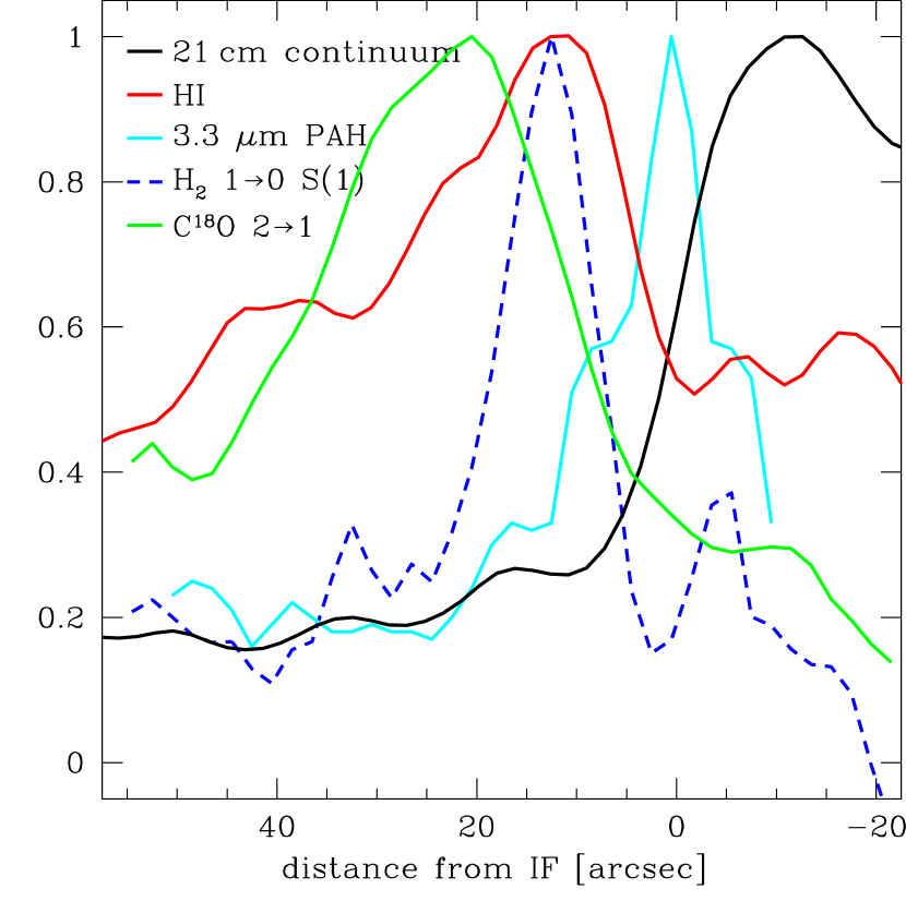
Figure 22.— Normalized crosscuts across the Bright Bar and the Orion Bar PDR in various tracers. The crosscuts cover a length of $75^{\prime\prime}$ perpendicular to the Bar at a position angle of $145^{\circ}\hskip-2.84544pt$, and have been averaged parallel to the bar over a strip with a total width of $45^{\prime\prime}$. The center of this strip passes through coordinates $\hbox{\rm RA}=5^{\rm h}\,35^{\rm m}\,21^{\rm s}\hskip-3.9pt.\hskip 0.80002pt3$, $\hbox{\rm Dec}=-5^{\circ}\,25^{\prime}\,08^{\prime\prime}$, i.e., the central position for the spectrum shown in Fig. 21. The location of this strip is shown by a purple rectangle in Fig. 3, and it is identical to that used by Van der Werf et al. (1996) to construct their Fig. 9. The abscissa shows distance (positive towards the southeast) from the IF, where the 0 position has been chosen as the point of maximum $3.3\;\mu\hbox{\rm m}$ PAH emission, which marks the location of the IF. The $21\;\hbox{\rm cm}$ continuum and H i brightness temperature data are from the present paper, while the $3.3\;\mu\hbox{\rm m}$ PAH data are from Tielens et al. (1993) and Bregman et al. (1994). The $\hbox{\rm H}_{2}$ $v=1{-}0$ S(1) and $\hbox{\rm C}^{18}\hbox{\rm O}$ $2{-}1$ data are from Van der Werf et al. (1996).

6.1. H i emission from the Orion Bar PDR

The brightest H i emission in Fig. 2 is found directly southeast of the Bright Bar, thus arising in the prominent edge-on PDR. An H i emission spectrum, averaged over the region shown by the yellow box in Fig. 3, is shown in Fig. 21. This spectrum is very similar to the H i spectrum of this region obtained almost 40 years earlier with the Parkes $64\;\hbox{\rm m}$ telescope shown in Fig. 6 of Radhakrishnan et al. (1972).

Our observation of H i emission from the Orion Bar probes a significantly younger PDR, with much higher gas density than previous studies of PDRs associated with evolved H ii regions such as ${\rm NGC}\,{\rm 281}$ (Roger & Pedlar, 1981), ${\rm NGC}\,{\rm 1579}$ (Dewdney & Roger, 1982, 1986), ${\rm IC}\,{\rm 5146}$ (Roger & Irwin, 1982), S187 (Joncas et al., 1992), S185 (which contains the well-studied PDR ${\rm IC}\,{\rm 63}$ Blouin et al., 1997) and S270 (Roger et al., 2004). Due to the high resolution and the edge-on orientation of the Orion Bar, our observations offer for the first time the opportunity to use H i to study the stratified structure of such a PDR. We therefore construct a crosscut perpendicular to the bar in various tracers, as shown in Fig. 22). This figure dramatically confirms the layered structure of the PDR, and for the first time observationally pinpoints the location of atomic hydrogen in a resolved edge-on PDR. The edge-on IF is marked by the peak in $3.3\;\mu\hbox{\rm m}$ PAH emission, which is strongly excited in the neutral UV-exposed layer directly outside the IF (Tielens et al., 1993; Kassis et al., 2006).

The most important parameter in determining the thickness of a homogeneous PDR and therefore the separation of the various tracers in Fig. 22 is the dissociation parameter $\chi/n_{\hbox{\scriptsize\rm H}}$ (e.g., Tielens & Hollenbach, 1985b; Sternberg, 1988; Burton et al., 1990; Draine & Bertoldi, 1996; Hollenbach & Tielens, 1999), where $\chi$ represents the intensity of the incident UV radiation field, and $n_{\hbox{\scriptsize\rm H}}$ is the number density of hydrogen nuclei. The structure can be modified if the gas is clumpy (Burton et al., 1990; Meixner & Tielens, 1993; Tauber et al., 1994; Young Owl et al., 2000), since in this case UV photons penetrate deeper into the cloud through the interclump medium (e.g., Boisse, 1990). For the Orion Bar PDR, the incident UV radiation field at the IF is $\chi=2.6\times 10^{4}$, where $\chi$ is expressed in units of the Draine (1978) interstellar radiation field of $2.7\times 10^{-3}\;\hbox{\rm erg}\;\hbox{\rm s}^{-1}\;\hbox{\rm cm}^{-2}$. This value of $\chi$ was derived directly from the properties of the Trapezium stars and their distance from the Bright Bar (Tielens & Hollenbach, 1985a). Analysis of the stratified structure then yields a gas density $n_{\hbox{\scriptsize\rm H}}=1-2\times 10^{5}\;\hbox{\rm cm}^{-3}$, (Tielens et al., 1993; Simon et al., 1997; Van der Wiel et al., 2009), with higher density (up to $n_{{\hbox{\scriptsize H}}_{2}}=10^{7}\;\hbox{\rm cm}^{-3}$) embedded clumps (Tauber et al., 1994; Van der Werf et al., 1996; Young Owl et al., 2000; Lis & Schilke, 2003). We now discuss our H i observations of the Orion Bar in the context of this model.

As shown in Fig. 21, the peak H i brightness temperature in the Orion Bar PDR is approximately $230\;\hbox{\rm K}$, and the H i spin temperature and kinetic temperature are therefore at least this high. Such temperatures are easily reached in PDRs exposed to an intense UV radiation field. For the values of $\chi$ and $n_{{\hbox{\scriptsize H}}_{2}}$ applicable to the Orion Bar, PDR models predict gas kinetic temperatures of approximately $1000\;\hbox{\rm K}$ at the UV-exposed surface (Le Petit et al., 2006; Meijerink et al., 2007; Kaufman et al., 1999), decreasing to values of a few hundred K at larger distances ($>0.01\;\hbox{\rm pc}$) from the IF. An upper limit for the kinetic temperature follows from the observed linewidth, using

$$\Delta v_{\rm FWHM}=2\sqrt{2\ln 2{kT_{\rm kin}\over m_{\hbox{\scriptsize\rm H\,\sc I}}}},$$ (2)

where $m_{\hbox{\scriptsize\rm H\,\sc I}}$ is the mass of the H i atom. While the low velocity side of the emission feature in Fig. 21 may be affected by absorption, the high velocity side appears to be unaffected, and at that side the HWHM of the line is $2.6\;\hbox{\rm km}\;\hbox{\rm s}^{-1}$, corresponding to a FWHM of $5.2\;\hbox{\rm km}\;\hbox{\rm s}^{-1}$. This line width implies tha $T_{\rm s}<590\;\hbox{\rm K}$. The turbulent linewidth in this region, as measured from the optically thin $\hbox{\rm C}^{17}\hbox{\rm O}$ $3{-}2$ line (Johnstone et al., 2003) is $1.3\;\hbox{\rm km}\;\hbox{\rm s}^{-1}$. Allowing for this turbulent velocity gives a thermal FWHM of $5.0\;\hbox{\rm km}\;\hbox{\rm s}^{-1}$, implying $T_{\rm kin}=540\;\hbox{\rm km}\;\hbox{\rm s}^{-1}$. Since the peak brightness temperature is $230\;\hbox{\rm K}$, the implied peak optical depth is $\tau_{0}=0.6$, so the H i line emission is only marginally optically thin. The implied H i column density is $N(\hbox{{\rm H}}\,\hbox{{\sc i}})=3\times 10^{21}\;\hbox{\rm cm}^{-2}$, averaged over the region used to construct Fig. 21. The line of sight molecular hydrogen column density in the bar is $N(\hbox{\rm H}_{2})\approx 6.8\times 10^{22}\;\hbox{\rm cm}^{-2}$ (Hogerheijde et al., 1995; Jansen et al., 1995; Van der Werf et al., 1996; Van der Wiel et al., 2009), so that only about 2% of all hydrogen nuclei are in atomic form. Since the dense clumps in the PDR will likely remain molecular, it is more appropriate to consider only the interclump medium with $n_{\hbox{\scriptsize\rm H}}=1-2\times 10^{5}\;\hbox{\rm cm}^{-3}$ for calculating the local H i abundance. The line-of-sight depth of the IF in the Bar region is approximately $0.12\;\hbox{\rm pc}$, as derived from modeling by Pellegrini et al. (2009). Using these numbers, the H i abundance in the Bar is $5-10\%$ at the position of the H i peak.

The derived atomic fraction indicates that the observed H i emission originates in the region where the transition towards molecular gas occurs. This conclusion is supported by the $\hbox{\rm H}_{2}$ temperature in this region from rotational lines, which is $400-700\;\hbox{\rm K}$ (Allers et al., 2005; Shaw et al., 2009), in excellent agreement with our estimate of $540\;\hbox{\rm K}$ for the H i.

Inspection of Fig. 22 reveals strong H i emission from the region where $\hbox{\rm H}_{2}$ vibrational line emission shows a maximum. This agreement is physically significant. Direct $\hbox{\rm H}_{2}$ photodissociation from the ground state is strongly forbidden, since the molecule is homonuclear. The actual photodissociation of $\hbox{\rm H}_{2}$ is a two-step process, initiated by the absorption of UV photons in the Lyman or Werner bands, as first proposed in 1965 by Solomon (private communication in Field et al., 1966). The UV absorption is followed by a radiative cascade, in which there is an 11% chance of dissociation (Stecher & Williams, 1967). In the remaining 89% of cases the molecule cascades down to the ground state, and the resulting fluorescent photon emission produces the $\hbox{\rm H}_{2}$ vibrational lines (Black & Van Dishoeck, 1987; Sternberg, 1988; Sternberg & Dalgarno, 1989, e.g.,). The strong H i emission from the region of maximum $\hbox{\rm H}_{2}$ vibrational line emission therefore directly supports the photodissociation mechanism, and our data reveal this agreement for the first time.

At larger distances from the IF, the H i brightness temperature decreases slowly. The optically thin $\hbox{\rm C}^{18}\hbox{\rm O}$ $J=2{-}1$ emission peaks at a larger distance from the IF than the H i emission ($21^{\prime\prime}$ or $0.05\;\hbox{\rm pc}$). The brightest H i emission is thus located in the region where CO is photodissociated. In this region the gas-phase carbon is singly ionized, and detected through the [C ii] $158\;\mu\hbox{\rm m}$ fine structure line (Stacey et al., 1993; Herrmann et al., 1997) and recombination lines in the radio (Jaffe & Pankonin, 1978; Natta et al., 1994; Wyrowski et al., 1997) and in the near-infrared (Walmsley et al., 2000). The slower decrease of the H i brightness temperature towards larger distances from the IF compared to $\hbox{\rm H}_{2}$ $v=1{-}0$ S(1) results from the fact that collisional excitation contributes to the flux of this $\hbox{\rm H}_{2}$ line (Van der Werf et al., 1996). Observations of the fainter $\hbox{\rm H}_{2}$ $v=2{-}1$ S(1) line, which is dominated by UV-pumped fluorescence reveal a slower decline from the IF (Hayashi et al., 1985; Van der Werf et al., 1996; Luhman et al., 1998; Marconi et al., 1998; Walmsley et al., 2000), matching the decreasing H i brightness temperature in the same region.

The Orion Bar arises from an escarpment protruding from the OMC-1 molecular cloud towards the observer. Southeast of the Bright Bar the IF curves back to a more face-on aspect (Wen & O’Dell, 1995). This geometry is illustrated schematically for instance in Fig. 3 of Pellegrini et al. (2009) and Fig. 13 of O’Dell & Harris (2010). The present H i emission results show that the northeast-southwest extent of this escarpment is much larger than the length of the bright IF in the Huygens region. As the highly elongated H i emission feature at $v_{\rm LSR}=14.9\;\hbox{\rm km}\;\hbox{\rm s}^{-1}$ (Fig. 2) shows, the escarpment extends significantly beyond the Bright Bar towards the southwest. This H i emission feature can be seen as a separate velocity component at $v_{\rm LSR}\sim 15\;\hbox{\rm km}\;\hbox{\rm s}^{-1}$ in Fig. 5, extending over about $11^{\prime}$ ($1.5\;\hbox{\rm pc}$). This H i feature is located in the EON, which is much less well studied than the bright Huygens region. The extended H i feature has a counterpart in a similarly extended feature observed in $8\;\mu\hbox{\rm m}$ emission using IRAC on the Spitzer Space Telescope, representing emission from PAHs at 7.6, 7.8 and $8.6\;\mu\hbox{\rm m}$. An IF bounding the elongated H i feature on its northern side is detected in the wide-field optical images of the Orion Nebula obtained with ACS/HST (Henney et al., 2007). This geometry confirms that the Orion Bar PDR, and thus the escarpment from OMC-1, extends significantly beyond the bright section in the Huygens Region.

Southeast of the brightest section of the Orion Bar PDR the IF curves back to a more face-on aspect (Wen & O’Dell, 1995; Hogerheijde et al., 1995; Jansen et al., 1995; Pellegrini et al., 2009; Ascasibar et al., 2011). A recent Spitzer IRS study has revealed [Ne iii] $15.56\;\mu\hbox{\rm m}$ and other ionized gas lines out to $12^{\prime}$ southeast of the Trapezium stars, i.e., far beyond the Bright Bar (Rubin et al., 2011). Our data reveal an extended H i cloud in this region with a central velocity $v_{\rm LSR}\sim 13\;\hbox{\rm km}\;\hbox{\rm s}^{-1}$. This feature may represent atomic gas in the extended PDR with a more face-on aspect here than in the bright Bar region. All details of the geometry of the Orion Bar region are represented in the diagram shown in the upper panel of Fig. 13 of O’Dell & Harris (2010).

6.2. H i emission from the Dark Bay region

The H i emission images in Fig. 2 also reveal a $\sim 45^{\prime\prime}$ diameter H i emission feature at velocities up to $17\;\hbox{\rm km}\;\hbox{\rm s}^{-1}$ located in the Dark Bay area. The peak of this feature is at $\hbox{\rm RA}=5^{\rm h}\,35^{\rm m}\,24^{\rm s}\hskip-3.9pt.\hskip 0.80002pt0$, $\hbox{\rm Dec}=-5^{\circ}\,22^{\prime}\,30^{\prime\prime}$ at $14.9\;\hbox{\rm km}\;\hbox{\rm s}^{-1}$; the feature extends towards the southeast where it crosses the compact H i absorption feature I at $\hbox{\rm RA}=5^{\rm h}\,35^{\rm m}\,25^{\rm s}\hskip-3.9pt.\hskip 0.80002pt4$, $\hbox{\rm Dec}=-5^{\circ}\,22^{\prime}\,38^{\prime\prime}$. Given the excellent agreement both in velocity and position, as shown in Fig. 7, the emission and absorption feature are almost certainly physically related.

Given that the continuum brightness temperature of the H ii region in this area is $T_{\rm c}\sim 1500\;\hbox{\rm K}$, the emitting H i must be located behind the ionized gas, and is therefore not associated with the Dark Bay, which represents a tongue of absorption in front of the H ii region, with a velocity $v_{\rm LSR}\sim 6\;\hbox{\rm km}\;\hbox{\rm s}^{-1}$ as measured from radio recombination lines of partly ionized gas (Jaffe & Pankonin, 1978).

The H i emission in the Dark Bay area is located east of the region where the IF curves to a more edge-on orientation, as shown by Wen & O’Dell (1995). This location suggests a geometry analogous to that of the Bright Bar, discussed in Sect. 6.1. This idea is supported by the presence of a ${}^{13}\hbox{\rm CO}$ $J=3{-}2$ emission feature in this region, approximately coinciding in orientation and extent with the H i emission (see Fig. 12 of Buckle et al., 2012). Dust emission from this region has been detected with SCUBA at $850$ and $450\;\mu\hbox{\rm m}$ (Johnstone & Bally, 1999). Thus the H i emission in the Dark Bay may originate in an approximately edge-on PDR located behind the H ii region. The H i absorption feature I, which is associated with the emission, most likely represents a dense region of this PDR. The expanding IF will propagate more slowly where it encounters dense neutral gas, creating a concave region in the approximately edge-on IF. The H i in this concave region then has a background radio continuum, giving rise to a detection in absorption. The dust in component I will obscure the section of the IF lying behind it (as seen from Earth). Therefore this model also predicts enhanced extinction at the position of the absorbing clump. As shown in Fig. 13, this enhanced extinction is in fact observed, since H i component I corresponds accurately in position, extent and orientation with extinction “Knot 2” of O’Dell & Yusef-Zadeh (2000).

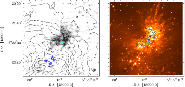
Figure 23.— Left panel: image of H i emission associated with Orion-KL, integrated over $18.7<v_{\rm LSR}<31.\;\hbox{\rm km}\;\hbox{\rm s}^{-1}$ (grayscale with white contours). Black contours indicate $1420\;\hbox{\rm MHz}$ continuum surface brightness levels of 0 to $0.5\;\hbox{\rm mJy}\;\hbox{\rm beam}^{-1}$ in steps of $0.04\;\hbox{\rm mJy}\;\hbox{\rm beam}^{-1}$. The cyan circle indicates the origin of the high velocity outflow as derived from the CO observations (Zapata et al., 2009). The dark blue stars represent the Trapezium stars. The resolution of the H i data is indicated by the ${7^{\prime\prime}\hskip-4.60007pt.\hskip 1.19995pt5}$ circular beam in the lower righthand corner of the diagram. Right panel: the same H i emission image represented by black contours, superposed on the $\hbox{\rm H}_{2}$ $v=1{-}0$ S(1) image of Bally et al. (2011). The cyan dot is as in the left panel, and the blue dot represent the position, taken from Goddi et al. (2011), of the Becklin-Neugebauer object.

6.3. High velocity H i emission from the Kleinmann-Low region

High positive velocity H i from a region approximately $45^{\prime\prime}$ in diameter (e.g., at $v_{\rm LSR}=18.7\;\hbox{\rm km}\;\hbox{\rm s}^{-1}$ in Fig. 2) extends to LSR velocities of approximately $31\;\hbox{\rm km}\;\hbox{\rm s}^{-1}$, as shown in Figs. 6 and 7. An image of this H i emission, integrated over the LSR velocity range from 18.7 to $31.0\;\hbox{\rm km}\;\hbox{\rm s}^{-1}$ is shown in Fig. 23. The high velocity H i emission coincides in position with the high velocity outflow in the Orion-KL region, embedded in the OMC-1 cloud behind the optical Huygens region.

The high velocity outflow in the Orion-KL region exhibits a wide opening angle and line-of-sight velocities of up to $100\;\hbox{\rm km}\;\hbox{\rm s}^{-1}$ in CO lines (Zuckerman et al., 1976; Kwan & Scoville, 1976). The shocked gas in this system produces luminous $\hbox{\rm H}_{2}$ vibrational line emission (Gautier et al., 1976; Nadeau & Geballe, 1979), with a spectacular morphology displaying multiple “bullets” (bow-shock tips) and “fingers” (bow-shock wakes) as shown by Allen & Burton (1993), Stolovy et al. (1998), Schultz et al. (1999), and illustrated in the $\hbox{\rm H}_{2}$ $v=1{-}0$ S(1) image shown in Fig. 23. High resolution CO observations reveal similar high velocity “bullets” and “fingers” (Chernin & Wright, 1996; Rodríguez-Franco et al., 1999b, a; Zapata et al., 2009), emerging from a common position. A number of optically identified HH objects originate from the same position (Doi et al., 2002; O’Dell & Henney, 2008; Zapata et al., 2009).

The lack of correspondence of the high velocity H i emission with prominent $\hbox{\rm H}_{2}$ and CO “fingers”, and the absence of H i emission at velocities $v_{\rm LSR}>31\;\hbox{\rm km}\;\hbox{\rm s}^{-1}$, indicates that the H i is not associated with the highest velocity outflowing gas. Nevertheless, the velocity of the observed H i with respect to OMC-1 shows that the material does participate in the outflow. The two high velocity features separated by a local minimum (Figs. 6 and 7) suggest that both outflow lobes are detected, although the northwest lobe is much more prominent in H i emission than the southeast lobe (Fig. 23). The northwest lobe displays both redshifted and blueshifted H i emission, and this situation matches that observed in CO (e.g., Chernin & Wright, 1996; Zapata et al., 2009). The southeast lobe is much less well-defined (both in H i and in CO), and it has been suggested that the outflow towards the southeast is blocked by the Orion-KL Hot Core (Chernin & Wright, 1996; Zapata et al., 2011b).

Figure 23 shows a positional match between the high velocity H i emission and the shocked $\hbox{\rm H}_{2}$ vibrational line emission, but no detailed correspondence. In fact a detailed correspondence is not expected since Fig. 23 shows only the redshifted H i, which is moving into OMC-1, away from the observer. The $\hbox{\rm H}_{2}$ emission on the other hand shows all shocked $\hbox{\rm H}_{2}$, regardless of velocity, but may be biased in favor of blueshifted gas with lower extinction. The H i is clearly concentrated in the region of the flow closest to the principal heating sources of the Orion-KL region. The lack of more extended H i emission may result from a decreasing column density as the flow expands away from its source, but may also represent photodissociation of the molecular material by UV radiation close to the heating sources.

The high velocity H i matches well, both in size and velocity, with the expanding CO shell recently discovered in Orion-KL by Zapata et al. (2011a), and centered approximately on the outflow origin. This bubble has a diameter of about $25^{\prime\prime}$, an expansion velocity of about $10\;\hbox{\rm km}\;\hbox{\rm s}^{-1}$, and a dynamical age of $500-1000\;\hbox{\rm years}$. The left panel of Fig. 23 indeed suggests that the origin of the outflow is located at a local column density minimum, bounded north, east and west by an incomplete and clumpy shell. Inspection of the CO PV diagram shown by Zapata et al. (2011a) shows that the northwest region of the CO shell is prominent in both redshifted and blueshifted emission, while in the southeast part the redshifted emission dominates, in agreement with the situation observed in H i. The precise relation of the expending CO shell to the rest of the outflow system is unknown. However, our high velocity H i data show features of both the CO shell and the inner region of the $\hbox{\rm H}_{2}$ emission, suggesting that these are directly related, and plausibly trace the same gas.

The mass in redshifted H i represented in Fig. 23 is only $2\times 10^{-5}\;\hbox{\rm M}_{\odot}$. Based on the limited velocity range sampled, the total mass of H i associated with the outflow could well be a factor of $3{-}5$ higher, i.e., $(0.6-1.0)\times 10^{-4}\;\hbox{\rm M}_{\odot}$ ($0.06-0.1$ Jupiter masses). This mass is insignificant compared to the total mass of molecular gas in the expanding bubble ($\sim 5\;\hbox{\rm M}_{\odot}$) as derived from CO (Zapata et al., 2011a).

7. H i absorption associated with the Orion Nebula

The H i absorption dataset presented in Sect. 5 shows a striking number of structures. Nevertheless, the various velocity features can be subdivided into a small number of groups, according to common properties:

1. large-scale features covering M42 as well as M43. These are the components A and B, discussed by vdWG89.

2. arclike features. These are components D and F of vdWG90 and L identified in the present dataset. in addition, component C of vdWG89 can be recognized as an extended arc;

3. elongated features displaying unique kinematic signatures. In the present data, these are components G and J.

4. features at the velocity of the background molecular cloud. These components are H, I and M.

Based on the agreement in velocity with the ionized gas, which is streaming away from OMC-1 towards us, vdWG89 interpreted component C as neutral material closely associated with the ionized gas, and suggested that this material was entrained in the ionized flow. For the blueshifted small-scale components, vdWG90 proposed acceleration by the rocket effect (Oort & Spitzer, 1955) as the origin of the blueshift with respect to the bulk of the neutral gas. For these explanations to be valid, ionization fronts would have to be present on the surfaces of the H i features. However, HST and ground-based observations have failed to reveal optical rims associated with these components (Henney et al., 2007; García-Díaz & Henney, 2007). Therefore, new interpretations for these features will be developed in the following subsections.

7.1. The large-scale atomic Veil

The large-scale structure of the atomic Veil covering M42 and M43 is dominated by H i velocity components A and B, and the red wing of the absorption lines is detected at $7.2\;\hbox{\rm km}\;\hbox{\rm s}^{-1}<v_{\rm LSR}<9.7\;\hbox{\rm km}\;\hbox{\rm s}^{-1}$ in Fig. 9. In agreement with vdWG89, a strong opacity gradient found towards the Northeast Dark Lane; a positive velocity gradient of about $2.4\;\hbox{\rm km}\;\hbox{\rm s}^{-1}\;\hbox{\rm pc}^{-1}$ is found in the same direction. This velocity gradient is detected in both components, indicating that they are related (vdWG89). vdWG89 suggested that component A represents H i in the envelope of OMC-1, extending in front of M42 and M43. A small velocity difference (H i component A is blueshifted with respect to the molecular gas by $\sim 2\;\hbox{\rm km}\;\hbox{\rm s}^{-1}$) represents a slow expansion of the cloud envelope.

7.2. Arc-like H i features

7.2.1 The southwest arc: component C

The H i absorption feature at $v_{\rm LSR}\sim-3.2\;\hbox{\rm km}\;\hbox{\rm s}^{-1}$, forming an almost semicircular arc in the southwest part of M42, is H i component C of vdWG89. The opacity images at $v_{\rm LSR}=-4.4$, $-3.2$ and $-1.9\;\hbox{\rm km}\;\hbox{\rm s}^{-1}$ show that this feature contains a string of clumps.

The system of optical flows in the southern part of M42 originates mostly from a region on the east side of the Orion-S region; Henney et al. (2007) referred to this location as the Optical Outflow Source (OOS; indicated as such in Fig. 13). Molecular outflows originate from the Orion-S cloud (summarized in Fig. 1 of O’Dell et al., 2009). Flows originating in this area branch out in multiple directions, driving several well-known HH objects (Bally et al., 2000; Henney et al., 2007). The arc formed by H i component C opens towards Orion-S. This feature may thus result from a flow originating from the Orion-S region.

A flow system located at the position angle from Orion-S towards component C was detected as an extended arc of optical emission, denoted as the Southwest Shock by Henney et al. (2007, see their Fig. 6). This feature is located approximately twice as far from the OOS as the arc formed by component C, but its shape is very similar to the H i. These features may therefore result from two separate ejections from the same object in the OOS. However, further data would be needed to verify this hypothesis.

The PV diagram shown in Fig. 15 shows the relation between component C and components A and B, that define the large-scale structure of the Veil. At small negative spatial offsets (i.e., towards the northeast), both components A and B are detected, but component C is not observed. For instance, at offset $\sim-30^{\prime\prime}$, where the lines are not saturated, both components A and B are clearly detected as kinematically separate components. This situation is different at positive offsets. Where component C appears (at offset $\sim 15^{\prime\prime}$), component B disappears. This result clearly suggests that the arc formed by component C consists of material swept up from component B, displaced towards a more negative velocity. The fact that component B is not detected in the region inside the curved arc (Fig. 14) is consistent with this interpretation.

7.2.2 The arc-like component D

Component D was first identified by vdWG90 and is the largest of the small-scale components, extending over a significant part of the Huygens region between the Trapezium stars and the Bright Bar. As noted by vdWG90, this component coincides in position and velocity with the region where velocity splitting is observed in several optical emission lines from M42. This velocity splitting was first studied in detail by Deharveng (1973), whose [N ii] $6583\;\hbox{\rm\AA}$ line-splitting region A corresponds to our H i component D. A full kinematic atlas of several optical lines has been presented by García-Díaz & Henney (2007) and García-Díaz et al. (2008); this dataset shows the line splitting in detail. The ionized gas component matching our H i component D is referred to as the “Southeast Diffuse Blue Layer” by García-Díaz & Henney (2007), who note that this component is detected in [S ii] 6716 and $6731\;\hbox{\rm\AA}$ but not in [S iii] $6312\;\hbox{\rm\AA}$. This result is important since it implies that the ionizing spectrum is rather soft, and not provided by $\theta^{1}$ C Ori. García-Díaz & Henney (2007) suggest that the blueshifted velocity component is ionized by the star $\theta^{2}$ A Ori, located southeast of the Bright Bar.

The present results shed new light on this issue. The arc-like morphology of component D was already pointed out in Sect. 5.3.2. The kinematic structure of this component suggests an expanding shell with center of expansion in the direction towards which the arc opens, i.e., southeast of the Bright Bar. Figure 13 shows that the arc opens towards the star $\theta^{2}\,$B Ori, located approximately on its axis of symmetry; this star has spectral type B0.7V (Simón-Díaz, 2010). The observed geometry suggests that this star provides the ionization for the Southeast Diffuse Blue Layer. In this model H i component D represents the neutral material outside of this H ii region. This explanation implies that an IF should be present between the Southeast Diffuse Blue Layer and H i component D; the presence of an IF is confirmed by the detection of weak [O i] $6300\;\hbox{\rm\AA}$ emission associated with this layer (García-Díaz et al., 2008).

7.2.3 The arc-like component L

The H i component L at $v_{\rm LSR}=-3.2\;\hbox{\rm km}\;\hbox{\rm s}^{-1}$ (shown by the red contours northwest of the Bright Bar in Fig. 13) displays an arc-like structure similar to that of component D, also opening towards the southeast. The characteristics of expansion are seen in Fig. 16, where it exhibits a velocity gradient with more negative velocities towards the southeast. For this component, the star $\theta^{2}\,$A Ori is located close to the symmetry axis of the arc. The spectral type of this star is O9V (Simón-Díaz et al., 2006). This configuration indicates a model identical to that described above (Sect. 7.2.2) for component D, except that here $\theta^{2}$ A Ori is the exciting star.

7.2.4 The expanding shell component F

The third component to display an expanding shell-like morphology is component F. This component is located close to a large complex of extended bow shocks in the ionized gas related to the Herbig-haro object ${\rm HH}\,{\rm 202}$. As can be seen in Fig. 13, ${\rm HH}\,{\rm 202}$ is located (in projection) at the western edge of the arc defined by H i component F. At this position, component F splits into two separate velocity components (already recognized by vdWG90 and indicated F1 and F2 in that paper). The velocity splitting is evident in Fig. 18, where component F is observed to split into two subcomponents with different spatial and kinematic offsets. The subcomponent at the most positive spatial offset matches well in position with ${\rm HH}\,{\rm 202}$.

The positions of high proper motion features in the ionized gas, shaped liked parabolic arcs, have been established by O’Dell & Henney (2008), using HST images from several epochs. The driving source for ${\rm HH}\,{\rm 202}$ is located in the OOS region associated with Orion-S (Henney et al., 2007). Indeed, a jet connecting ${\rm HH}\,{\rm 202}$ to this region has been detected in the shock-tracing [Fe ii] $1.257\;\mu\hbox{\rm m}$ line (Takami et al., 2002).

Two explanations can be considered for the presence of atomic hydrogen associated with, but not precisely superposed on ${\rm HH}\,{\rm 202}$.

1. It is possible that ${\rm HH}\,{\rm 202}$ and H i component F are formed by a jet creating a bow shock in both the ionized gas (observed as ${\rm HH}\,{\rm 202}$) and the neutral Veil (observed as H i component F), as proposed earlier by O’Dell et al. (1997).

2. Alternatively, it is possible that H i component F results from rapid recombination in the dense post-shock gas associated with ${\rm HH}\,{\rm 202}$. This model has been proposed by Mesa-Delgado et al. (2009), who show that in ${\rm HH}\,{\rm 202{-}S}$ (the brightest knot in ${\rm HH}\,{\rm 202}$) the post-shock density is sufficiently high to trap the IF. As a result, the gas behind this dense post-shock region is shielded from the ionizing radition of the Trapezium stars, and rapidly recombines and cools.

3. Finally, it is possible for this component that the acceleration is provided by the rockets effect described by Oort & Spitzer (1955).

In the second and third models, the neutral H i should be located behind the IF in the direction away from the Trapezium stars, i.e., west of the bright rims of ${\rm HH}\,{\rm 202}$. However, none of the absorbing H i is located in this region, and most of it is in fact located east of ${\rm HH}\,{\rm 202}$. This geometry argues against the last two models. In addition, a strong argument in favour of the first of these three models comes from the fact that the blueshifted H i gas forming component F corresponds to a gap in the Veil, as observed in Fig. 18. This is exactly the geometry that is expected when part of the Veil gas is accelerated to a more negative velocity by the impact of a jet. In summary, the location of the H i with respect to ${\rm HH}\,{\rm 202}$, and its detailed kinematic structure argue in favour of an interaction of the jet driving ${\rm HH}\,{\rm 202}$ with the neutral Veil.

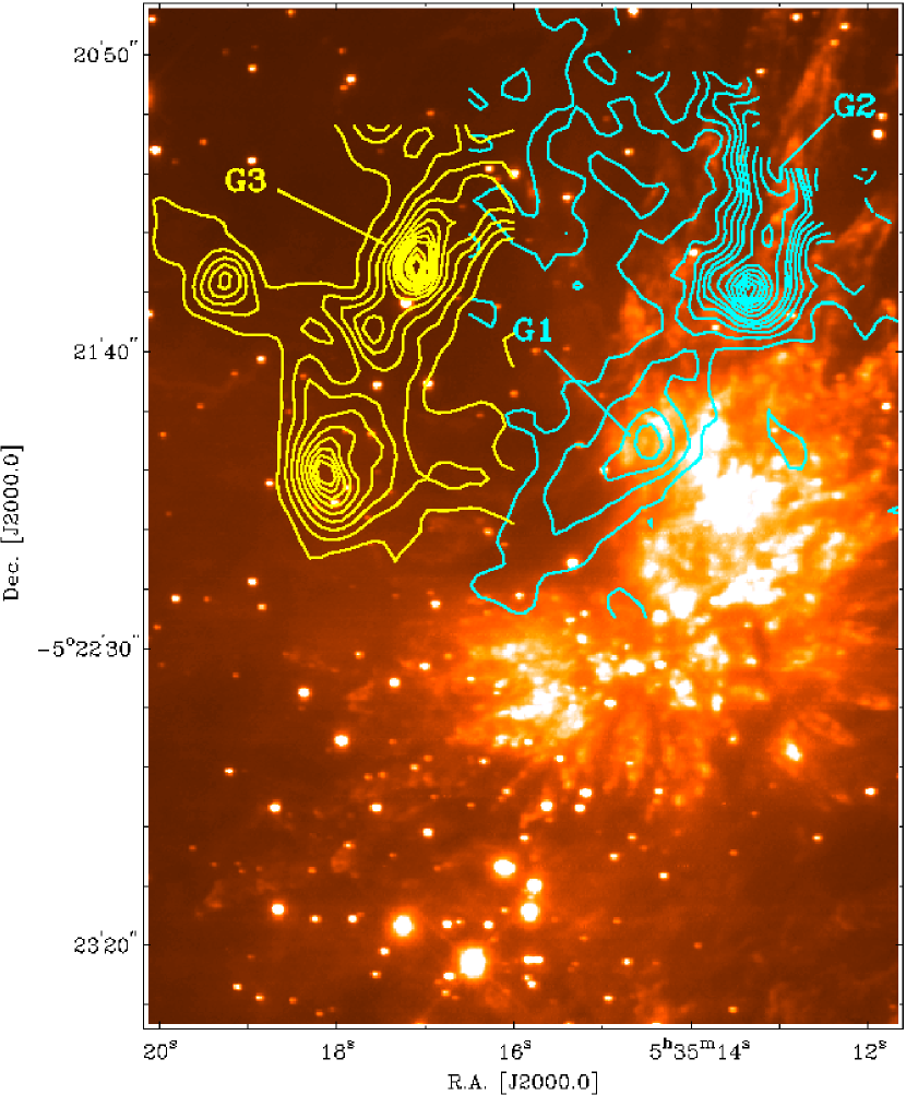
Figure 24.— H i opacity contours overlayed on the $\hbox{\rm H}_{2}$ $v=1{-}0$ S(1) image of Bally et al. (2011). Light blue contours show H i opacity at $v_{\rm LSR}=-9.6\;\hbox{\rm km}\;\hbox{\rm s}^{-1}$ from H i components G1 and G2, with contour levels from 0.1 to 0.6 in steps of 0.1, then from 0.8 to 1.8 in steps of 0.2. Yellow contours show H i opacity at $v_{\rm LSR}=-0.6\;\hbox{\rm km}\;\hbox{\rm s}^{-1}$ from component G3, with contour levels from 0.50 to 2.25 in steps of 0.25, then from 2.5 to 4.0 in steps of 0.5.

7.3. Elongated H i features

Among the kinematic H i features identified, components G and J have an obvious elongated appearance, quite distinct from the arc-like features discussed above.

7.3.1 Component G

The Northern part of M42, where component G is located, harbors a system of optical HH objects (e.g., ${\rm HH}\,{\rm 201}$, ${\rm HH}\,{\rm 205{-}210}$, all indicated in Fig. 13), which are associated with the complex and spectacular system of “fingers” observed in $\hbox{\rm H}_{2}$ vibrational line emission (Allen & Burton, 1993; Salas et al., 1999; Bally et al., 2011) and CO (Zapata et al., 2009). Emission in the shock tracing [Fe ii] $1.64\;\mu\hbox{\rm m}$ line is found at the tips of the fingers. The fact that these “fingers” display optical line emission shows that in this region they have broken out of the background molecular cloud towards us (O’Dell et al., 1997).

In the present H i data, several velocity systems are found in this region, as can be seen in Fig. 20. The highest (negative) velocities are found for component G2 (light blue contours in Fig. 13), and this component is, in location as well as orientation, closely aligned with the line connecting the “dynamical center” where this outflow system originates (as discussed in Sect. 6.3) to the Herbig-Haro objects ${\rm HH}\,{\rm 205{-}207}$. This line also corresponds to one of the most prominent molecular “fingers”: the 1:00 system in the (hour dial) notation of O’Dell et al. (1997). This agreement is shown in Fig. 24, where component G2 is shown in the blue contours at Declination north of $-5^{\circ}\,21^{\prime}\,40^{\prime\prime}$. South of this Declination, the blue contours trace component G1, and Fig. 24 shows that this feature does not correspond to any of the shocked $\hbox{\rm H}_{2}$ features and, given its orientation, does not originate in the Orion-KL region. At less negative velocities, component G3, which is approximately aligned with G1 but displaced eastwards, is prominent, as shown in Fig. 24 by the yellow contours. If components G1 and G3 originate from a common source, this source must be located approximately $30^{\prime\prime}$ east of the Trapezium stars. However, this region does not harbour any known driving source for these flows.

The asssociation of component G2 with the $\hbox{\rm H}_{2}$ “finger” system related to the Orion-KL outflow enables a new estimate of the line-of-sight location of the dynamical center of the outflow behind the IF. The Herbig-Haro object ${\rm HH}\,{\rm 205}$ is associated with this $\hbox{\rm H}_{2}$ “finger”, and closely aligned with H i component G2 (Fig. 13). The radial velocity of ${\rm HH}\,{\rm 205}$ is $v_{\rm LSR}=-200\;\hbox{\rm km}\;\hbox{\rm s}^{-1}$ (O’Dell et al., 1997), while its tangential velocity has been measured to be $320\;\hbox{\rm km}\;\hbox{\rm s}^{-1}$ (Bally et al., 2000). This system thus follows a trajectory with an angle of $\sim 30^{\circ}\hskip-2.84544pt$ relative to the plane of the sky. The position where the $\hbox{\rm H}_{2}$ “finger” breaks through the IF is displaced from the dynamical center of the outflow by a projected distance of $0.14\;\hbox{\rm pc}$. Combining these results yields a distance of the dynamical center of the outflow of $\sim 0.1\;\hbox{\rm pc}$ behind the IF. This distance is somewhat smaller than the $\sim 0.2\;\hbox{\rm pc}$ derived by Doi et al. (2004) using a similar calculation based on the velocity vector and location of the Herbig-Haro object ${\rm HH}\,{\rm 201}$ (Graham et al., 2003).

7.3.2 Components J and K

The other elongated H i feature in our dataset is component J, which crosses the Bright Bar orthogonally. This feature is best seen at $v_{\rm LSR}=-3.2\;\hbox{\rm km}\;\hbox{\rm s}^{-1}$ in Fig. 9. Both in position and orientation, this feature closely coincides with the large, bright pair ${\rm HH}\,{\rm 203{/}204}$. Inspection of the H i opacity images in Fig. 9 shows a peak in H i opacity located at the position of ${\rm HH}\,{\rm 203}$ at LSR velocities from $-7.0$ to $-4.3\;\hbox{\rm km}\;\hbox{\rm s}^{-1}$. However, at $-3.2\;\hbox{\rm km}\;\hbox{\rm s}^{-1}$ an extension towards ${\rm HH}\,{\rm 204}$ is apparent, so that H i is associated with both Herbig-Haro objects. O’Dell et al. (1997) suggested that these objects mark the points where collimated flows impact the extended H i Veil. The detection of H i associated with these features provides support for this model.

H i component K, located south of J, coincides with a region resembling a bow shock (see Fig. 6 of Henney et al., 2007). This region displays high ionization emission ([O iii]) as well as prominent lower ionization ([N ii] and [S ii]) ridges. This region may represent an outer shock related to the ${\rm HH}\,{\rm 203{/}204}$ system and would again be the result of a collimated flow striking the Veil.

7.4. The blueshifted H i feature E

The remaining blueshifted H i feature, component E, appears neither arc-like nor elongated and thus does not fit into any of the above categories.

Component E is located in the region of the Dark Bay. This feature consists of 10 unresolved or barely resolved clumps, forming a coherent velocity structure (Fig. 17). Due to the lack of detailed optical information in the Dark Bay region, no associations with ionized gas flows can be established. However, the different morphology of component E as well as the larger linewidth compared to the other H i components suggests that component E does not arise from the same process. As noted in Sect. 6.2, the Dark Bay gas is at $v_{\rm LSR}\approx 6\;\hbox{\rm km}\;\hbox{\rm s}^{-1}$. Component E is therefore signficantly blueshifted with respect to the bulk of the Dark Bay gas. An attractive hypothesis is that H i component E arises in a PDR related to the Dark Bay, at the side facing the ONC. The thermal expansion of the H ii region may then account for the blueshift of H i absorption with respect to rest of the Dark Bay gas.

7.5. H i features at the velocity of the background molecular cloud

H i components H, I and M have central velocities $v_{\rm LSR}=9-10\;\hbox{\rm km}\;\hbox{\rm s}^{-1}$, corresponding to the velocity of OMC-1. Since these features are observed in absorption, a significant radio continuum must arise behind them. Component I has already been discussed above (Sect. 6.2), in connection with the H i emission associated with that component.

7.5.1 Component H: H i absorption from Orion-S

The H i absorption component H (which was already noted by vdWG90) corresponds closely in location, velocity, extent and morphology with an $\hbox{\rm H}_{2}\hbox{\rm CO}$ absorption feature first identified by Johnston et al. (1983) and studied at higher resolution by Mangum et al. (1993), as indicated in Fig. 13. This feature is related to the Orion-S molecular core. The detection of Orion-S in absorption indicates that the IF separating M42 from OMC-1 must be located behind Orion-S. The implication is that the Orion-S molecular core must be located within the ionized nebula. O’Dell et al. (2009) were the first to argue for this geometry, based on the detection of $\hbox{\rm H}_{2}\hbox{\rm CO}$ absorption and anomalies in the derived extinction; the present H i data confirm this picture. The detailed 3-dimensional structure and the physical association of the various features in this region are discussed in detail by O’Dell et al. (2009). These authors also construct a physical model of the region, showing that the density and column density are sufficient for Orion-S to survive in the harsh radiation environment of M42.

7.5.2 H i absorption associated with the Bright Bar

H i produced in the Orion Bar PDR will be at $v_{\rm LSR}=10\;\hbox{\rm km}\;\hbox{\rm s}^{-1}$, as derived from molecular lines in this region (e.g., Fig. 8 of Van der Werf et al., 1996). The collection of clumps which we have collectively labeled component M (as indicated in the opacity image at $11.1\;\hbox{\rm km}\;\hbox{\rm s}^{-1}$ in Fig. 9), closely trace the outside of the Bright Bar and most likely represent clumps of photodissociated H i in the Orion Bar PDR. The small but non-zero angle of the IF with respect to edge-on causes most of the photodissociated gas to be located behind the radio continuum of the Bar; this H i cannot be dectected in absorption. However, since the IF will not be flat, a background radio continuum will be available over a small distance towards the southeast in regions where small amounts of H i are located in concave sections of the IF. Towards this continuum the H i can be observed in absorption. At larger distances from the IF, photodissociated H i in the Orion Bar PDR is observed in emission, as discussed in Sect. 6.1.

7.6. Non-detection of H i from proplyds

No H i absorption was found associated with known proplyds in the Orion Nebula, with upper limits of about a Jupiter mass. This result indicates that evaporation and ablation of molecular gas associated with the proplyds (Chen et al., 1998; Henney & O’Dell, 1999; Henney et al., 2002) is rapidly followed by photoionization. Alternatively, the external IF confining the proplyds may be opaque in the $21\;\hbox{\rm cm}$ continuum, prohibiting the detection of neutral hydrogen.

8. The Veil of Orion

8.1. Location of the Veil

Several of the blueshifted velocity components show clear evidence of interaction with the Veil. This behavior is most obvious for component F, where the Veil shows a gap corresponding closely in position with the blueshifted gas of component F (Sect. 5.3.4). Similar evidence is found for component C (Sect. 7.2.1). For component G the evidence for interaction with the Veil is weaker, but it clearly reveals interaction with a layer of neutral gas.

Component F therefore plays a crucial role in analysis of the interaction of the ionized flows with the Veil. This component is driven by the prominent HH object ${\rm HH}\,{\rm 202}$, for which the space velocity vector is known, since both radial and tangential velocities have been determined (Doi et al., 2002, 2004; Henney et al., 2007; O’Dell & Henney, 2008). This flow system originates in the OOS associated with Orion-S; therefore its radial distance with respect to Orion-S can be calculated. This distance is found to be $0.17\;\hbox{\rm pc}$ (Doi et al., 2004). The lateral extent of the ${\rm HH}\,{\rm 202}$-component F system is about $50^{\prime\prime}$ or $0.11\;\hbox{\rm pc}$, and this size can be used as the maximum distance between ${\rm HH}\,{\rm 202}$ and H i component F. We conclude that H i component F, and therefore the neutral Veil, is located at most $0.3\;\hbox{\rm pc}$ in front of Orion S.

This distance is to be compared to the $\sim 1\;\hbox{\rm pc}$ distance between the Trapezium stars and the Veil, estimated by Abel et al. (2004). The relative line-of-sight distances of Orion-S and the Trapezium stars are unknown. O’Dell et al. (2009) argue that Orion-S cannot be much behind the Trapezium stars, or else it would not be possible to distinguish it from main IF separating M42 from OMC-1. On the other hand, if Orion-S were significantly in front of the Trapezium stars, it would be in front of almost all optical line emission, and create a conspicuous extinction feature. While an extinction feature at this position has indeed been detected, it is not very prominent (O’Dell & Yusef-Zadeh, 2000), and significantly less pronounced than for instance the Dark Bay, which is indeed located in front of the ionized nebula. Considering the large column density of Orion-S, its relatively modest derived extinction must be due to the fact that a significant fraction of the nebular emission arises in front of it. Therefore Orion-S is unlikely to be much closer to the Veil than the Trapezium stars.

An additional argument can be found in the morphology of H i component H, which corresponds to Orion-S. The absorbing H i displays an opacity peak at its north edge, i.e., approximately facing the Trapezium stars. At the same position a small local maximum in radio continuum is found. This geometry suggests that the ionizing and dissociating radiation has created an IF and PDR at the side of Orion-S facing the Trapezium. The implication is that this radiation must come mostly from the side, and that the line of sight connecting Orion-S and the Trapezium stars is unlikely to be inclined more than $45^{\circ}\hskip-2.84544pt$ from the plane of the sky. This argument suggests that Orion-S is unlikely to lie more than $0.1\;\hbox{\rm pc}$ in front of the Trapezium stars. The surface of the Veil facing the ionized nebula will then be at most $0.4\;\hbox{\rm pc}$ in front of the Trapezium stars.

Observations of UV absorption lines reveal local densities in the Veil, also providing limits on the distance of the Veil from the Trapezium stars (Abel et al., 2004, 2006). An upper distance limit of $3\;\hbox{\rm pc}$ was determined by the absence of strong $\hbox{\rm H}_{2}$ UV absorption lines, which implies a significant UV field to keep the molecular hydrogen fraction at the observed value. A lower limit to the distance of the Veil to the Trapezium stars was provided by Abel et al. (2004). These authors show the detailed dependence of a large number of observables on the Veil-Trapezium distance. In addition they used limits on $\hbox{{\rm H}}\beta$ and [N ii] $6583\;\hbox{\rm\AA}$ emission from the surface of the Veil facing the Trapezium to derive a minimum Veil-Trapezium distance of $0.33\;\hbox{\rm pc}$ (for $\hbox{{\rm H}}\beta$) and $1\;\hbox{\rm pc}$ (for [N ii]). The [N ii] emission was however considered in more detail by Abel et al. (2006), who demonstrated the presence of a density-bounded layer of ionized gas located between the Trapezium and the Veil and moving towards the Veil. These authors conclude that this layer absorbs most of the ionizing radiation from the Trapezium stars, which accounts for the absence of a pronounced IF at the surface of the Veil facing the Trapezium. This result has the important implication that the emission line surface brightness of the illuminated side of the Veil cannot be used to constrain its distance to the Trapezium. In summary, we conclude that the distance between the Veil and the Trapezium of $0.4\;\hbox{\rm pc}$ derived in this paper is consistent with the analysis by Abel et al. (2004) and Abel et al. (2006).

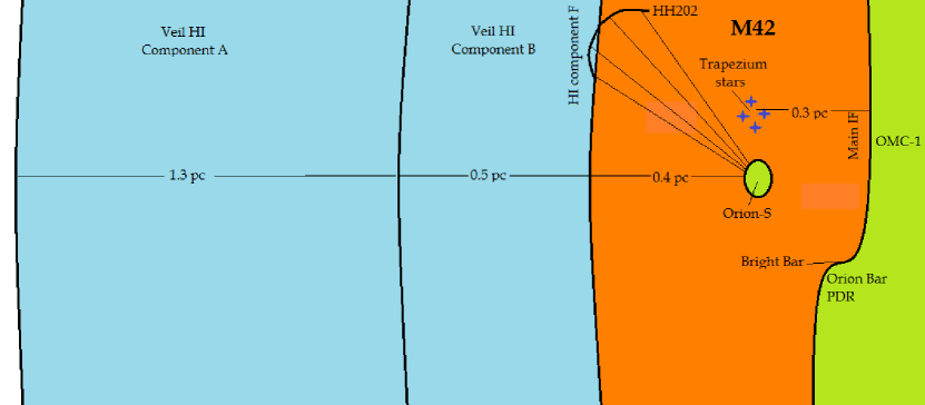
Figure 25.— Schematic geometry of M42 and the neutral Veil, illustrating the line-of-sight depths (approximately but not exactly to scale) of the various components. Orange indicates ionized gas, green indicates molecular gas and blue indicates atomic gas. The outflow originating in Orion-S, which powers the kinematics of ${\rm HH}\,{\rm 202}$ and H i component F is schematically indicated by a set of thin lines.

8.2. Geometry of the Orion Nebula and the Veil

Our results reveal direct interaction of ionizing flows originating close to Orion-S with the Veil. The evidence is particularly strong for the ${\rm HH}\,{\rm 202}$ (H i component F, Sect. 7.2.4), which shows that only velocity component B of the Veil is affected. This result implies that component B is located closer to the ionized gas than component A, and for the first time reveals the relative locations of the two velocity components that constitute the Veil. As noted in Sect. 7.1, these two H i components are large-scale features covering both M42 and M43, and exhibiting a common velocity gradient, indicating that they are related. The fact that they both display a high and similar line-of-sight magnetic field strength (Troland et al., 1989) reinforces this conclusion. As shown by Abel et al. (2004), the magnetic energy exceeds the energy in turbulent motions at least in component A, where it constitutes the dominant pressure term. Ferland (2009) has suggested that this situation is the result of compression by the expanding H ii region and radiation pressure from the ONC.

The H i column densities in components A and B, based on $\hbox{{\rm Ly}}\alpha$ absorption measurements, are approximately 1.6 and $3.2\cdot 10^{21}\;\hbox{\rm cm}^{-2}$ respectively (Abel et al., 2006). With the best density estimates of approximately $10^{2.5}$ and $10^{3.4}\;\hbox{\rm cm}^{-3}$ for A and B (Abel et al., 2006), their thicknesses are approximately 1.3 (A) and $0.5\;\hbox{\rm pc}$ (B). The resulting geometry is schematically shown in Fig. 25. The lateral extent of the Veil is at least $1.5\;\hbox{\rm pc}$ (its total extent covering M42 and M43), but probably significantly larger, since it represents the atomic envelope of the background molecular cloud (vdWG89), which extends over at least $10\;\hbox{\rm pc}$, approximately the length of integral-shaped filament of molecular gas and dust Bally et al. (1987); Johnstone & Bally (1999). The total depth of the ionized cavity is about $0.7\;\hbox{\rm pc}$, which is small compared both to the lateral extent of the Veil and to its depth of approximately $1.8\;\hbox{\rm pc}$. These results therefore demonstrate the blister-type nature of the M42 H ii region, emphasized by main IF behind the Trapezium stars, and also reveal its relation to the envelope of the background molecular cloud, represented by the Veil.

9. Conclusions

High resolution H i observations of the Orion Nebula reveal in detail the feedback of the H ii region and the ONC on their neutral environment. This feedback takes place through both radiative and mechanical interaction. Furthermore, our data provide new information on the geometry of the complex.

Radiative feedback manifests itself principally by the non-ionizing UV radiation from the ONC, which creates a prominent PDR outside the IF at the interface between M42 and OMC-1. Prominent H i emission is detected from the Orion Bar PDR, southeast of the Bright Bar IF. This result enables for the first time a study of the abundance profile of atomic hydrogen and its relation to other tracers in an edge-on PDR. We find that the H i emission arises from a region with a temperature of $\sim 540\;\hbox{\rm K}$, with $\approx 5-10\%$ of the hydrogen nuclei in the interclump region in the PDR in the form of H i. Most of the hydrogen in the region probed therefore remains molecular, in agreement with theoretical PDR models. This result shows that dense PDRs such as the Orion Bar PDR have a low H i production, even if the impinging UV radiation field is very strong. The H i column density peak matches the peak of UV-excited vibrational $\hbox{\rm H}_{2}$ line emission. This result confirms the two-step $\hbox{\rm H}_{2}$ photodissociation process through UV line absorption in the Lyman and Werner bands.

Mechanical feedback results from the interaction of ionized and molecular outflow systems with the neutral environment of the H ii region. The H i data provides direct evidence for interaction of the HH object ${\rm HH}\,{\rm 202}$ and the flow system responsible for the optical Southwest Shock of Henney et al. (2007) with the Veil. The interaction of these flow systems with the Veil causes velocity shifts in the absorbing H i. The evidence for direct interaction between ${\rm HH}\,{\rm 202}$ and the neutral Veil implies that the Veil must be located quite close to the Orion-S source of outflows. Using the known space trajectory of ${\rm HH}\,{\rm 202}$, we find that the surface of Veil facing the Orion Nebula is located at most $0.4\;\hbox{\rm pc}$ in front of Orion-S. Of the two velocity components A and B that constitute the Veil, we find that component B lies closer to the ionized nebula.

The total depth of the ionized cavity is approximately $0.7\;\hbox{\rm pc}$. This depth is small compared to both the lateral extent and the depth of Veil. These dimensions confirm the nature of the M42 H ii region as a thin blister, and simultaneously reveal the relation of the ionized region to the background molecular cloud and its neutral envelope.

Appendix A Relation between H i column density and 21 cm line optical depth and brightness temperature

The H i column density is related to the velocity-integrated optical depth of the $21\;\hbox{\rm cm}$ line by

$$N(\hbox{{\rm H}}\,\hbox{{\sc i}})={32\pi kT_{\rm s}\over 3A_{\rm ul}hc\lambda_{\rm ul}^{2}}\int\tau(v)\,dv,$$ (A1)

where $\lambda_{\rm ul}=21.10612\;\hbox{\rm cm}$ is the wavelength of the transition, $A_{\rm ul}=2.88426\cdot 10^{-15}\;\hbox{\rm s}^{-1}$ (Gould, 1994) is its Einstein $A$ value, $T_{\rm s}$ is the spin temperature (i.e., the excitation temperature of the two spin levels), $h$ is Planck’s constant, $k$ is the Boltzmann constant, and $c$ is the speed of light. This expression makes use of the approximation $\exp(-E_{\rm ul}/kT_{\rm s})\approx 1-E_{\rm ul}/kT_{\rm s}$, where $E_{\rm ul}$ is the energy difference of the two spin levels. This approximation is valid to high accuracy, since $E_{\rm ul}/k=0.06816\;\hbox{\rm K}$ and $T_{\rm s}\gg E_{\rm ul}/k$ under all practical conditions. Inserting numbers, Eq. $\left(\ref{eq.NHI}\right)$ can be written as

$${N(\hbox{{\rm H}}\,\hbox{{\sc i}})\over{\rm cm}^{-2}}=1.81267\cdot 10^{18}\,{T_{\rm s}\over{\rm K}}\int\tau(v)\,d{v\over{\rm km}\;\hbox{\rm s}^{-1}}.$$ (A2)

For optically thin ($\tau(v)\ll 1$) H i emission, $\exp{[-\tau(v)]}$ can be expanded to first order and the equation of transfer Eq. $\left(\ref{eq.Transfer}\right)$ reduces to

$$T_{\rm b}(v)=\tau(v)[T_{\rm s}-T_{\rm c}-T_{\rm back}(v)].$$ (A3)

If $T_{\rm s}\gg T_{\rm c}+T_{\rm back}(v)$ in Eq. $\left(\ref{eq.TransferThin}\right)$, the H i column density as given by Eq. $\left(\ref{eq.NHI}\right)$ can be expressed as

$$N(\hbox{{\rm H}}\,\hbox{{\sc i}})={32\pi kT_{\rm s}\over 3A_{\rm ul}hc\lambda_{\rm ul}^{2}}\int T_{\rm b}(v)\,dv,$$ (A4)

which results in

$${N(\hbox{{\rm H}}\,\hbox{{\sc i}})\over{\rm cm}^{-2}}=1.81267\cdot 10^{18}\,{\int T_{\rm b}(v)\,dv\over{\rm K}\;\hbox{\rm km}\;\hbox{\rm s}^{-1}}.$$ (A5)

References

- Abel et al. (2004) Abel, N. P., Brogan, C. L., Ferland, G. J., O’Dell, C. R., Shaw, G., & Troland, T. H. 2004, ApJ, 609, 247
- Abel et al. (2006) Abel, N. P., Ferland, G. J., O’Dell, C. R., Shaw, G., & Troland, T. H. 2006, ApJ, 644, 344
- Allen & Burton (1993) Allen, D. A., & Burton, M. G. 1993, Nature, 363, 54
- Allers et al. (2005) Allers, K. N., Jaffe, D. T., Lacy, J. H., Draine, B. T., & Richter, M. J. 2005, ApJ, 630, 368
- Ascasibar et al. (2011) Ascasibar, Y., Obreja, A. C., & Díaz, A. I. 2011, MNRAS, 1070
- Balick et al. (1974) Balick, B., Gammon, R. H., & Hjellming, R. M. 1974, PASP, 86, 616
- Bally (2008) Bally, J. 2008, in Handbook of Star Forming Regions, Volume I, ed. Reipurth, B. (ASP), 459–+
- Bally et al. (2011) Bally, J., Cunningham, N. J., Moeckel, N., Burton, M. G., Smith, N., Frank, A., & Nordlund, A. 2011, ApJ, 727, 113
- Bally et al. (1987) Bally, J., Langer, W. D., Stark, A. A., & Wilson, R. W. 1987, ApJ, 312, L45
- Bally et al. (2000) Bally, J., O’Dell, C. R., & McCaughrean, M. J. 2000, AJ, 119, 2919
- Blaauw (1964) Blaauw, A. 1964, ARA&A, 2, 213
- Black & Van Dishoeck (1987) Black, J. H., & Van Dishoeck, E. F. 1987, ApJ, 322, 412
- Blouin et al. (1997) Blouin, D., McCutcheon, W. H., Dewdney, P. E., Roger, R. S., Purton, C. R., Kester, D., & Bontekoe, T. R. 1997, MNRAS, 287, 455
- Boisse (1990) Boisse, P. 1990, A&A, 228, 483
- Bregman et al. (1994) Bregman, J., Larson, K., Rank, D., & Temi, P. 1994, ApJ, 423, 326
- Buckle et al. (2012) Buckle, J. V., et al. 2012, MNRAS, 422, 521
- Burton et al. (1990) Burton, M. G., Hollenbach, D. J., & Tielens, A. G. G. M. 1990, ApJ, 365, 620
- Castets et al. (1990) Castets, A., Duvert, G., Dutrey, A., Bally, J., Langer, W. D., & Wilson, R. W. 1990, A&A, 234, 469
- Chen et al. (1998) Chen, H., Bally, J., O’dell, C. R., McCaughrean, M. J., Thompson, R. L., Rieke, M., Schneider, G., & Young, E. T. 1998, ApJ, 492, L173
- Chernin & Wright (1996) Chernin, L. M., & Wright, M. C. H. 1996, ApJ, 467, 676
- Chromey et al. (1989) Chromey, F. R., Elmegreen, B. G., & Elmegreen, D. M. 1989, AJ, 98, 2203
- Clark (1965) Clark, B. G. 1965, ApJ, 142, 1398
- Clark et al. (1962) Clark, B. G., Radhakrishnan, V., & Wilson, R. W. 1962, ApJ, 135, 151
- Deharveng (1973) Deharveng, L. 1973, A&A, 29, 341
- Dewdney & Roger (1982) Dewdney, P. E., & Roger, R. S. 1982, ApJ, 255, 564
- Dewdney & Roger (1986) —. 1986, ApJ, 307, 275
- Doi et al. (2002) Doi, T., O’Dell, C. R., & Hartigan, P. 2002, AJ, 124, 445
- Doi et al. (2004) —. 2004, AJ, 127, 3456
- Draine (1978) Draine, B. T. 1978, ApJS, 36, 595
- Draine & Bertoldi (1996) Draine, B. T., & Bertoldi, F. 1996, ApJ, 468, 269
- Ferland (2009) Ferland, G. J. 2009, in IAU Symposium, Vol. 259, IAU Symposium, 25–34
- Field et al. (1966) Field, G. B., Somerville, W. B., & Dressler, K. 1966, ARA&A, 4, 207
- García-Díaz & Henney (2007) García-Díaz, M. T., & Henney, W. J. 2007, AJ, 133, 952
- García-Díaz et al. (2008) García-Díaz, M. T., Henney, W. J., López, J. A., & Doi, T. 2008, Rev. Mex. Astron. Astr., 44, 181
- Gautier et al. (1976) Gautier, III, T. N., Fink, U., Larson, H. P., & Treffers, R. R. 1976, ApJ, 207, L129
- Genzel et al. (1981) Genzel, R., Reid, M. J., Moran, J. M., & Downes, D. 1981, ApJ, 244, 884
- Genzel & Stutzki (1989) Genzel, R., & Stutzki, J. 1989, ARA&A, 27, 41
- Gezari et al. (1998) Gezari, D. Y., Backman, D. E., & Werner, M. W. 1998, ApJ, 509, 283
- Goddi et al. (2011) Goddi, C., Humphreys, E. M. L., Greenhill, L. J., Chandler, C. J., & Matthews, L. D. 2011, ApJ, 728, 15
- Goss & Shaver (1970) Goss, W. M., & Shaver, P. A. 1970, Australian Journal of Physics Astrophysical Supplement, 14, 1
- Gould (1994) Gould, R. J. 1994, ApJ, 423, 522
- Graham et al. (2003) Graham, M. F., Meaburn, J., & Redman, M. P. 2003, MNRAS, 343, 419
- Green (1991) Green, D. A. 1991, MNRAS, 253, 350
- Güdel et al. (2008) Güdel, M., Briggs, K. R., Montmerle, T., Audard, M., Rebull, L., & Skinner, S. L. 2008, Science, 319, 309
- Hayashi et al. (1985) Hayashi, M., Hasegawa, T., Gatley, I., Garden, R., & Kaifu, N. 1985, MNRAS, 215, 31P
- Henney & O’Dell (1999) Henney, W. J., & O’Dell, C. R. 1999, AJ, 118, 2350
- Henney et al. (2002) Henney, W. J., O’Dell, C. R., Meaburn, J., Garrington, S. T., & Lopez, J. A. 2002, ApJ, 566, 315
- Henney et al. (2007) Henney, W. J., O’Dell, C. R., Zapata, L. A., García-Díaz, M. T., Rodríguez, L. F., & Robberto, M. 2007, AJ, 133, 2192
- Herrmann et al. (1997) Herrmann, F., Madden, S. C., Nikola, T., Poglitsch, A., Timmermann, R., Geis, N., Townes, C. H., & Stacey, G. J. 1997, ApJ, 481, 343
- Heyer et al. (1992) Heyer, M. H., Morgan, J., Schloerb, F. P., Snell, R. L., & Goldsmith, P. F. 1992, ApJ, 395, L99
- Hillenbrand & Hartmann (1998) Hillenbrand, L. A., & Hartmann, L. W. 1998, ApJ, 492, 540
- Hirota et al. (2007) Hirota, T., et al. 2007, PASJ, 59, 897
- Hogerheijde et al. (1995) Hogerheijde, M. R., Jansen, D. J., & van Dishoeck, E. F. 1995, A&A, 294, 792
- Hollenbach & Tielens (1999) Hollenbach, D. J., & Tielens, A. G. G. M. 1999, Reviews of Modern Physics, 71, 173
- Huygens (1659) Huygens, C. 1659, Systema Satvrnivm (The Hague: A. Vlacq)
- Jaffe & Pankonin (1978) Jaffe, D. T., & Pankonin, V. 1978, ApJ, 226, 869
- Jansen et al. (1995) Jansen, D. J., Spaans, M., Hogerheijde, M. R., & van Dishoeck, E. F. 1995, A&A, 303, 541
- Johnston et al. (1983) Johnston, K. J., Palmer, P., Wilson, T. L., & Bieging, J. H. 1983, ApJ, 271, L89
- Johnstone & Bally (1999) Johnstone, D., & Bally, J. 1999, ApJ, 510, L49
- Johnstone et al. (2003) Johnstone, D., Boonman, A. M. S., & van Dishoeck, E. F. 2003, A&A, 412, 157
- Joncas et al. (1992) Joncas, G., Durand, D., & Roger, R. S. 1992, ApJ, 387, 591
- Kaler (1967) Kaler, J. B. 1967, ApJ, 148, 925
- Kassis et al. (2006) Kassis, M., Adams, J. D., Campbell, M. F., Deutsch, L. K., Hora, J. L., Jackson, J. M., & Tollestrup, E. V. 2006, ApJ, 637, 823
- Kaufman et al. (1999) Kaufman, M. J., Wolfire, M. G., Hollenbach, D. J., & Luhman, M. L. 1999, ApJ, 527, 795
- Kleinmann & Low (1967) Kleinmann, D. E., & Low, F. J. 1967, ApJ, 149, L1+
- Kraus et al. (2007) Kraus, S., et al. 2007, A&A, 466, 649
- Kutner et al. (1977) Kutner, M. L., Tucker, K. D., Chin, G., & Thaddeus, P. 1977, ApJ, 215, 521
- Kwan & Scoville (1976) Kwan, J., & Scoville, N. 1976, ApJ, 210, L39
- Le Petit et al. (2006) Le Petit, F., Nehmé, C., Le Bourlot, J., & Roueff, E. 2006, ApJS, 164, 506
- Lis & Schilke (2003) Lis, D. C., & Schilke, P. 2003, ApJ, 597, L145
- Lockhart & Goss (1978) Lockhart, I. A., & Goss, W. M. 1978, A&A, 67, 355
- Loren (1979) Loren, R. B. 1979, ApJ, 234, L207
- Luhman et al. (1998) Luhman, K. L., Engelbracht, C. W., & Luhman, M. L. 1998, ApJ, 499, 799
- Lykins et al. (2010) Lykins, M. L., Abel, N., & Troland, T. H. 2010, ApJ, 713, 950
- Maddalena et al. (1986) Maddalena, R. J., Morris, M., Moscowitz, J., & Thaddeus, P. 1986, ApJ, 303, 375
- Mangum et al. (1993) Mangum, J. G., Wootten, A., & Plambeck, R. L. 1993, ApJ, 409, 282
- Marconi et al. (1998) Marconi, A., Testi, L., Natta, A., & Walmsley, C. M. 1998, A&A, 330, 696
- Martins et al. (2005) Martins, F., Schaerer, D., & Hillier, D. J. 2005, A&A, 436, 1049
- Meijerink et al. (2007) Meijerink, R., Spaans, M., & Israel, F. P. 2007, A&A, 461, 793
- Meixner & Tielens (1993) Meixner, M., & Tielens, A. G. G. M. 1993, ApJ, 405, 216
- Menten et al. (2007) Menten, K. M., Reid, M. J., Forbrich, J., & Brunthaler, A. 2007, A&A, 474, 515
- Mesa-Delgado et al. (2009) Mesa-Delgado, A., Esteban, C., García-Rojas, J., Luridiana, V., Bautista, M., Rodríguez, M., López-Martín, L., & Peimbert, M. 2009, MNRAS, 395, 855
- Mezger et al. (1990) Mezger, P. G., Zylka, R., & Wink, J. E. 1990, A&A, 228, 95
- Mills & Shaver (1968) Mills, B. Y., & Shaver, P. A. 1968, Australian Journal of Physics, 21, 95
- Muench et al. (2008) Muench, A., Getman, K., Hillenbrand, L., & Preibisch, T. 2008, in Handbook of Star Forming Regions, Volume I, ed. Reipurth, B. (ASP), 483–+
- Muller (1959) Muller, C. A. 1959, in IAU Symposium, Vol. 9, URSI Symp. 1: Paris Symposium on Radio Astronomy, ed. R. N. Bracewell, 360
- Nadeau & Geballe (1979) Nadeau, D., & Geballe, T. R. 1979, ApJ, 230, L169
- Natta et al. (1994) Natta, A., Walmsley, C. M., & Tielens, A. G. G. M. 1994, ApJ, 428, 209
- O’Dell (2001) O’Dell, C. R. 2001, ARA&A, 39, 99
- O’Dell & Harris (2010) O’Dell, C. R., & Harris, J. A. 2010, AJ, 140, 985
- O’Dell et al. (1997) O’Dell, C. R., Hartigan, P., Lane, W. M., Wong, S. K., Burton, M. G., Raymond, J., & Axon, D. J. 1997, AJ, 114, 730
- O’Dell & Henney (2008) O’Dell, C. R., & Henney, W. J. 2008, AJ, 136, 1566
- O’Dell et al. (2009) O’Dell, C. R., Henney, W. J., Abel, N. P., Ferland, G. J., & Arthur, S. J. 2009, AJ, 137, 367
- O’Dell et al. (2008) O’Dell, C. R., Muench, A., Smith, N., & Zapata, L. 2008, in Handbook of Star Forming Regions, Volume I, ed. Reipurth, B. (ASP), 544–+
- O’Dell et al. (1993) O’Dell, C. R., Valk, J. H., Wen, Z., & Meyer, D. M. 1993, ApJ, 403, 678
- O’Dell et al. (1992) O’Dell, C. R., Walter, D. K., & Dufour, R. J. 1992, ApJ, 399, L67
- O’Dell & Wen (1992) O’Dell, C. R., & Wen, Z. 1992, ApJ, 387, 229
- O’Dell & Wong (1996) O’Dell, C. R., & Wong, K. 1996, AJ, 111, 846
- O’Dell & Yusef-Zadeh (2000) O’Dell, C. R., & Yusef-Zadeh, F. 2000, AJ, 120, 382
- Oort & Spitzer (1955) Oort, J. H., & Spitzer, Jr., L. 1955, ApJ, 121, 6
- Pellegrini et al. (2009) Pellegrini, E. W., Baldwin, J. A., Ferland, G. J., Shaw, G., & Heathcote, S. 2009, ApJ, 693, 285
- Plume et al. (2000) Plume, R., et al. 2000, ApJ, 539, L133
- Radhakrishnan et al. (1972) Radhakrishnan, V., Brooks, J. W., Goss, W. M., Murray, J. D., & Schwarz, U. J. 1972, ApJS, 24, 1
- Rodríguez-Franco et al. (1999a) Rodríguez-Franco, A., Martín-Pintado, J., & Wilson, T. L. 1999a, A&A, 351, 1103
- Rodríguez-Franco et al. (1999b) —. 1999b, A&A, 344, L57
- Roger & Irwin (1982) Roger, R. S., & Irwin, J. A. 1982, ApJ, 256, 127
- Roger et al. (2004) Roger, R. S., McCutcheon, W. H., Purton, C. R., & Dewdney, P. E. 2004, A&A, 425, 553
- Roger & Pedlar (1981) Roger, R. S., & Pedlar, A. 1981, A&A, 94, 238
- Rubin et al. (2011) Rubin, R. H., Simpson, J. P., O’Dell, C. R., McNabb, I. A., Colgan, S. W. J., Zhuge, S. Y., Ferland, G. J., & Hidalgo, S. A. 2011, MNRAS, 410, 1320
- Sakamoto et al. (1994) Sakamoto, S., Hayashi, M., Hasegawa, T., Handa, T., & Oka, T. 1994, ApJ, 425, 641
- Salas et al. (1999) Salas, L., et al. 1999, ApJ, 511, 822
- Schultz et al. (1999) Schultz, A. S. B., Colgan, S. W. J., Erickson, E. F., Kaufman, M. J., Hollenbach, D. J., O’dell, C. R., Young, E. T., & Chen, H. 1999, ApJ, 511, 282
- Shaw et al. (2009) Shaw, G., Ferland, G. J., Henney, W. J., Stancil, P. C., Abel, N. P., Pellegrini, E. W., Baldwin, J. A., & van Hoof, P. A. M. 2009, ApJ, 701, 677
- Shuping & Snow (1997) Shuping, R. Y., & Snow, T. P. 1997, ApJ, 480, 272
- Simon et al. (1997) Simon, R., Stutzki, J., Sternberg, A., & Winnewisser, G. 1997, A&A, 327, L9
- Simón-Díaz (2010) Simón-Díaz, S. 2010, A&A, 510, A22+
- Simón-Díaz et al. (2006) Simón-Díaz, S., Herrero, A., Esteban, C., & Najarro, F. 2006, A&A, 448, 351
- Stacey et al. (1993) Stacey, G. J., Jaffe, D. T., Geis, N., Grenzel, R., Harris, A. I., Poglitsch, A., Stutzki, J., & Townes, C. H. 1993, ApJ, 404, 219
- Stecher & Williams (1967) Stecher, T. P., & Williams, D. A. 1967, ApJ, 149, L29+
- Sternberg (1988) Sternberg, A. 1988, ApJ, 332, 400
- Sternberg & Dalgarno (1989) Sternberg, A., & Dalgarno, A. 1989, ApJ, 338, 197
- Stolovy et al. (1998) Stolovy, S. R., et al. 1998, ApJ, 492, L151+
- Subrahmanyan et al. (2001) Subrahmanyan, R., Goss, W. M., & Malin, D. F. 2001, AJ, 121, 399
- Takami et al. (2002) Takami, M., et al. 2002, ApJ, 566, 910
- Tauber et al. (1994) Tauber, J. A., Tielens, A. G. G. M., Meixner, M., & Foldsmith, P. F. 1994, ApJ, 422, 136
- Tielens & Hollenbach (1985a) Tielens, A. G. G. M., & Hollenbach, D. 1985a, ApJ, 291, 747
- Tielens & Hollenbach (1985b) —. 1985b, ApJ, 291, 722
- Tielens et al. (1993) Tielens, A. G. G. M., Meixner, M. M., Van der Werf, P. P., Bregman, J., Tauber, J. A., Stutzki, J., & Rank, D. 1993, Science, 262, 86
- Troland et al. (1989) Troland, T. H., Heiles, C., & Goss, W. M. 1989, ApJ, 337, 342
- Van der Werf & Goss (1989) Van der Werf, P. P., & Goss, W. M. 1989, A&A, 224, 209
- Van der Werf & Goss (1990) —. 1990, ApJ, 364, 157
- Van der Werf et al. (1996) Van der Werf, P. P., Stutzki, J., Sternberg, A., & Krabbe, A. 1996, A&A, 313, 633
- Van der Wiel et al. (2009) Van der Wiel, M. H. D., van der Tak, F. F. S., Ossenkopf, V., Spaans, M., Roberts, H., Fuller, G. A., & Plume, R. 2009, A&A, 498, 161
- Van Gorkom & Ekers (1989) Van Gorkom, J. H., & Ekers, R. D. 1989, in Astronomical Society of the Pacific Conference Series, Vol. 6, Synthesis Imaging in Radio Astronomy, ed. R. A. Perley, F. R. Schwab, & A. H. Bridle, 341–+
- Walmsley et al. (2000) Walmsley, C. M., Natta, A., Oliva, E., & Testi, L. 2000, A&A, 364, 301
- Weigelt et al. (1999) Weigelt, G., Balega, Y., Preibisch, T., Schertl, D., Schöller, M., & Zinnecker, H. 1999, A&A, 347, L15
- Wen & O’Dell (1995) Wen, Z., & O’Dell, C. R. 1995, ApJ, 438, 784
- Wilson et al. (2005) Wilson, B. A., Dame, T. M., Masheder, M. R. W., & Thaddeus, P. 2005, A&A, 430, 523
- Wilson et al. (1997) Wilson, T. L., Filges, L., Codella, C., Reich, W., & Reich, P. 1997, A&A, 327, 1177
- Wyrowski et al. (1997) Wyrowski, F., Schilke, P., Hofner, P., & Walmsley, C. M. 1997, ApJ, 487, L171+
- Young Owl et al. (2000) Young Owl, R. C., Meixner, M. M., Wolfire, M., Tielens, A. G. G. M., & Tauber, J. 2000, ApJ, 540, 886
- Yusef-Zadeh (1990) Yusef-Zadeh, F. 1990, ApJ, 361, L19
- Zapata et al. (2007) Zapata, L. A., Ho, P. T. P., Rodríguez, L. F., Schilke, P., & Kurtz, S. 2007, A&A, 471, L59
- Zapata et al. (2011a) Zapata, L. A., Loinard, L., Schmid-Burgk, J., Rodríguez, L. F., Ho, P. T. P., & Patel, N. A. 2011a, ApJ, 726, L12+
- Zapata et al. (2009) Zapata, L. A., Schmid-Burgk, J., Ho, P. T. P., Rodríguez, L. F., & Menten, K. M. 2009, ApJ, 704, L45
- Zapata et al. (2011b) Zapata, L. A., Schmid-Burgk, J., & Menten, K. M. 2011b, A&A, 529, A24+
- Zuckerman (1973) Zuckerman, B. 1973, ApJ, 183, 863
- Zuckerman et al. (1976) Zuckerman, B., Kuiper, T. B. H., & Rodriguez Kuiper, E. N. 1976, ApJ, 209, L137