Paraxial coupling of propagating modes in three-dimensional waveguides with random boundaries

Abstract

We analyze long range wave propagation in three-dimensional random waveguides. The waves are trapped by top and bottom boundaries, but the medium is unbounded in the two remaining directions. We consider scalar waves, and motivated by applications in underwater acoustics, we take a pressure release boundary condition at the top surface and a rigid bottom boundary. The wave speed in the waveguide is known and smooth, but the top boundary has small random fluctuations that cause significant cumulative scattering of the waves over long distances of propagation. To quantify the scattering effects, we study the evolution of the random amplitudes of the waveguide modes. We obtain that in the long range limit they satisfy a system of paraxial equations driven by a Brownian field. We use this system to estimate three important mode-dependent scales: the scattering mean free path, the cross-range decoherence length and the decoherence frequency. Understanding these scales is important in imaging and communication problems, because they encode the cumulative scattering effects in the wave field measured by remote sensors. As an application of the theory, we analyze time reversal and coherent interferometric imaging in strong cumulative scattering regimes.

1 Introduction

We study long range scalar (acoustic) wave propagation in a three-dimensional waveguide. The setup is illustrated in Figure 1, and it is motivated by problems in underwater acoustics. We denote by $z\in\mathbb{R}$ the range, the main direction of propagation of the waves. The medium is unbounded in the cross-range direction $x\in\mathbb{R}$, but it is confined in depth $y$ by two boundaries which trap the waves, thus creating the waveguide effect.

The acoustic pressure field is denoted by $p(t,x,y,z)$, and it satisfies the wave equation

$$\left[\partial_{x}^{2}+\partial_{y}^{2}+\partial_{z}^{2}-\frac{1}{c^{2}(y)}\partial_{t}^{2}\right]p(t,x,y,z)=f(t,x,y)\delta(z),\qquad y\in[0,T(x,z)],~{}x,z\in\mathbb{R},~{}~{}t>0,$$ (1)

in a medium with wave speed $c(y)$. The excitation is due to a source located in the plane $z=0$, emitting the pulse $f(t)$. The medium is quiescent before the source excitation,

$$p(t,x,y,z)=0,\quad t\ll 0.$$ (2)

The bottom of the waveguide is assumed rigid

$$\partial_{y}p(t,x,y=0,z)=0,$$ (3)

and we take a pressure release boundary condition at the perturbed top boundary

$$p(t,x,y=T(x,z),z)=0.$$ (4)

Perturbed means that the boundary $y=T(x,z)$ has small fluctuations around the mean depth ${{\mathcal{D}}}$,

$$|T(x,z)-{{\mathcal{D}}}|\ll{{\mathcal{D}}}.$$ (5)

We choose this setup for simplicity. The results extend readily to other boundary conditions and to fluctuating bottoms. Such boundaries were considered recently in [1, 11], in two-dimensional waveguides. Extensions to media with small $(x,y,z)$-dependent fluctuations of the wave speed can also be made using the techniques developed in [12, 6, 8, 9, 10].

The goal of our study is to quantify the effect of scattering at the surface. Because in applications it is not feasible to know the boundary fluctuations in detail, we model them with a random process. The solution $p(t,x,y,z)$ of equations (1)-(4) is therefore a random field, and we describe in detail its statistics at long ranges, where cumulative scattering is significant. We use the results for two applications: time reversal and sensor array imaging.

Fig. 1: Schematic of the problem setup. The system of coordinates has range origin $z=0$ at the source. The rigid bottom boundary $y=0$ is assumed flat and the pressure release top boundary has fluctuations around the value $y={{\mathcal{D}}}$. The cross-range $x$ and the range $z$ are unbounded, that is $(x,z)\in\mathbb{R}^{2}$.

Our method of solution uses a change of coordinates to straighten the boundary. The transformed problem has a simple geometry but a randomly perturbed differential operator. Its solution is given by a superposition of propagating and evanescent waveguide modes, with random amplitudes. We show that in the long range limit these amplitudes satisfy a system of paraxial equations that are driven by a Brownian field. The detailed characterization of the statistics of $p(t,x,y,z)$ follows from this system. It involves the calculation of the mode-dependent scattering mean free path, which is the distance over which the modes lose coherence; the mode-dependent decoherence length, which is the cross-range offset over which the mode amplitudes decorrelate; and the mode-dependent decoherence frequency, which is the frequency offset over which the mode amplitudes decorrelate. These scales are important in studies of time reversal and imaging, because they dictate the resolution of focusing and the robustness (statistical stability) of the results with respect to realizations of the random fluctuations of the boundary.

The paper is organized as follows: We begin in section 2 with the description of the reference pressure field $p_{o}(t,x,y,z)$ in ideal waveguides with planar boundaries. The random field $p(t,x,y,z)$ derived in section 3 may be viewed as a perturbation of $p_{o}(t,x,y,z)$, in the sense that it is decomposed in the same waveguide modes. However, the amplitudes of the modes are random and coupled. Because the fluctuations of the boundary are small, we consider in section 4 a long range limit, so that we can observe significant cumulative scattering. The statistics of the wave field at such long ranges is described in section 5. The results are summarized in section 6 and are used in sections 7 and 8 for analyzing time reversal and imaging with sensor arrays. We end with a summary in section 9.

2 Wave propagation in ideal waveguides

The pressure field in ideal waveguides, with planar boundaries, is given by

$$p_{o}(t,x,y,z)=\int_{-\infty}^{\infty}\frac{d{\omega}}{2\pi}\,\widehat{p}_{o}({\omega},x,y,z)e^{-i{\omega}t},$$ (6)

with Fourier coefficients satisfying a separable problem for the Helmholtz equation

$$\left[\partial_{x}^{2}+\partial_{y}^{2}+\partial_{z}^{2}+\frac{{\omega}^{2}}{c^{2}(y)}\right]\widehat{p}_{o}({\omega},x,y,z)=\widehat{f}({\omega},x,y)\delta(z),\qquad|{\omega}-{\omega}_{0}|\leq\frac{B}{2},~{}~{}(x,z)\in\mathbb{R}^{2},~{}~{}y\in(0,{{\mathcal{D}}}),$$ (7)

with boundary conditions

$$\partial_{y}\widehat{p}_{o}({\omega},x,y=0,z)=\widehat{p}_{o}({\omega},x,y={{\mathcal{D}}},z)=0,$$ (8)

and outgoing radiation conditions at $\sqrt{x^{2}+z^{2}}\to\infty$. The Fourier transform of the source

$$\widehat{f}({\omega},x,y)=\int_{-\infty}^{\infty}dt\,f(t,x,y)e^{i{\omega}t},$$ (9)

is compactly supported in $[{\omega}_{0}-B/2,{\omega}_{0}+B/2]$, for any $x$ and $y$. Here ${\omega}_{0}$ is the central frequency and $B$ is the bandwidth.

2.1 Propagating and evanescent modes

The solution of the Helmholtz equation (7) is a superposition of $N({\omega})$ propagating modes, and infinitely many evanescent ones,

$$\widehat{p}_{o}({\omega},x,y,z)=\sum_{j=1}^{N({\omega})}\phi_{j}({\omega},y)\widehat{u}_{j,o}({\omega},x,z)+\sum_{j=N({\omega})+1}^{\infty}\phi_{j}({\omega},y)\widehat{v}_{j,o}({\omega},x,z).$$ (10)

The decomposition is in the $L^{2}(0,{{\mathcal{D}}})$ orthonormal basis of the eigenfunctions $\phi_{j}({\omega},y)$ of the self-adjoint differential operator in $y$,

$$\left[\partial_{y}^{2}+\frac{{\omega}^{2}}{c^{2}(y)}\right]\phi_{j}({\omega},y) = \lambda_{j}({\omega})\phi_{j}({\omega},y),$$

$$\phi_{j}({\omega},{{\mathcal{D}}}) = \partial_{y}\phi_{j}({\omega},0)=0,\qquad j=1,2,\ldots,$$

with eigenvalues $\lambda_{j}({\omega})$ that are simple [16].

To simplify the analysis, we assume in this paper that the wave speed is homogeneous

$$c(y)=c_{o}.$$ (11)

The results for variable wave speeds are similar in all the essential aspects. The simplification brought by (11) amounts to having explicit expressions of the eigenfunctions, which are independent of the frequency

$$\phi_{j}(y)=\sqrt{\frac{2}{{{\mathcal{D}}}}}\cos\left[\pi\Big{(}j-\frac{1}{2}\Big{)}\frac{y}{{{\mathcal{D}}}}\right].$$ (12)

The eigenvalues are

$$\lambda_{j}({\omega})=\left(\frac{\pi}{{{\mathcal{D}}}}\right)^{2}\left[\Big{(}\frac{k{{\mathcal{D}}}}{\pi}\Big{)}^{2}-\Big{(}j-\frac{1}{2}\Big{)}^{2}\right],$$ (13)

where $k={\omega}/c_{o}$ is the wavenumber, and only the first $N({\omega})$ of them are non-negative

$$N({\omega})=\left\lfloor\frac{k{{\mathcal{D}}}}{\pi}+\frac{1}{2}\right\rfloor.$$ (14)

The notation $\lfloor~{}\rfloor$ stands for the integer part. We suppose for simplicity that $N({\omega})$ remains constant in the bandwidth $[\omega_{0}-B/2,\omega_{0}+B/2]$, and write from now on $N({\omega})=N$.

The propagating components in (10) satisfy the two-dimensional Helmholtz equation

$$\left[\partial_{x}^{2}+\partial_{z}^{2}+\beta_{j}^{2}({\omega})\right]\widehat{u}_{j,o}({\omega},x,z)=\widehat{F}_{j}({\omega},x)\delta(z),\qquad j=1,\ldots,N,$$ (15)

with outgoing, radiation conditions at $\sqrt{x^{2}+z^{2}}\to\infty$. The evanescent components solve

$$\left[\partial_{x}^{2}+\partial_{z}^{2}-\beta_{j}^{2}({\omega})\right]\widehat{v}_{j,o}({\omega},x,z)=\widehat{F}_{j}({\omega},x)\delta(z),\qquad j>N,$$ (16)

with decay condition $\widehat{v}_{j,o}({\omega},x,z)\to 0$ at $\sqrt{x^{2}+z^{2}}\to\infty.$ Here we introduced the coefficients of the source profile in the basis of the eigenfunctions

$$\widehat{F}_{j}({\omega},x)=\int_{0}^{{\mathcal{D}}}dy\,\phi_{j}(y)\widehat{f}({\omega},x,y),\qquad j\geq 1,$$ (17)

and the mode wavenumbers

$$\beta_{j}({\omega})=\sqrt{|\lambda_{j}({\omega})|}=\frac{\pi}{{{\mathcal{D}}}}\sqrt{\left|\Big{(}\frac{k{{\mathcal{D}}}}{\pi}\Big{)}^{2}-\Big{(}j-\frac{1}{2}\Big{)}^{2}\right|},\qquad j\geq 1.$$ (18)

We assume that none of the $\beta_{j}({\omega})$ vanishes in the bandwidth, so that there are no standing waves. That is to say,

$$\frac{k{{\mathcal{D}}}}{\pi}=N+\alpha({\omega})-\frac{1}{2},\qquad\alpha({\omega})\in(0,1)~{}~{}\mbox{for all}~{}~{}{\omega}\in[{\omega}_{0}-B/2,{\omega}_{0}+B/2].$$ (19)

2.2 The paraxial regime

We now introduce the paraxial scaling for the ideal waveguide, with the source emitting a beam that propagates along the $z$-axis. As we show below, this happens when the cross-range profile of the source is larger than the wavelength. The source generates a quasi-plane wave, with slowly varying envelope satisfying a Schrödinger-like equation.

Explicitly, we assume that the source is of the form

$$f^{\varepsilon}(t,x,y)=f(t,\varepsilon x,y)$$ (20)

where $\varepsilon$ is a small dimensionless parameter defined as the ratio of the central wavelength $\lambda_{0}$ and the transverse width $r_{0}$ of the source. Standard diffraction theory gives that the Rayleigh length for a beam with initial width $r_{0}=\lambda_{0}/\varepsilon$ is of the order of

$$r_{0}^{2}/\lambda_{0}=\lambda_{0}/\varepsilon^{2}.$$

The Rayleigh length is the distance along the $z$ axis from the beam waist to the place where the beam area is doubled by diffraction. Therefore, we look at the wavefield at $O(\varepsilon^{-1})$ cross-range scales, similar to $r_{0}$, and at $O(\varepsilon^{-2})$ range scale, similar to the Rayleigh length. We rename the field in this scaling as

$$p_{o}^{\varepsilon}(t,X,y,Z)=p_{o}\Big{(}t,\frac{X}{\varepsilon},y,\frac{Z}{\varepsilon^{2}}\Big{)}.$$ (21)

The Fourier coefficients of (21) are given by the scaled version of (10)

$$\widehat{p}_{o}^{\varepsilon}({\omega},X,y,Z)=\sum_{j=1}^{N({\omega})}\phi_{j}(y)\widehat{u}_{j,o}^{\varepsilon}({\omega},X,Z)+\sum_{j=N({\omega})+1}^{\infty}\phi_{j}(y)\widehat{v}_{j,o}^{\varepsilon}({\omega},X,Z),$$ (22)

with propagating mode amplitudes $\widehat{u}_{j,o}^{\varepsilon}$ satisfying the scaled equation (15), with the source replaced by $\widehat{F}_{j}({\omega},\varepsilon x=X)$. They can be written as

$$\widehat{u}_{j,o}^{\varepsilon}({\omega},X,Z)=-\frac{1}{\varepsilon}\int_{-\infty}^{\infty}dX^{\prime}\,\widehat{F}_{j}({\omega},X^{\prime})\widehat{G}_{o}\Big{(}\beta_{j}({\omega}),\frac{X-X^{\prime}}{\varepsilon},\frac{Z}{\varepsilon^{2}}\Big{)},$$

in terms of the outgoing Green’s function

$$\widehat{G}_{o}\big{(}\beta_{j}({\omega}),x,z\big{)}=\frac{i}{4}H_{0}^{(1)}\left[\beta_{j}({\omega})\sqrt{x^{2}+z^{2}}\right].$$

Here $H_{0}^{(1)}$ is the Hankel function of the first kind, and because $\varepsilon\ll 1$, we can use its asymptotic form for a scaled range $Z>0$

$$\frac{i}{4}H_{0}^{(1)}\left[\beta_{j}({\omega})\sqrt{\frac{(X-X^{\prime})^{2}}{\varepsilon^{2}}+\frac{Z^{2}}{\varepsilon^{4}}}\right] \approx \frac{1}{4}\left[\frac{2i}{\pi\beta_{j}({\omega})\sqrt{\frac{(X-X^{\prime})^{2}}{\varepsilon^{2}}+\frac{Z^{2}}{\varepsilon^{4}}}}\right]^{1/2}\exp\left[i\beta_{j}({\omega})\sqrt{\frac{(X-X^{\prime})^{2}}{\varepsilon^{2}}+\frac{Z^{2}}{\varepsilon^{4}}}\right]$$

$$\approx \frac{\varepsilon}{2}\sqrt{\frac{i}{2\pi\beta_{j}({\omega})Z}}\exp\left\{i\beta_{j}({\omega})\left[\frac{Z}{\varepsilon^{2}}+\frac{(X-X^{\prime})^{2}}{2Z}\right]\right\}.$$

The propagating components of the wave field become

$$\widehat{u}_{j,o}^{\varepsilon}({\omega},X,Z)\approx a_{j,o}({\omega},X,Z)\exp\left[i\beta_{j}({\omega})\frac{Z}{\varepsilon^{2}}\right],$$

with

$$a_{j,o}({\omega},X,Z)=-\frac{1}{2}\sqrt{\frac{i}{2\pi\beta_{j}({\omega})Z}}\int_{-\infty}^{\infty}dX^{\prime}\,\exp\left[\frac{i\beta_{j}({\omega})(X-X^{\prime})^{2}}{2Z}\right]\widehat{F}_{j}({\omega},X^{\prime}),$$ (23)

for $j=1,\ldots,N$. The evanescent components are obtained similarly from (16)

$$\widehat{v}_{j,o}^{\varepsilon}({\omega},X,Z)\approx e_{j,o}({\omega},X,Z)\exp\left[-\beta_{j}({\omega})\frac{Z}{\varepsilon^{2}}\right],$$

and

$$e_{j,o}({\omega},X,Z)=-\frac{1}{2}\sqrt{\frac{1}{2\pi\beta_{j}({\omega})Z}}\int_{-\infty}^{\infty}dX^{\prime}\,\exp\left[-\frac{\beta_{j}({\omega})(X-X^{\prime})^{2}}{2Z}\right]\widehat{F}_{j}({\omega},X^{\prime}),$$ (24)

for $j\geq N+1$. These modes are exponentially damped and can be neglected.

In summary, the paraxial approximation of the wave field is given by

$$\widehat{p}_{o}^{\varepsilon}({\omega},X,y,Z)\approx\sum_{j=1}^{N}\phi_{j}(y)a_{j,o}({\omega},X,Z)e^{i\beta_{j}({\omega})\frac{Z}{\varepsilon^{2}}}$$ (25)

It is a superposition of forward going modes with complex valued amplitudes $a_{j,o}$ given by (23), and solving the paraxial equations

$$\left[2i\beta_{j}({\omega})\partial_{Z}+\partial_{X}^{2}\right]a_{j,o}({\omega},X,Z)=0,\qquad j=1,\ldots,N,$$ (26)

with initial conditions

$$a_{j,o}({\omega},X,Z=0)=a_{j,{\rm ini}}({\omega},X):=\frac{1}{2i\beta_{j}(\omega)}\widehat{F}_{j}({\omega},X),\qquad j=1,\ldots,N.$$ (27)

3 Wave propagation in random waveguides

In this section we consider a waveguide with fluctuating boundary and analyze the wave field under the following scaling assumptions:

1. The transverse width $r_{0}$ of the source and the central wavelength $\lambda_{0}$ satisfy

   $$r_{0}=\varepsilon^{-1}\lambda_{0},$$ (28)

   as in the previous section. The correlation length $\ell^{\varepsilon}$ of the boundary fluctuations is similar to $r_{0}$,

   $$\ell^{\varepsilon}=\varepsilon^{-1}\ell\sim r_{0},$$ (29)

   so that there is a non-trivial interaction between the boundary fluctuations and the wavefield. Here $\ell$ is the scaled order-one correlation length defined below.

2. The scale $L^{\varepsilon}$ of the propagation distance is much larger than $\lambda_{0}$. More precisely,

   $$L^{\varepsilon}/\lambda_{0}=O(\varepsilon^{-2}).$$ (30)

   Recall that the Rayleigh length for a beam with initial width $r_{0}$ and central wavelength $\lambda_{0}$ is of the order of $r_{0}^{2}/\lambda_{0}\sim\varepsilon^{-2}\lambda_{0}$ in absence of random fluctuations. The high-frequency scaling assumption (30) ensures that the propagation distance is similar to the Rayleigh length.

3. The amplitude of the boundary fluctuations is small, of the order of $\varepsilon^{3/2}\lambda_{0}$. As we will show, this scaling is precisely the one that gives a cumulative scattering effect of order one after the propagation distance $L^{\varepsilon}$.

We use the hyperbolicity of the problem to truncate mathematically the boundary fluctuations to the range interval $(0,L/\varepsilon^{2})$. The bound $L/\varepsilon^{2}$ is the maximum range of the fluctuations that can affect the waves up to the observation time $T^{\varepsilon}$ of order $\varepsilon^{-2}$. The lower bound in the range interval coincides with the location of the source. It is motivated by two facts: First, we observe the waves at positive ranges. Second, the backscattered field is negligible in the scaling regime defined above, as we show later in section 4.3.

The boundary fluctuations are modeled with a random process $\mu$

$$T^{\varepsilon}(x,z)={{\mathcal{D}}}\left[1+\varepsilon^{3/2}\mu\left(\varepsilon x,\varepsilon z\right)\right],\qquad z\in(0,L/\varepsilon^{2}).$$ (31)

The process $\mu$ is bounded, zero-mean, stationary and mixing, meaning in particular that its covariance is integrable. Because our method of solution flattens the boundary by changing coordinates, we require that $\mu$ is twice differentiable, with almost surely bounded derivatives. Its covariance function is given by

$$R\left(\xi,\zeta\right)=\mathbb{E}\left[\mu(\xi^{\prime}+\xi,\zeta^{\prime}+\zeta)\mu(\xi^{\prime},\zeta^{\prime})\right],$$ (32)

and we denote by $R_{o}(\xi)$ its integral over $\zeta$,

$$R_{o}(\xi)=\int_{-\infty}^{\infty}d\zeta\,R(\xi,\zeta).$$ (33)

Our assumption on the differentiability of $\mu$ implies that $R_{o}$ is four times differentiable. Note that $\xi=0$ is the maximum of the integrated covariance $R_{o}(\xi)$, so we have

$$R_{o}^{\prime}(0)=0.$$ (34)

We define the scaled square amplitude $\sigma^{2}$ and correlation length $\ell$ of the boundary fluctuations through the equations

$$R_{o}(0)=\sigma^{2}\ell,\quad\quad\frac{R_{o}^{\prime\prime}(0)}{R_{o}(0)}=-\frac{1}{\ell^{2}}.$$ (35)

3.1 Change of coordinates

We introduce the change of coordinates from $(x,y,z)$ to $(x,\eta,z)$, with

$$\eta=\frac{y{{\mathcal{D}}}}{T^{\varepsilon}(x,z)}.$$ (36)

It straightens the boundary $y=T^{\varepsilon}(x,z)$ to $\eta={{\mathcal{D}}}$, for any $x\in\mathbb{R}$ and $z\in(0,L/\varepsilon^{2})$. The pressure field in the new coordinates is denoted by

$$\widehat{P}({\omega},x,\eta,z)=\widehat{p}\left({\omega},x,\frac{\eta T^{\varepsilon}(x,z)}{{{\mathcal{D}}}},z\right).$$ (37)

It satisfies the simple boundary conditions

$$\widehat{P}({\omega},x,{{\mathcal{D}}},z)=\partial_{\eta}\widehat{P}({\omega},x,0,z)=0,$$ (38)

and the partial differential equation

$$\left[\partial_{x}^{2}+\partial_{z}^{2}+\left(\frac{{{\mathcal{D}}}^{2}}{{T^{\varepsilon}}^{2}}+\eta^{2}\frac{|\nabla T^{\varepsilon}|^{2}}{{T^{\varepsilon}}^{2}}\right)\partial_{\eta}^{2}-2\eta\frac{\nabla T^{\varepsilon}}{T^{\varepsilon}}\cdot\nabla\partial_{\eta}+\left(2\eta\frac{|\nabla T^{\varepsilon}|^{2}}{{T^{\varepsilon}}^{2}}-\eta\frac{\Delta T^{\varepsilon}}{T^{\varepsilon}}\right)\partial_{\eta}+k^{2}\right]\widehat{P}=$$

$$\widehat{f}^{\varepsilon}(\omega,x,\eta)\delta(z),$$ (39)

derived from (1) and (37) using the chain rule. Here $\nabla$ and $\Delta$ are the gradient and Laplacian operators in $(x,z)$ and $f^{\varepsilon}$ is the source of the form (20).

When substituting the model (31) in (39), we obtain that $\widehat{P}$ satisfies a randomly perturbed problem

$$\left[\partial_{x}^{2}+\partial_{z}^{2}+\left(1-2\varepsilon^{3/2}\mu(\varepsilon x,\varepsilon z)\right)\partial_{\eta}^{2}+k^{2}+\ldots\right]\widehat{P}({\omega},x,\eta,z)=\widehat{f}(\omega,\varepsilon x,\eta)\delta(z).$$ (40)

The higher-order terms denoted by the dots are

$$-2\varepsilon^{5/2}\left[1+O(\varepsilon^{3/2})\right]\eta\nabla\mu\cdot\nabla\partial_{\eta}\widehat{P}+3\varepsilon^{3}\mu^{2}\left[1+O(\varepsilon^{2})\right]\partial_{\eta}^{2}\widehat{P}-\varepsilon^{7/2}\Delta\mu\left[1+O(\varepsilon^{3/2})\right]\eta\partial_{\eta}\widehat{P}.$$

They come from the expansions in $\varepsilon$ of the coefficients in (39), and are negligible in the limit $\varepsilon\to 0$ considered in section 4.

3.2 Wave decomposition

Equation (40) is not separable, but we can still write its solution in the $L^{2}(0,{{\mathcal{D}}})$ basis of the eigenfunctions (12). The expansion is similar to (10)

$$\widehat{P}({\omega},x,\eta,z)=\sum_{j=1}^{N}\phi_{j}(\eta)\widehat{u}_{j}({\omega},x,z)+\sum_{j>N}\phi_{j}(\eta)\widehat{v}_{j}({\omega},x,z).$$ (41)

We define the forward and backward going wave mode amplitudes $a_{j}$ and $b_{j}$ by

$$a_{j}(\omega,x,z) = \Big{(}\frac{1}{2}\widehat{u}_{j}({\omega},x,z)+\frac{1}{2i\beta_{j}({\omega})}\partial_{z}\widehat{u}_{j}({\omega},x,z)\Big{)}e^{-i\beta_{j}({\omega})z},$$

$$b_{j}(\omega,x,z) = \Big{(}\frac{1}{2}\widehat{u}_{j}({\omega},x,z)-\frac{1}{2i\beta_{j}({\omega})}\partial_{z}\widehat{u}_{j}({\omega},x,z)\Big{)}e^{i\beta_{j}({\omega})z},$$ (42)

so that the complex valued amplitudes of the propagating modes can be written as

$$\widehat{u}_{j}({\omega},x,z)=a_{j}({\omega},x,z)e^{i\beta_{j}({\omega})z}+b_{j}({\omega},x,z)e^{-i\beta_{j}({\omega})z}.$$

Definition (42) implies that

$$\partial_{z}a_{j}({\omega},x,z)e^{i\beta_{j}({\omega})z}+\partial_{z}b_{j}({\omega},x,z)e^{-i\beta_{j}({\omega})z}=0,\qquad j=1,\ldots,N.$$ (43)

This equation is needed to specify uniquely the propagating mode amplitudes, because they each satisfy a single boundary condition in the range $(0,L/\varepsilon^{2})$ of the fluctuations. To derive these boundary conditions, let us observe that $a_{j}$ and $b_{j}$ must be constant in $z\in(-\infty,0)$ and in $z\in(L/\varepsilon^{2},\infty)$, because the boundary is flat outside $(0,L/\varepsilon^{2})$. Moreover, the radiation conditions

$$\lim_{z\to-\infty}a_{j}({\omega},x,z)=0,\quad\lim_{z\to\infty}b_{j}({\omega},x,z)=0,$$

imply that the mode amplitudes satisfy

$$a_{j}(\omega,x,z=0^{-})=0,$$ (44)

$$b_{j}(\omega,x,z=L/\varepsilon^{2})=0.$$ (45)

The last equation is the boundary condition for $b_{j}$. The boundary value $a_{j}({\omega},x,z=0^{+})$ follows from the jump conditions across the plane $z=0$ of the source in equation (40). We have

$$[\widehat{u}_{j}]_{0^{-}}^{0^{+}}=0,\quad[\partial_{z}\widehat{u}_{j}]_{0^{-}}^{0^{+}}=\widehat{F}_{j}(\omega,\varepsilon x),$$

with $\widehat{F}_{j}$ defined by (17). This gives

$$[\widehat{a}_{j}+\widehat{b}_{j}]_{0^{-}}^{0^{+}}=0,\quad i\beta_{j}[\widehat{a}_{j}-\widehat{b}_{j}]_{0^{-}}^{0^{+}}=\widehat{F}_{j}(\omega,\varepsilon x),$$

and therefore

$$a_{j}({\omega},x,0^{+})=\frac{1}{2i\beta_{j}(\omega)}\widehat{F}_{j}(\omega,\varepsilon x).$$ (46)

Substituting (41) in (40), and using the orthonormality of the eigenfunctions $\phi_{j}$, we find that the wave mode amplitudes solve paraxial equations coupled by the random fluctuations in $z\in(0,L/\varepsilon^{2})$,

$$\left(2i\beta_{j}\partial_{z}+\partial_{x}^{2}\right)a_{j}+e^{-2i\beta_{j}z}\partial_{x}^{2}b_{j} \approx \varepsilon^{3/2}\mu(\varepsilon x,\varepsilon z)e^{-i\beta_{j}z}\left[\sum_{l=1}^{N}q_{jl}\left(a_{l}e^{i\beta_{l}z}+b_{l}e^{-i\beta_{l}z}\right)+\sum_{l>N}q_{jl}\widehat{v}_{l}\right],~{}~{}~{}$$ (47)

$$\left(-2i\beta_{j}\partial_{z}+\partial_{x}^{2}\right)b_{j}+e^{2i\beta_{j}z}\partial_{x}^{2}a_{j} \approx \varepsilon^{3/2}\mu(\varepsilon x,\varepsilon z)e^{i\beta_{j}z}\left[\sum_{l=1}^{N}q_{jl}\left(a_{l}e^{i\beta_{l}z}+b_{l}e^{-i\beta_{l}z}\right)+\sum_{l>N}q_{jl}\widehat{v}_{l}\right].$$ (48)

We dropped the higher-order terms that do not play a role in the limit $\varepsilon\to 0$, and replaced the equality with the approximate sign. To simplify our notation, we omit henceforth all the arguments in the equations, except those of $\mu$. The arguments will be spelled out only in definitions.

The coupling matrix in (47)-(48) is given by

$$q_{jl}=2\int_{0}^{{\mathcal{D}}}d\eta\,\phi_{j}(\eta)\phi_{l}^{\prime\prime}(\eta)=-2\left(\frac{\pi}{{{\mathcal{D}}}}\right)^{2}\Big{(}j-\frac{1}{2}\Big{)}^{2}\delta_{jl}.$$ (49)

It takes this simple diagonal form because we assumed a homogeneous background speed $c_{o}$. If we had a variable speed $c(y)$, the matrix $\{q_{jl}\}$ would not be diagonal, and the modes with $j\neq l$ would be coupled. However, the results of the asymptotic analysis below would still hold, because the coupling would become negligible in the limit $\varepsilon\to 0$ considered in section 4, due to rapid phases arising in the right hand sides of (47), (48).

The equations for the evanescent components are obtained similarly,

$$\left(\partial_{z}^{2}+\partial_{x}^{2}-\beta_{j}^{2}\right)\widehat{v}_{j}\approx\varepsilon^{3/2}\mu(\varepsilon x,\varepsilon z)\,q_{jj}\widehat{v}_{j},$$ (50)

and they are augmented with the decay conditions $\widehat{v}_{j}({\omega},x,z)\to 0$ as $\sqrt{x^{2}+z^{2}}\to\infty$, for all $j\geq N+1$.

4 The limit process

We characterize next the wave field in the asymptotic limit $\varepsilon\to 0$. We begin with the paraxial long range scaling that gives significant net scattering, and then take the limit. The scaling has already been described at the beginning of section 3.

4.1 Asymptotic scaling

We obtain from (47)-(49) that the propagating mode amplitudes satisfy the block diagonal system of partial differential equations

$$\left(\begin{array}[]{cc}2i\beta_{j}\partial_{z}+\partial_{x}^{2}&e^{-2i\beta_{j}z}\partial_{x}^{2}\\ e^{2i\beta_{j}z}\partial_{x}^{2}&-2i\beta_{j}\partial_{z}+\partial_{x}^{2}\end{array}\right)\left(\begin{array}[]{c}a_{j}\\ b_{j}\end{array}\right)\approx\varepsilon^{3/2}q_{jj}\mu(\varepsilon x,\varepsilon z)\left(\begin{array}[]{cc}1&e^{-2i\beta_{j}z}\\ e^{2i\beta_{j}z}&1\end{array}\right)\left(\begin{array}[]{c}a_{j}\\ b_{j}\end{array}\right),$$ (51)

for $j=1,\ldots,N$. Again, the approximate sign means equal to leading order.

Because the right hand side in (51) is small, of order $\varepsilon^{3/2}$, and has zero statistical expectation, it follows from [8, Chapter 6] that there is no net scattering effect until we reach ranges of order $\varepsilon^{-2}$. Thus, we let

$$z=Z/\varepsilon^{2},$$ (52)

with scaled range $Z$ independent of $\varepsilon$. The source directivity in the range direction suggests observing the wavefield on a cross-range scale that is smaller than that in range. We choose it as

$$x=X/\varepsilon,$$ (53)

with scaled cross-range $X$ independent of $\varepsilon$, to balance the two terms in the paraxial operators in (51).

Our goal is to characterize the $\varepsilon\to 0$ limit of the mode amplitudes in the paraxial long range scaling regime (52)-(53). We denote them by

$$a_{j}^{\varepsilon}({\omega},X,Z)=a_{j}\Big{(}{\omega},\frac{X}{\varepsilon},\frac{Z}{\varepsilon^{2}}\Big{)}\quad\mbox{and}\quad b_{j}^{\varepsilon}({\omega},X,Z)=b_{j}\Big{(}{\omega},\frac{X}{\varepsilon},\frac{Z}{\varepsilon^{2}}\Big{)},$$ (54)

and obtain from (51)-(53) that they satisfy the scaled system

$$\left(\begin{array}[]{cc}2i\beta_{j}\partial_{Z}+\partial_{X}^{2}&e^{-2i\beta_{j}Z/\varepsilon^{2}}\partial_{X}^{2}\\ e^{2i\beta_{j}Z/\varepsilon^{2}}\partial_{X}^{2}&-2i\beta_{j}\partial_{Z}+\partial_{X}^{2}\end{array}\right)\left(\begin{array}[]{c}a_{j}^{\varepsilon}\\ b_{j}^{\varepsilon}\end{array}\right)\approx\frac{1}{\varepsilon^{1/2}}\mu\Big{(}X,\frac{Z}{\varepsilon}\Big{)}q_{jj}\left(\begin{array}[]{cc}1&e^{-2i\beta_{j}Z/\varepsilon^{2}}\\ e^{2i\beta_{j}Z/\varepsilon^{2}}&1\end{array}\right)\left(\begin{array}[]{c}a_{j}^{\varepsilon}\\ b_{j}^{\varepsilon}\end{array}\right),$$ (55)

for $j=1,\ldots,N$, with initial conditions

$$a_{j}^{\varepsilon}({\omega},X,0)=a_{j,{\rm ini}}\left({\omega},X\right):=\frac{1}{2i\beta_{j}(\omega)}\widehat{F}_{j}(\omega,X),$$ (56)

and end conditions

$$b_{j}^{\varepsilon}({\omega},X,L)=0.$$ (57)

4.2 The random propagator

Let us rewrite (55) in terms of the random propagator matrix ${\bf P}^{\varepsilon}({\omega},X,X^{\prime},Z)\in\mathbb{C}^{2N\times 2N}$, the solution of the initial value problem

$$\partial_{Z}{\bf P}^{\varepsilon}({\omega},X,X^{\prime},Z) = \left[\frac{1}{\varepsilon^{1/2}}\mu\Big{(}X,\frac{Z}{\varepsilon}\Big{)}{\bf H}\Big{(}{\omega},X,\frac{Z}{\varepsilon^{2}}\Big{)}+{\bf G}\Big{(}{\omega},X,\frac{Z}{\varepsilon^{2}}\Big{)}\right]{\bf P}^{\varepsilon}({\omega},X,X^{\prime},Z),\qquad Z>0,$$

$${\bf P}^{\varepsilon}({\omega},X,X^{\prime},0) = \delta(X-X^{\prime}){\bf I}.$$ (58)

Here ${\bf I}$ is the $2N\times 2N$ identity matrix, $\delta(X)$ is the Dirac delta distribution in $X$, and ${\bf G}$ and ${\bf H}$ are matrices with entries given by partial differential operators in $X$, with deterministic coefficients. We can define them from (55) once we note that the solution

$${\itbf a}^{\varepsilon}({\omega},X,Z)=\left(\begin{array}[]{c}a_{1}^{\varepsilon}({\omega},X,Z)\\ \vdots\\ a_{N}^{\varepsilon}({\omega},X,Z)\end{array}\right),\qquad{\itbf b}^{\varepsilon}({\omega},X,Z)=\left(\begin{array}[]{c}b_{1}^{\varepsilon}({\omega},X,Z)\\ \vdots\\ b_{N}^{\varepsilon}({\omega},X,Z)\end{array}\right)$$ (59)

follows from

$$\left(\begin{array}[]{c}{\itbf a}^{\varepsilon}({\omega},X,Z)\\ {\itbf b}^{\varepsilon}({\omega},X,Z)\end{array}\right)=\int dX^{\prime}\,{\bf P}^{\varepsilon}({\omega},X,X^{\prime},Z)\left(\begin{array}[]{c}{\itbf a}^{\varepsilon}({\omega},X^{\prime},0)\\ {\itbf b}^{\varepsilon}({\omega},X^{\prime},0)\end{array}\right).$$ (60)

Here ${\itbf b}^{\varepsilon}({\omega},X^{\prime},0)$ is the vector of backward going amplitudes at the beginning of the randomly perturbed section of the waveguide, and it can be eliminated using the boundary identity

$$\left(\begin{array}[]{c}{\itbf a}^{\varepsilon}({\omega},X,L)\\ {\bf 0}\end{array}\right)=\int dX^{\prime}\,{\bf P}^{\varepsilon}({\omega},X,X^{\prime},L)\left(\begin{array}[]{c}{\itbf a}^{\varepsilon}({\omega},X^{\prime},0)\\ {\itbf b}^{\varepsilon}({\omega},X^{\prime},0)\end{array}\right).$$ (61)

The initial conditions ${\itbf a}^{\varepsilon}({\omega},X^{\prime},0)$ are given in (56).

We obtain from (55) that ${\bf H}$ and ${\bf G}$ have the block form

$${\bf H}=\left(\begin{array}[]{cc}{\bf H}^{a}&{\bf H}^{b}\\ \overline{{\bf H}^{b}}&\overline{{\bf H}^{a}}\end{array}\right),\qquad{\bf G}=\left(\begin{array}[]{cc}{\bf G}^{a}&{\bf G}^{b}\\ \overline{{\bf G}^{b}}&\overline{{\bf G}^{a}}\end{array}\right),$$ (62)

where the bar denotes complex conjugation. The blocks are diagonal, with entries

$${\bf H}_{jl}^{a}=-\frac{i\,\delta_{jl}\,q_{jj}}{2\beta_{j}},\qquad{\bf H}_{jl}^{b}=-\frac{i\,\delta_{jl}\,q_{jj}}{2\beta_{j}}e^{-2i\beta_{j}Z/\varepsilon^{2}}$$ (63)

and

$${\bf G}_{jl}^{a}=\frac{i\,\delta_{jl}}{2\beta_{j}}\partial_{X}^{2},\qquad{\bf G}_{jl}^{b}=\frac{i\,\delta_{jl}}{2\beta_{j}}e^{-2i\beta_{j}Z/\varepsilon^{2}}\partial_{X}^{2},\qquad j,l=1,\ldots,N.$$ (64)

The entries of the diagonal blocks depend only on the mode indices and the frequency, via $\beta_{j}({\omega})$. The entries of the off-diagonal blocks are rapidly oscillating, due to the large phases proportional to $Z/\varepsilon^{2}$.

The symmetry relations satisfied by the blocks in ${\bf H}$ and ${\bf G}$ imply that the propagator has the form

$${\bf P}^{\varepsilon}({\omega},X,X^{\prime},Z)=\left(\begin{array}[]{cc}{\bf T}^{\varepsilon}({\omega},X,X^{\prime},Z)&\overline{{\bf R}^{\varepsilon}({\omega},X,X^{\prime},Z)}\\ {\bf R}^{\varepsilon}({\omega},X,X^{\prime},Z)&\overline{{\bf T}^{\varepsilon}({\omega},X,X^{\prime},Z)}\end{array}\right),$$ (65)

with $N\times N$ complex, diagonal blocks ${\bf T}^{\varepsilon}$ and ${\bf R}^{\varepsilon}$.

4.3 The diffusion limit

The limit of ${\bf P}^{\varepsilon}$ as $\varepsilon\to 0$ is a multi-dimensional Markov diffusion process, with entries satisfying a system of Itô-Schrödinger equations. This follows from the diffusion approximation theorem [14, 15], see also [8, Chapter 6], applied to system (58).

When computing the generator of the limit process, we obtain that due to the fast phases in the off-diagonal blocks of ${\bf H}$ and ${\bf G}$, the forward and backward going amplitudes decouple as $\varepsilon\to 0$. This implies that there is no backscattered field in the limit, because the backward going amplitudes ${\itbf b}^{\varepsilon}$ are set to zero at $Z=L$. Equation (60) simplifies as

$${\itbf a}^{\varepsilon}({\omega},X,Z)=\int dX^{\prime}\,{\bf T}^{\varepsilon}({\omega},X,X^{\prime},Z){\itbf a}^{\varepsilon}({\omega},X^{\prime},0),$$ (66)

where the initial conditions ${\itbf a}^{\varepsilon}({\omega},X^{\prime},0)$ are given in (56). We call the complex diagonal matrix

$${\bf T}^{\varepsilon}({\omega},X,X^{\prime},Z)=\mathop{\operator@font diag}\nolimits\left({\mathcal{T}}_{1}^{\varepsilon}({\omega},X,X^{\prime},Z),\ldots,{\mathcal{T}}_{N}^{\varepsilon}({\omega},X,X^{\prime},Z)\right)$$ (67)

the transfer process, because it gives the amplitudes of the forward going modes at positive ranges $Z$, in terms of the initial conditions at $Z=0$. The limit transfer process is described in the next proposition. It follows straight from [14, 15].

Proposition 1.

As $\varepsilon\to 0$, ${\bf T}^{\varepsilon}({\omega},X,X^{\prime},Z)$ converges weakly and in distribution to the diffusion Markov process ${\bf T}({\omega},X,X^{\prime},Z)$. This process is complex and diagonal matrix valued, with entries ${\mathcal{T}}_{j}({\omega},X,X^{\prime},Z)$ solving the Itô-Schrödinger equations

$$d{\mathcal{T}}_{j}({\omega},X,X^{\prime},Z)=\left[\frac{i}{2\beta_{j}({\omega})}\partial_{X}^{2}-\frac{q_{jj}^{2}R_{o}(0)}{8\beta_{j}^{2}({\omega})}\right]{\mathcal{T}}_{j}({\omega},X,X^{\prime},Z)dZ+\frac{i\,q_{jj}}{2\beta_{j}({\omega})}{\mathcal{T}}_{j}({\omega},X,X^{\prime},Z)d{\mathcal{B}}(X,Z),$$ (68)

for $Z>0$, and initial conditions

$${\mathcal{T}}_{j}({\omega},X,X^{\prime},0)=\delta(X-X^{\prime}),\qquad j=1,\ldots,N.$$ (69)

Equations (68) are uncoupled, but they are driven by the same Brownian field ${\mathcal{B}}(X,Z)$, satisfying

$$\mathbb{E}\left[{\mathcal{B}}(X,Z)\right]=0,\quad\mathbb{E}\left[{\mathcal{B}}(X,Z){\mathcal{B}}(X^{\prime},Z^{\prime})\right]=\min\{Z,Z^{\prime}\}R_{o}(X-X^{\prime}),$$ (70)

with $R_{o}$ defined in (33). Thus, the transfer coefficients ${\mathcal{T}}_{j}$ are statistically correlated.

The weak convergence in distribution means that we can calculate the limit $\varepsilon\to 0$ of statistical moments of ${\bf T}^{\varepsilon}$, smoothed by integration over $X$ against the initial conditions, using the Markov diffusion defined by (68)-(69). In applications we have a fixed $\varepsilon\ll 1$, and we use Proposition 1 to approximate the statistical moments of the amplitudes of the forward going waveguide modes.

When comparing the Itô-Schrödinger equations (68) to the deterministic Schrödinger equations (26) satisfied by the amplitudes in the ideal waveguides, we see that the random boundary scattering effect amounts to a net diffusion, as described by the last two terms in (68). We show next how this leads to loss of coherence of the waves, that is to exponential decay in range of the mean field. We also study the propagation of energy of the modes and quantify the decorrelation properties of the random fluctuations of their amplitudes.

5 Statistics of the wave field

We begin in section 5.1 with the analysis of the coherent field. Explicitly, we estimate the mean forward going mode amplitudes in the paraxial long range regime. Traditional imaging methods rely on these being large with respect to their random fluctuations. However, this is not the case, because $\mathbb{E}\left[a_{j}^{\varepsilon}({\omega},X,Z)\right]$ decay exponentially with $Z$, at rates that increase monotonically with mode indices $j$. The second moments of the amplitudes do not decay, but there is decorrelation over the modes and the frequency and cross-range offsets, as shown in sections 5.3 and 5.4. Understanding these decorrelations is key to designing time reversal and imaging methods that are robust at low SNR. Robust means that wave focusing in time reversal or imaging is essentially independent of the realization of the random boundary fluctuations, it is statistically stable. Low SNR means that the coherent (mean) field, the “signal”, is faint with respect to its random fluctuations, the “noise”.

5.1 The coherent field

The mean modal amplitudes are

$$\mathbb{E}\left[a_{j}^{\varepsilon}({\omega},X,Z)\right] \approx \int dX^{\prime}\,\mathbb{E}\left[{\mathcal{T}}_{j}({\omega},X,X^{\prime},Z)\right]a_{j,{\rm ini}}\left({\omega},X^{\prime}\right),$$ (71)

with mean transfer matrix satisfying the partial differential equation

$$\partial_{Z}\mathbb{E}\left[{\mathcal{T}}_{j}({\omega},X,X^{\prime},Z)\right]=\left[\frac{i}{2\beta_{j}({\omega})}\partial^{2}_{X}-\frac{1}{{\mathcal{S}}_{j}({\omega})}\right]\mathbb{E}\left[{\mathcal{T}}_{j}({\omega},X,X^{\prime},Z)\right],\qquad Z>0,$$ (72)

with mode-dependent damping coefficients

$${\mathcal{S}}_{j}({\omega})=\frac{8\beta_{j}^{2}({\omega})}{q_{jj}^{2}R_{o}(0)}=\frac{2{{\mathcal{D}}}^{2}}{\sigma^{2}\pi^{2}\ell}\left[\frac{(N+\alpha({\omega})-1/2)^{2}-(j-1/2)^{2}}{(j-1/2)^{4}}\right],$$ (73)

with units of length. Here we used definitions (18), (19) and (35), and obtained equation (73) by taking expectations in (68). Its solution is given by

$$\mathbb{E}\left[{\mathcal{T}}_{j}({\omega},X,X^{\prime},Z)\right]=\sqrt{\frac{\beta_{j}({\omega})}{2\pi iZ}}\exp\left[-\frac{Z}{{\mathcal{S}}_{j}({\omega})}+\frac{i\beta_{j}({\omega})(X-X^{\prime})^{2}}{2Z}\right],$$ (74)

and the mean modal amplitudes are obtained from equations (71) and (56)

$$\mathbb{E}\left[a_{j}^{\varepsilon}({\omega},X,Z)\right] \approx -\frac{1}{2}\sqrt{\frac{i}{2\pi\beta_{j}({\omega})Z}}\int dX^{\prime}\,\widehat{F}_{j}({\omega},X^{\prime})\exp\left[-\frac{Z}{{\mathcal{S}}_{j}({\omega})}+\frac{i\beta_{j}({\omega})(X-X^{\prime})^{2}}{2Z}\right]$$ (75)

$$= a_{j,o}\left({\omega},X,Z\right)\exp\left[-\frac{Z}{{\mathcal{S}}_{j}({\omega})}\right],$$

with $a_{j,o}$ the solution of the paraxial wave equation (26-27) in the ideal waveguide.

The mean wave field follows from (41), after neglecting the evanescent part,

$$\mathbb{E}\left[\widehat{P}\Big{(}{\omega},\frac{X}{\varepsilon},\eta,\frac{Z}{\varepsilon^{2}}\Big{)}\right]\approx\sum_{j=1}^{N}\phi_{j}(\eta)a_{j,o}\left({\omega},X,{Z}\right)\exp\left[-\frac{Z}{{\mathcal{S}}_{j}({\omega})}+i\beta_{j}({\omega})\frac{Z}{\varepsilon^{2}}\right].$$ (76)

It is different than the field in the ideal waveguides

$$\widehat{p}_{o}\Big{(}{\omega},\frac{X}{\varepsilon},\eta,\frac{Z}{\varepsilon^{2}}\Big{)}\approx\sum_{j=1}^{N}\phi_{j}(\eta)a_{j,o}\left({\omega},X,Z\right)\exp\left[i\beta_{j}({\omega})\frac{Z}{\varepsilon^{2}}\right],$$ (77)

because of the exponential decay of the mean mode amplitudes, on range scales ${\mathcal{S}}_{j}({\omega})$.

5.2 High-frequency and low-SNR regime

We call the length scales ${\mathcal{S}}_{j}({\omega})$ the mode-dependent scattering mean free paths, because they give the range over which the modes become essentially incoherent, with low SNR,

$${\rm SNR}_{j,{\omega}}=\frac{\left|\mathbb{E}\left[a_{j}^{\varepsilon}({\omega},X,Z)\right]\right|}{\sqrt{\mathbb{E}\left[|a_{j}^{\varepsilon}({\omega},X,Z)|^{2}\right]-\left|\mathbb{E}\left[a_{j}^{\varepsilon}({\omega},X,Z)\right]\right|^{2}}}\sim\exp\left[-\frac{Z}{{\mathcal{S}}_{j}({\omega})}\right]\ll 1,\quad\mbox{if}~{}~{}Z\gg{\mathcal{S}}_{j}({\omega}).$$ (78)

The second moments $\mathbb{E}\left[|a_{j}^{\varepsilon}({\omega},X,Z)|^{2}\right]$ are calculated in the next section, and they do not decay with range. This is why equation (78) holds.

The scattering mean free paths decrease monotonically with mode indices $j$, as shown in (73). The first mode encounters less often the random boundary, and has the longest scattering mean free path

$${\mathcal{S}}_{1}({\omega})=\frac{32{{\mathcal{D}}}^{2}}{\sigma^{2}\pi^{2}\ell}\left[(N+\alpha({\omega})-1/2)^{2}-1/4\right]\approx\frac{32{{\mathcal{D}}}^{2}N^{2}}{\sigma^{2}\pi^{2}\ell}.$$ (79)

The highest indexed mode scatters most frequently at the boundary, and its scattering mean free path

$${\mathcal{S}}_{N}({\omega})=\frac{2{{\mathcal{D}}}^{2}}{\sigma^{2}\pi^{2}\ell}\frac{\alpha({\omega})\left(2N+\alpha({\omega})-1\right)}{(N-1/2)^{4}}\approx\frac{\alpha({\omega})}{8}\frac{{\mathcal{S}}_{1}({\omega})}{N^{5}}$$ (80)

is much smaller than ${\mathcal{S}}_{1}({\omega})$, when $N$ is large. To be complete, we also have

$${\mathcal{S}}_{j}({\omega})\approx{\mathcal{S}}_{1}({\omega})\frac{1-s^{4}}{s^{4}}\frac{1}{N^{4}},\quad\quad\mbox{ if }j=\lfloor sN\rfloor,\quad s\in(0,1),$$

and

$${\mathcal{S}}_{j}({\omega})\approx{\mathcal{S}}_{1}({\omega})\frac{1}{(2j-1)^{4}},\quad\quad\mbox{ if }j=o(N).$$

Our analysis of time reversal and imaging is carried in a high-frequency regime, with waveguide depth $\mathcal{D}$ much larger than the central wavelength ${\lambda}_{o}$ or, equivalently, with $N\gg 1$. We also assume a low-SNR regime, with scaled range $Z$ exceeding the scattering mean free path of all the modes, so that none of the amplitudes $a_{j}$ are coherent. This is the most challenging case for sensor array imaging, because the wave field measured at the sensors is essentially just noise. We model the low-SNR regime using the dimensionless large parameter

$$\gamma=\frac{Z}{{\mathcal{S}}_{1}({\omega}_{0})}\gg 1,$$ (81)

and observe from (73) that

$$\frac{Z}{{\mathcal{S}}_{j}({\omega}_{0})}\geq\gamma\gg 1,\quad\mbox{for all }j=1,\ldots,N.$$ (82)

5.3 The second moments

The quantification of SNR and the analysis of time reversal and imaging involves the second moments of the mode amplitudes. Recall that

$$a_{j}^{\varepsilon}({\omega},X,Z)\approx\int dX^{\prime}{\mathcal{T}}_{j}^{\varepsilon}\left({\omega},X,X^{\prime},Z\right)a_{j,{\rm ini}}({\omega},X^{\prime})$$ (83)

with ${\mathcal{T}}_{j}^{\varepsilon}$ the entries of the diagonal transfer matrix ${\bf T}^{\varepsilon}$. To calculate the second moments, we need to estimate $\mathbb{E}\left[{\mathcal{T}}_{j}^{\varepsilon}\overline{{\mathcal{T}}_{l}^{\varepsilon}}\right]$. The equations for ${\mathcal{T}}_{j}^{\varepsilon}({\omega}_{1},X_{1},X_{1}^{\prime},Z)\overline{{\mathcal{T}}_{l}^{\varepsilon}({\omega}_{2},X_{2},X_{2}^{\prime},Z)}$ follow from the forward scattering approximation of (58),

$$\partial_{Z}{\mathcal{T}}_{j}^{\varepsilon}\overline{{\mathcal{T}}_{l}^{\varepsilon}} \approx \left[\frac{i}{2\beta_{j}({\omega}_{1})}\partial_{X_{1}}^{2}-\frac{i}{2\beta_{l}({\omega}_{2})}\partial_{X_{2}}^{2}\right]{\mathcal{T}}_{j}^{\varepsilon}\overline{{\mathcal{T}}_{l}^{\varepsilon}}$$ (84)

$$-\frac{i}{2\varepsilon^{1/2}}\left[\frac{q_{jj}\,\mu(X_{1},Z/\varepsilon)}{\beta_{j}({\omega}_{1})}-\frac{q_{ll}\,\mu(X_{2},Z/\varepsilon)}{\beta_{l}({\omega}_{2})}\right]{\mathcal{T}}_{j}^{\varepsilon}\overline{{\mathcal{T}}_{l}^{\varepsilon}},$$

for $Z>0$, with initial condition

$${\mathcal{T}}_{j}^{\varepsilon}({\omega}_{1},X_{1},X_{1}^{\prime},0)\overline{{\mathcal{T}}_{l}^{\varepsilon}({\omega}_{2},X_{2},X_{2}^{\prime},0)}=\delta(X_{1}-X_{1}^{\prime})\delta(X_{2}-X_{2}^{\prime}).$$ (85)

Their statistical distribution is characterized in the limit $\varepsilon\to 0$ by the diffusion approximation theorem [14, 15], see also [8, Chapter 6]. It is the distribution of ${\mathcal{T}}_{j}({\omega}_{1},X_{1},Z)\overline{{\mathcal{T}}_{l}}({\omega}_{2},X_{2},Z)$, with ${\mathcal{T}}_{j}$ the limit transfer coefficients in Proposition 1. This gives the approximate relation

$$\mathbb{E}\left[a_{j}^{\varepsilon}({\omega}_{1},X_{1},Z)\overline{a_{l}^{\varepsilon}({\omega}_{2},X_{2},Z)}\right] \approx \int dX_{1}^{\prime}\int dX_{2}^{\prime}\,a_{j,{\rm ini}}\left({\omega}_{1},X_{1}^{\prime}\right)\overline{a_{l,{\rm ini}}\left({\omega}_{2},X_{2}^{\prime}\right)}$$ (86)

$$\times\mathbb{E}\left[{\mathcal{T}}_{j}({\omega}_{1},X_{1},X_{1}^{\prime},Z)\overline{{\mathcal{T}}_{l}({\omega}_{2},X_{2},X_{2}^{\prime},Z)}\right].$$

The calculation of $\mathbb{E}\left[{\mathcal{T}}_{j}\overline{{\mathcal{T}}_{l}}\right]$ is given in appendix A. We summarize the results in Propositions 2-4.

5.3.1 The single mode and frequency moments

It is easier to calculate the diagonal moments, with $j=l$, and the same frequency ${\omega}_{1}={\omega}_{2}={\omega}$. We have the following result proved in appendix A.

Proposition 2.

For all $j=1,\ldots,N$, and all the frequencies ${\omega}\in[{\omega}_{0}-\pi B,{\omega}_{0}+\pi B]$,

$$\mathbb{E}\left[{\mathcal{T}}_{j}({\omega},X_{1},X_{1}^{\prime},Z)\overline{{\mathcal{T}}_{j}({\omega},X_{2},X_{2}^{\prime},Z)}\right]=\frac{\beta_{j}({\omega})}{2\pi Z}\exp\left\{\frac{i\beta_{j}({\omega})[(X_{1}-X_{1}^{\prime})^{2}-(X_{2}-X_{2}^{\prime})^{2}]}{2Z}\right.$$

$$\left.-\frac{2Z}{{\mathcal{S}}_{j}({\omega})}\int_{0}^{1}ds\,C_{o}\big{[}(X_{1}-X_{2})s+(X_{1}^{\prime}-X_{2}^{\prime})(1-s)\big{]}\right\},$$ (87)

with kernel $C_{o}$ defined by

$$C_{o}(X)=1-\frac{R_{o}(X)}{R_{o}(0)}.$$ (88)

The general second moment formula does not have an explicit form in arbitrary regimes. But it can be approximated in the low-SNR regime (81). The expression (87) also simplifies in that regime, as stated in the following proposition, which we prove below.

Proposition 3.

In the low-SNR regime (81), and under the assumption $X_{1}^{\prime}=X_{2}^{\prime}=X^{\prime}$, the right hand side in (87) is essentially zero, unless

$$\frac{|X_{1}-X_{2}|}{\ell}\lesssim\sqrt{\frac{3\,{\mathcal{S}}_{j}({\omega})}{\gamma\,{\mathcal{S}}_{1}({\omega})}}\ll 1,$$ (89)

and the moment formula simplifies to

$$\mathbb{E}\left[{\mathcal{T}}_{j}({\omega},X_{1},X^{\prime},Z)\overline{{\mathcal{T}}_{j}({\omega},X_{2},X^{\prime},Z)}\right]\approx\frac{\beta_{j}}{2\pi Z}\exp\left[\frac{i\beta_{j}[(X_{1}-X^{\prime})^{2}-(X_{2}-X^{\prime})^{2}]}{2Z}-\frac{(X_{1}-X_{2})^{2}}{2X_{d,j}^{2}({\omega})}\right],$$ (90)

with

$$X_{d,j}({\omega})=\ell\sqrt{\frac{3\,{\mathcal{S}}_{j}({\omega})}{2Z}}=\ell\sqrt{\frac{3\,{\mathcal{S}}_{j}({\omega})}{2\gamma\,{\mathcal{S}}_{1}({\omega})}}\ll\ell.$$ (91)

If the initial points $X_{1}^{\prime}$ and $X_{2}^{\prime}$ are different, but still close enough to satisfy

$$\frac{|X_{1}^{\prime}-X_{2}^{\prime}|}{\ell}\ll 1,$$ (92)

the moment formula becomes

$$\mathbb{E}\left[{\mathcal{T}}_{j}({\omega},X_{1},X_{1}^{\prime},Z)\overline{{\mathcal{T}}_{j}({\omega},X_{2},X_{2}^{\prime},Z)}\right]\approx\frac{\beta_{j}}{2\pi Z}\exp\left[\frac{i\beta_{j}[(X_{1}-X_{2}^{\prime})^{2}-(X_{2}-X_{2}^{\prime})^{2}]}{2Z}\right]$$

$$\times\,\exp\left[-\frac{(X_{1}-X_{2})^{2}+(X_{1}^{\prime}-X_{2}^{\prime})^{2}+(X_{1}-X_{2})(X_{1}^{\prime}-X_{2}^{\prime})}{2X_{d,j}^{2}({\omega})}\right].$$ (93)

Proof.

We see from definitions (33) and (88) that $C_{o}(X)\approx 1$ for $|X|\gg\ell$. Therefore,

$$\int_{0}^{1}ds\,C_{o}\big{[}(X_{1}-X_{2})s\big{]}\approx 1\quad\mbox{if}~{}~{}|X_{1}-X_{2}|\gg\ell,$$

and the right hand side in (87) becomes negligible, of order $O\left(e^{-2Z/{\mathcal{S}}_{j}}\right)\ll 1.$ In the case $|X_{1}-X_{2}|\sim\ell$ we obtain similarly that the damping term is of order $Z$, and the right hand side in (87) is exponentially small. It is only when $|X_{1}-X_{2}|\ll\ell$ that the moment does not vanish. Then, we can approximate the kernel $C_{o}$ in the integral with its first nonzero term in the Taylor expansion around zero, using the relations

$$C_{o}(0)=0,\quad C_{o}^{\prime}(0)=0,~{}~{}\mbox{and}~{}C_{o}^{\prime\prime}(0)=-\frac{R_{o}^{\prime\prime}(0)}{R_{o}(0)}=\frac{1}{\ell^{2}},$$ (94)

that follow from (35)-(34). We have

$$\int_{0}^{1}ds\,C_{o}\big{[}(X_{1}-X_{2})s\big{]}\approx\frac{|X_{1}-X_{2}|^{2}}{6\ell^{2}},\quad\mbox{if}~{}~{}|X_{1}-X_{2}|\gg\ell,$$

and the right hand side in (87) is of the order $\exp\left[-\frac{|X_{1}-X_{2}|^{2}Z}{3\ell^{2}{\mathcal{S}}_{j}}\right]$. This gives the condition (89), and the simpler moment formula (90) follows.

Essentially the same proof applies in the case $X_{1}^{\prime}\neq X_{2}^{\prime}$, because we can still expand the integrand in (87) by assumption (92). ∎

5.3.2 The two mode and frequency moments

The general second moment formula is derived in appendix A, in the low-SNR regime (81). It has a complicated expression that we do not repeat here, but it simplifies for nearby frequencies, as stated below.

Proposition 4.

The modes decorrelate under the low-SNR assumption (81)

$$\mathbb{E}\left[{\mathcal{T}}_{j}\left({\omega}_{1},X_{1},X_{1}^{\prime},Z\right)\overline{{\mathcal{T}}_{l}\left({\omega}_{2},X_{2},X_{2}^{\prime},Z\right)}\right]\approx 0\quad\mbox{if}~{}j\neq l,$$ (95)

for any two frequencies ${\omega}_{1},{\omega}_{2}$ and cross-ranges $X_{1},X_{2}$. The modes also decorrelate for frequency offsets that exceed

$$\Omega_{d,j}({\omega})=\frac{{\mathcal{S}}_{j}({\omega})\beta_{j}^{2}({\omega})\ell^{2}}{Z^{2}|\beta^{\prime}_{j}({\omega})|}=\frac{\beta_{j}({\omega})}{|\beta^{\prime}_{j}({\omega})|}\frac{{\mathcal{S}}_{j}({\omega})\beta_{j}({\omega})\ell^{2}}{\gamma^{2}{\mathcal{S}}_{1}^{2}({\omega})},$$ (96)

where $\beta^{\prime}_{j}({\omega})$ is the derivative of $\beta_{j}({\omega})$ with respect to ${\omega}$. For much smaller frequency offsets satisfying

$$|{\omega}_{1}-{\omega}_{2}|\ll\Omega_{d,j}\left({\omega}\right),\quad{\omega}=\frac{{\omega}_{1}+{\omega}_{2}}{2},$$ (97)

the moment formula is

$$\mathbb{E}\left[{\mathcal{T}}_{j}\left({\omega}_{1},X_{1},X_{1}^{\prime},Z\right)\overline{{\mathcal{T}}_{j}\left({\omega}_{2},X_{2},X_{2}^{\prime},Z\right)}\right]\approx\frac{\beta_{j}({\omega})}{2\pi Z}\exp\left\{\frac{i\left[\beta_{j}({\omega}_{1})(X_{1}-X_{1}^{\prime})^{2}-\beta_{j}({\omega}_{2})(X_{2}-X_{2}^{\prime})^{2}\right]}{2Z}\right.$$

$$\left.-\frac{(X_{1}-X_{2})^{2}+(X_{1}^{\prime}-X_{2}^{\prime})^{2}+(X_{1}-X_{2})(X_{1}^{\prime}-X_{2}^{\prime})}{2X_{d,j}^{2}({\omega})}\right\}.\qquad\quad$$ (98)

5.4 Decorrelation properties

We already stated the decorrelation of the modes in Proposition 4. But even for a single mode, we have decorrelation over cross-range and frequency offsets.

The decoherence length of mode $j$ is denoted by $X_{d,j}({\omega})$, and it is defined in (91). It is the length scale over which the second moment at frequency ${\omega}$ decays with cross-range. It follows from (91) that $X_{d,j}$ is much smaller than the correlation length, for all the modes, and that it decreases monotonically with $j$. The first mode has the largest decorrelation length

$$X_{d,1}({\omega})=\ell\sqrt{\frac{3}{2\gamma}}.$$ (99)

because it scatters less often at the boundary. The decoherence length of the highest mode is much smaller in high-frequency regimes with $N\gg 1$,

$$X_{d,N}({\omega})=X_{d,1}({\omega})\sqrt{\frac{{\mathcal{S}}_{N}({\omega})}{{\mathcal{S}}_{1}({\omega})}}\approx\frac{\ell}{8}\sqrt{\frac{3\alpha({\omega})}{\gamma}}N^{-5/2}.$$ (100)

The decorrelation frequency is derived in appendix A.2. It is given by (96) or, more explicitly, by

$$\Omega_{d,j}({\omega})\approx\frac{{\omega}\sigma^{2}\pi^{3}}{64\gamma^{2}}\left(\frac{\ell}{\lambda}\right)^{3}\frac{\left[\left(N+\alpha({\omega})-\frac{1}{2}\right)^{2}-\left(j-\frac{1}{2}\right)^{2}\right]^{5/2}}{N^{9}(j-1/2)^{4}},$$ (101)

it is much smaller than ${\omega}$ for all the modes, and it decreases monotonically with $j$, starting from

$$\Omega_{d,1}({\omega})\approx\frac{{\omega}\sigma^{2}\pi^{3}(\ell/\lambda)^{3}}{4\gamma^{2}N^{4}}.$$ (102)

6 The forward model

Let us gather the results and summarize them in the following model of the pressure field

$$\widehat{P}\Big{(}{\omega},\frac{X}{\varepsilon},\eta,\frac{Z}{\varepsilon^{2}}\Big{)}\sim\sum_{j=1}^{N}\frac{\phi_{j}(\eta)}{2i\beta_{j}({\omega})}e^{i\beta_{j}({\omega})\frac{Z}{\varepsilon^{2}}}\int dX^{\prime}\,{\mathcal{T}}_{j}({\omega},X,X^{\prime},Z)\int_{0}^{\mathcal{D}}d\eta^{\prime}\phi_{j}(\eta^{\prime})\,\widehat{f}({\omega},X^{\prime},\eta^{\prime}),$$ (103)

where the symbol $\sim$ stands for approximate, in distribution. That is to say, the statistical moments of the random pressure field $\widehat{P}$ are approximately equal to those of the right handside. The first and second moments follow from Propositions 1-4. In our analysis of time reversal and imaging we take small frequency offsets, satisfying $|\widetilde{\omega}|\ll\Omega_{d,j}({\omega})$, so that we can use the simpler moment formula (98).

The computation of the fourth moments of the transfer coefficients is quite involved. We estimate in appendix B some of them, for a particular combination of the mode indices and arguments. These moments are used in the next sections to show the statistical stability of the time reversal and coherent interferometric imaging functions.

We analyze next time reversal and imaging in the low SNR regime, and assume for convenience that the source (20) has the separable form

$$f(t,X,\eta)=\frac{\varphi(t)}{\theta_{X}\theta_{\eta}}\rho\left(\frac{X-X^{\star}}{\theta_{X}},\frac{\eta-\eta^{\star}}{\theta_{\eta}}\right),$$ (104)

meaning that the same pulse $\varphi(t)$ is emitted from all the points in the support of the non-negative source density $\rho$. We scale this support with the dimensionless parameters $\theta_{X}$ and $\theta_{\eta}$, and normalize the source by

$$\int\frac{dX^{\prime}}{\theta_{X}}\int\frac{d\eta^{\prime}}{\theta_{\eta}}\rho\left(\frac{X-X^{\star}}{\theta_{X}},\frac{\eta-\eta^{\star}}{\theta_{\eta}}\right)=1.$$ (105)

The coefficients

$$\widehat{F}_{j}({\omega},X)=\frac{\widehat{\varphi}({\omega})}{\theta_{X}\theta_{\eta}}\int_{0}^{\mathcal{D}}d\eta\,\phi_{j}(\eta)\rho\left(\frac{X-X^{\star}}{\theta_{X}},\frac{\eta-\eta^{\star}}{\theta_{\eta}}\right),$$ (106)

are proportional to the Fourier coefficients $\widehat{\varphi}({\omega})$ of the pulse, and are thus supported in the frequency interval $[{\omega}_{o}-B/2,{\omega}_{o}+B/2].$ The bandwidth $B$ is small enough so that we can freeze the number of propagating modes to that at the central frequency, as explained in section 2.1. The width of the pulse $\varphi(t)$ is inverse proportional to $B$, and we distinguish two regimes: The broadband regime with $B\gg\varepsilon^{2}{\omega}_{o}$, and the narrowband regime with $B\leq\varepsilon^{2}{\omega}_{o}$. The comparison with $\varepsilon^{2}$ is because the source is at range $Z_{\mathcal{A}}/\varepsilon^{2}$ from the array, and the modes arrive at time intervals of order $1/\varepsilon^{2}$. Broadband pulses have smaller support than these travel times, meaning that we can observe the different arrivals of the modes, at least in the ideal waveguides.

To analyze the resolution of time reversal and imaging, we study in detail the case of a source density localized around the point $(X^{\star},\eta^{\star},0)$. We say that we study the point spread time reversal and imaging functions, because the source has small support. Note however that it is not a point source. Its support is quantified by the positive parameters $\theta_{X}$ and $\theta_{\eta}$ which are small, but independent of $\varepsilon$.

7 Time reversal

Let us denote by $D(t,X,\eta)$ the pressure field measured in a time window $\psi(t/T^{\varepsilon})$ at an array ${\mathcal{A}}$, with aperture modeled by the indicator function

$$1_{{\mathcal{A}}}(X,\eta)=1_{{\mathcal{A}}_{X}}(X)1_{{\mathcal{A}}_{\eta}}(\eta),$$ (107)

at range $z_{\mathcal{A}}={Z_{\mathcal{A}}}/{\varepsilon^{2}}.$ Here $X$ is the scaled cross-range in the array, related to the cross-range $x$ by $x=X/\varepsilon$, and ${\mathcal{A}}_{X}\subset\mathbb{R}$ and ${\mathcal{A}}_{\eta}\subset[0,{{\mathcal{D}}}]$ are intervals in $X$ and $\eta$. The window $\psi$ is a function of dimensionless arguments, of support of order one, and $T^{\varepsilon}$ denotes the length of time of the measurements. Because the waves travel distances of order $\varepsilon^{-2}$, we scale $T^{\varepsilon}$ as $T^{\varepsilon}=T/\varepsilon^{2}$, with $T$ of order one.

In time reversal, the array takes the recorded field $D(t,X,\eta)$, time reverses it and emits $D(T^{\varepsilon}-t,X,\eta)$ back in the medium. We study in this section the resolution of the refocusing of the waves at the source, in the high-frequency and low-SNR regime described in section 5.2. Because we have a random waveguide, the resolution analysis includes that of statistical stability, given in section 7.3.

7.1 Mathematical model of time reversal

We have in our notation

$$D(t,X,\eta)=1_{{\mathcal{A}}}(X,\eta)\psi\Big{(}\frac{t}{T^{\varepsilon}}\Big{)}P\Big{(}t,x=\frac{X}{\varepsilon},\eta,z_{\mathcal{A}}=\frac{Z_{\mathcal{A}}}{\varepsilon^{2}}\Big{)},$$ (108)

with mathematical model following from (103),

$$D(t,X,\eta)\approx 1_{{\mathcal{A}}}(X,\eta)\psi\Big{(}\frac{t}{T^{\varepsilon}}\Big{)}\sum_{j=1}^{N}\phi_{j}(\eta)\int d{\omega}\,\frac{e^{i\beta_{j}({\omega})\frac{Z_{\mathcal{A}}}{\varepsilon^{2}}-i{\omega}t}}{2i\beta_{j}({\omega})}\int dX^{\prime}\,\widehat{F}_{j}({\omega},X^{\prime}){\mathcal{T}}_{j}({\omega},X,X^{\prime},Z_{\mathcal{A}}).$$ (109)

The time reversed field

$$D^{\tiny\mbox{TR}}(t,X,\eta)=D(T^{\varepsilon}-t,X,\eta)$$ (110)

has Fourier transform

$$\widehat{D}^{\tiny\mbox{TR}}({\omega},X,\eta)=e^{i{\omega}T^{\varepsilon}}\overline{\widehat{D}({\omega},X,\eta)}$$ (111)

with

$$\widehat{D}({\omega},X,\eta)\approx 1_{{\mathcal{A}}}(X,\eta)\sum_{j=1}^{N}\phi_{j}(\eta)\int\frac{du}{2\pi}\,\widehat{\psi}(u)\frac{e^{i\beta_{j}({\omega}-{\varepsilon^{2}u}/{T})\frac{Z_{\mathcal{A}}}{\varepsilon^{2}}}}{2i\beta_{j}({\omega}-\varepsilon^{2}u/T)}$$

$$\times\int dX^{\prime}\,\widehat{F}_{j}\Big{(}{\omega}-\frac{\varepsilon^{2}u}{T},X^{\prime}\Big{)}{\mathcal{T}}_{j}\Big{(}{\omega}-\frac{\varepsilon^{2}u}{T},X,X^{\prime},Z_{\mathcal{A}}\Big{)}.$$ (112)

The small frequency shifts $\varepsilon^{2}u/T$ are due to the time scaling, and we can neglect them in the source terms $\widehat{F}_{j}$ and in the amplitude factor $1/\beta_{j}$.

The model of the observed wave field at search locations $(x^{s},\eta^{s},z^{s})=\left(\frac{X^{s}}{\varepsilon},\eta^{s},\frac{Z^{s}}{\varepsilon^{2}}\right)$ is given by

$${\mathcal{O}}(t,X^{s},\eta^{s},Z^{s})=\sum_{j=1}^{N}\phi_{j}(\eta^{s})\int\frac{d{\omega}}{2\pi}\,\frac{\exp\left[i\beta_{j}({\omega})\frac{Z_{\mathcal{A}}-Z^{s}}{\varepsilon^{2}}-i{\omega}t\right]}{2i\beta_{j}({\omega})}$$

$$\times\int dX\int d\eta\,\phi_{j}(\eta)\,\widehat{D}^{\tiny\mbox{TR}}({\omega},X,\eta)\,{\mathcal{T}}_{j}({\omega},X,X^{s},Z_{\mathcal{A}}-Z^{s}),$$ (113)

using reciprocity. Note the similarity with equation (103), except that the source is now at the array, which we approximate in (113) as a continuum, instead of a discrete collection of sensors. This approximation is convenient for the analysis, because sums over the sensors are replaced by integrals over the $X$ and $\eta$ apertures, of lengths $|{\mathcal{A}}_{X}|$ and $|{\mathcal{A}}_{\eta}|$.

Using (111) in (113) and letting

$$\Gamma_{jl}=\int_{0}^{{\mathcal{D}}}d\eta\,1_{{\mathcal{A}}_{\eta}}(\eta)\,\phi_{j}(\eta)\phi_{l}(\eta),$$ (114)

we obtain

$${\mathcal{O}}(t,X^{s},\eta^{s},Z^{s})\approx\int\frac{dX^{\prime}}{\theta_{X}}\int\frac{d\eta^{\prime}}{\theta_{\eta}}\,\rho\left(\frac{X^{\prime}-X^{\star}}{\theta_{X}},\frac{\eta^{\prime}-\eta^{\star}}{\theta_{\eta}}\right)\sum_{j,l=1}^{N}\Gamma_{jl}\int\frac{d{\omega}}{2\pi}e^{i{\omega}(T^{\varepsilon}-t)}\overline{\widehat{\varphi}({\omega})}~{}\frac{\phi_{j}(\eta^{s})\phi_{l}(\eta^{\prime})}{4\beta_{j}({\omega})\beta_{l}({\omega})}~{}~{}$$

$$\times\int\frac{du}{2\pi}\,\overline{\widehat{\psi}(u)}\int dX\,1_{{\mathcal{A}}_{X}}(X)\,{\mathcal{T}}_{j}\Big{(}{\omega},X,X^{s},Z_{\mathcal{A}}-Z^{s}\Big{)}\overline{{\mathcal{T}}_{l}\Big{(}{\omega}-\frac{\varepsilon^{2}u}{T},X,X^{\prime},Z_{\mathcal{A}}\Big{)}}~{}~{}~{}$$

$$\times\exp\left[i\beta_{j}({\omega})\frac{Z_{\mathcal{A}}-Z^{s}}{\varepsilon^{2}}-i\beta_{l}\Big{(}{\omega}-\frac{\varepsilon^{2}u}{T}\Big{)}\frac{Z_{\mathcal{A}}}{\varepsilon^{2}}\right].~{}~{}~{}~{}$$ (115)

We define the time reversal function by

$${\cal J}^{\tiny\mbox{TR}}(X^{s},\eta^{s})={\mathcal{O}}(t=T^{\varepsilon},X^{s},\eta^{s},Z^{s}=0).$$ (116)

It models the wave field observed at the time instant $t=T^{\varepsilon}$, at the source range $Z_{\mathcal{A}}$. This is when and where the refocusing occurs.

In the case of a source density that is tightly supported around $(X^{\star},\eta^{\star})$, we may approximate ${\cal J}^{\tiny\mbox{TR}}$ by

$${\cal J}^{\tiny\mbox{TR}}(X^{s},\eta^{s})\approx\int\frac{d{\omega}}{2\pi}\,\overline{\widehat{\varphi}({\omega})}\,{\mathcal{M}}^{\tiny\mbox{TR}}({\omega},X^{s},\eta^{s}),$$ (117)

with frequency-dependent kernel (point spread function)

$${\mathcal{M}}^{\tiny\mbox{TR}}({\omega},X^{s},\eta^{s})\approx\sum_{j,l=1}^{N}\Gamma_{jl}\frac{\phi_{j}(\eta^{s})\phi_{l}(\eta^{\star})}{4\beta_{j}({\omega})\beta_{l}({\omega})}\int\frac{du}{2\pi}\,\overline{\widehat{\psi}(u)}\int dX\,1_{{\mathcal{A}}_{X}}(X)$$

$$\times\,{\mathcal{T}}_{j}\Big{(}{\omega},X,X^{s},Z_{\mathcal{A}}\Big{)}\overline{{\mathcal{T}}_{l}\Big{(}{\omega}-\frac{\varepsilon^{2}u}{T},X,X^{\star},Z_{\mathcal{A}}\Big{)}}$$

$$\times\exp\left[i\beta_{j}({\omega})\frac{Z_{\mathcal{A}}}{\varepsilon^{2}}-i\beta_{l}\Big{(}{\omega}-\frac{\varepsilon^{2}u}{T}\Big{)}\frac{Z_{\mathcal{A}}}{\varepsilon^{2}}\right].$$ (118)

Here we used the source normalization (105).

7.2 Resolution analysis

If the time reversal process is statistically stable, then we can estimate its refocusing resolution by studying the mean of (117). We refer to the next section for the analysis of the statistical stability of ${\cal J}^{\tiny\mbox{TR}}$.

The mean time reversal function follows from (98) and (117)-(118)

$$\mathbb{E}\left[{\cal J}^{\tiny\mbox{TR}}(X^{s},\eta^{s})\right]=\int\frac{d{\omega}}{2\pi}\,\overline{\widehat{\varphi}({\omega})}\,\mathbb{E}\left[{\mathcal{M}}^{\tiny\mbox{TR}}({\omega},X^{s},\eta^{s})\right],$$ (119)

with

$$\mathbb{E}\left[{\mathcal{M}}^{\tiny\mbox{TR}}({\omega},X^{s},\eta^{s})\right]\approx\frac{|{\mathcal{A}}_{X}|}{8\pi Z_{\mathcal{A}}}\sum_{j=1}^{N}\Gamma_{jj}\frac{\phi_{j}(\eta^{s})\phi_{j}(\eta^{\star})}{\beta_{j}({\omega})}\psi\left(\frac{\beta^{\prime}_{j}({\omega})Z_{\mathcal{A}}}{T}\right)\exp\left[-\frac{(X^{s}-X^{\star})^{2}}{2X^{2}_{d,j}({\omega})}\right]$$

$$\times\int dX\,\frac{1_{{\mathcal{A}}_{X}}(X)}{|{\mathcal{A}}_{X}|}\exp\left[-\frac{i\beta_{j}({\omega})}{Z_{\mathcal{A}}}\Big{(}X-\frac{X^{s}+X^{\star}}{2}\Big{)}(X^{s}-X^{\star})\right].$$ (120)

Moreover, letting

$${\mathcal{A}}_{X}=\left[-\frac{|A_{X}|}{2},\frac{|A_{X}|}{2}\right],$$ (121)

we obtain after integrating in $X$ that

$$\mathbb{E}\left[{\mathcal{M}}^{\tiny\mbox{TR}}({\omega},X^{s},\eta^{s})\right]\approx\frac{|{\mathcal{A}}_{X}|}{8\pi Z_{\mathcal{A}}}\sum_{j}^{N}\Gamma_{jj}\frac{\phi_{j}(\eta^{s})\phi_{j}(\eta^{\star})}{\beta_{j}({\omega})}\psi\left(\frac{\beta^{\prime}_{j}({\omega})Z_{\mathcal{A}}}{T}\right)\exp\left[-\frac{(X^{s}-X^{\star})^{2}}{2X^{2}_{d,j}({\omega})}\right]$$

$$\times\mbox{\rm sinc}\left[\frac{\beta_{j}({\omega})|{\mathcal{A}}_{X}|}{2Z_{\mathcal{A}}}(X^{s}-X^{\star})\right]\exp\left\{\frac{i\beta_{j}({\omega})}{2Z_{\mathcal{A}}}\left[(X^{s})^{2}-(X^{\star})^{2}\right]\right\}.$$ (122)

Note that

$$\tau_{j}=\beta^{\prime}_{j}({\omega})Z_{\mathcal{A}}$$ (123)

are the scaled travel times of the modes, so only those modes that arrive within the support of the window $\psi$ contribute in (122).

7.2.1 Cross-range resolution

We observe in (122) that modes contribute differently to the focusing in cross-range $X$, with resolution

$$|X^{s}-X^{\star}|\leq\Delta_{X,j}({\omega}):=\min\left\{X_{d,j}({\omega}),\frac{2\pi Z_{\mathcal{A}}}{\beta_{j}({\omega})|{\mathcal{A}}_{X}|}\right\}.$$ (124)

Recall from (91) and (99) that $X_{d,j}$ decreases monotonically with $j$

$$X_{d,j}({\omega})\approx\frac{X_{d,1}({\omega})}{4(j-1/2)^{2}}\frac{\left[(N+\alpha({\omega})-1/2)^{2}-(j-1/2)^{2}\right]^{1/2}}{N},\qquad X_{d,1}({\omega})=\ell\sqrt{\frac{3}{2\gamma}},$$ (125)

whereas

$$\frac{2\pi Z_{\mathcal{A}}}{\beta_{j}({\omega})|{\mathcal{A}}_{X}|}\approx\frac{2Z_{\mathcal{A}}{{\mathcal{D}}}}{|{\mathcal{A}}_{X}|}\left[(N+\alpha({\omega})-1/2)^{2}-(j-1/2)^{2}\right]^{-1/2},$$ (126)

increases with $j$. Thus, in the high-frequency regime with $N\gg 1$, the cross-range resolution for the high-order modes is determined by the decorrelation length, even for large apertures. The cross-range resolution of the first modes may be determined by the aperture, but only if it is large enough,

$$|{\mathcal{A}}_{X}|\gtrsim\frac{2Z_{\mathcal{A}}{{\mathcal{D}}}}{\ell}\sqrt{\frac{2\gamma}{3}}N.$$ (127)

It may appear at this point that the time reversal process can give good results even for small apertures $|{\mathcal{A}}_{X}|$. However, we will see in section 7.3 that large apertures are needed for statistical stability.

The modes with higher indices give the best cross-range resolution, but they travel at smaller speed. Thus, the focusing improves when we increase the recording time, because the array can capture the late arrivals of the high-order modes (see Figure 2).

7.2.2 Depth resolution

To study the focusing in $\eta$, we evaluate the point spread function at cross-range $X^{s}=X^{\star}$. We have

$${\mathcal{M}}^{\tiny\mbox{TR}}({\omega},X^{\star},\eta^{s},X^{\star},\eta^{\star})\approx\sum_{j=1}^{N_{T}}\Gamma_{jj}\frac{\phi_{j}(\eta^{s})\phi_{j}(\eta^{\star})}{\beta_{j}({\omega})},$$ (128)

where $N_{T}$ is the number of modes with arrival times in the recording window,

$$\tau_{j}<T,\qquad\mbox{for}~{}j=1,2,\ldots,N_{T}\leq N.$$ (129)

The coefficients $\Gamma_{jj}$ are given by

$$\Gamma_{jj}=\int_{0}^{\mathcal{D}}d\eta\,1_{{\mathcal{A}}_{\eta}}(\eta)\phi_{j}^{2}(\eta)=\frac{|{\mathcal{A}}_{\eta}|}{{{\mathcal{D}}}}+\frac{\eta_{2}}{{\mathcal{D}}}\mbox{sinc}\left[2\pi(j-1/2)\frac{\eta_{2}}{{{\mathcal{D}}}}\right]-\frac{\eta_{1}}{{\mathcal{D}}}\mbox{sinc}\left[2\pi(j-1/2)\frac{\eta_{1}}{{{\mathcal{D}}}}\right]\geq 0,$$ (130)

for an array in the set ${\mathcal{A}}_{\eta}=[\eta_{1},\eta_{2}]\subset[0,{{\mathcal{D}}}].$ They satisfy $\Gamma_{jj}=1$ in the full aperture case ${\mathcal{A}}_{\eta}=[0,{{\mathcal{D}}}].$

The sum in (128) is maximum at $\eta^{s}=\eta^{\star}$, because all the terms are positive. The point spread function is smaller at other depths, because of cancellations in the sum of the oscillatory terms. We can make this more explicit in the high-frequency regime, with $N\gg 1$, if we write

$${{\mathcal{D}}}\approx\frac{\pi N}{k},\qquad\phi_{j}(\eta)\approx\sqrt{\frac{2}{{{\mathcal{D}}}}}\cos\left[\Big{(}j-\frac{1}{2}\Big{)}\frac{k\eta}{N}\right],$$ (131)

and interpret (128) as a Riemann sum, which we then approximate with an integral.

Consider for simplicity the full aperture case, where

$$\mathbb{E}\left[{\mathcal{M}}^{\tiny\mbox{TR}}({\omega},X^{\star},\eta^{s})\right] \approx \frac{|{\mathcal{A}}_{X}|}{8\pi Z_{\mathcal{A}}}\sum_{j=1}^{N_{T}}\frac{2}{{{\mathcal{D}}}\beta_{j}}\cos\left[\Big{(}j-\frac{1}{2}\Big{)}\frac{k\eta^{s}}{N}\right]\cos\left[\Big{(}j-\frac{1}{2}\Big{)}\frac{k\eta^{\star}}{N}\right]$$ (132)

$$\approx \frac{|{\mathcal{A}}_{X}|}{8\pi^{2}Z_{\mathcal{A}}N}\sum_{j=1}^{N_{T}}\frac{\cos\left[\frac{(j-1/2)}{N}k(\eta^{\star}-\eta)\right]}{\left[1-\frac{(j-1/2)^{2}}{N^{2}}\right]^{1/2}}$$

$$\approx \frac{|{\mathcal{A}}_{X}|}{8\pi^{2}Z_{\mathcal{A}}}\Lambda_{N_{T}/N}\big{(}k(\eta^{s}-\eta^{\star})\big{)},\quad\quad\Lambda_{\alpha}(x)=\int_{0}^{\alpha}ds\,\frac{\cos(sx)}{\sqrt{1-s^{2}}}.$$

The function $\Lambda_{\alpha}$ becomes proportional to the Bessel function of first kind $J_{0}$ as $\alpha\to 1$, more explicitly, we have $\Lambda_{1}(x)=(\pi/2)J_{0}(x)$ so that

$$\mathbb{E}\left[{\mathcal{M}}^{\tiny\mbox{TR}}({\omega},X^{\star},\eta^{s})\right]\approx\frac{|{\mathcal{A}}_{X}|}{16\pi Z_{\mathcal{A}}}J_{0}\left[k(\eta^{s}-\eta^{\star})\right],\qquad\mbox{if}~{}~{}N_{T}\approx N.$$ (133)

We can then estimate the depth resolution as the distance between the peak of $J_{0}$, that occurs when $\eta^{s}=\eta^{\star}$, and its first zero, that occurs when $k|\eta^{s}-\eta^{\star}|\approx 2.4$ (first zero of $J_{0}$). Therefore, the depth resolution of time reversal with full aperture is equal to the diffraction limit

$$|\eta^{s}-\eta^{\star}|\leq\Delta_{\eta}({\omega})=\frac{2.4}{k},$$ (134)

if the array records the waves long enough to capture almost all the propagating modes. The resolution deteriorates if $N_{T}$ is much smaller than $N$. Indeed for small $\alpha$ we have $\Lambda_{\alpha}(x)\approx(\alpha/\pi)\,{\rm sinc}(\alpha x)$ and therefore the depth resolution is $\Delta_{\eta}({\omega})\approx\pi N/(kN_{T})$ (see Figure 2).

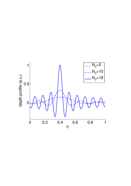
Fig. 2: Depth profile (left) and cross range profile (right) of the mean point spread function for the time reversal functional. Here $Z_{\mathcal{A}}=100$, $\ell=1$, $\sigma=0.25$, $k=60$, ${\mathcal{D}}=1$ (so that $N=19$). The array diameter $|{\mathcal{A}}_{X}|$ is supposed to be smaller than the critical value (127) which is about $220$. $N_{T}$ is the cut-off number (modes smaller than $N_{T}$ are recorded and reemitted). Note that the high modes play an important role. The larger $N_{T}$ is, the better the resolution.

7.3 Statistical stability

We now show that the time reversal function is statistically stable, meaning that the refocusing of the wave at the original source location does not depend on the the realization of the random medium but only on its statistical distribution, and the point spread function is approximately equal to its expectation.

We restrict the analysis of statistical stability to the case of full aperture, where the calculations are simpler because the coupling matrix $\Gamma_{jl}$ becomes the identity. The point spread function follows from (118)

$${\mathcal{M}}^{\tiny\mbox{TR}}({\omega},X^{s},\eta^{s})=\sum_{j=1}^{N}\frac{\phi_{j}(\eta^{s})\phi_{j}(\eta^{\star})}{\beta_{j}({\omega})}\psi\left(\frac{\beta^{\prime}_{j}({\omega})Z_{\mathcal{A}}}{T}\right)\int dX\,\frac{1_{{\mathcal{A}}_{X}}(X)}{|{\mathcal{A}}_{X}|}{\mathcal{T}}_{j}({\omega},X,X^{s},Z_{\mathcal{A}})\overline{{\mathcal{T}}_{j}({\omega},X,X^{\star},Z_{\mathcal{A}})},$$

and its variance at the source location is

$${\rm Var}\left[{\mathcal{M}}^{\tiny\mbox{TR}}({\omega},X^{\star},\eta^{\star})\right]=\sum_{j,J=1}^{N}\frac{\phi_{j}^{2}(\eta^{\star})}{\beta_{j}({\omega})}\frac{\phi_{J}^{2}(\eta^{\star})}{\beta_{J}({\omega})}\psi\left(\frac{\beta^{\prime}_{j}({\omega})Z_{\mathcal{A}}}{T}\right)\psi\left(\frac{\beta^{\prime}_{J}({\omega})Z_{\mathcal{A}}}{T}\right)\iint dXdY\,\frac{1_{{\mathcal{A}}_{X}}(X)1_{{\mathcal{A}}_{X}}(Y)}{|{\mathcal{A}}_{X}|^{2}}$$

$$\times\Big{\{}\mathbb{E}\big{[}\left|{\mathcal{T}}_{j}({\omega},X,X^{\star},Z_{\mathcal{A}})\right|^{2}\left|{\mathcal{T}}_{J}({\omega},Y,X^{\star},Z_{\mathcal{A}})\right|^{2}\big{]}-\mathbb{E}\big{[}\left|{\mathcal{T}}_{j}({\omega},X,X^{\star},Z_{\mathcal{A}})\right|^{2}\big{]}\mathbb{E}\big{[}\left|{\mathcal{T}}_{J}({\omega},Y,X^{\star},Z_{\mathcal{A}})\right|^{2}\big{]}\Big{\}}.$$

From appendix B (first case) we find that the variance is much smaller than the square expectation when $|A_{X}|\gg\ell$, and therefore the point spread function is equal to its mean approximately. The results contained in appendix B (second case) also show that if $|A_{X}|<\ell$, the variance of the point spread function is large, and therefore that time reversal refocusing may be unstable in this case.

There is however another mechanism that can ensure statistical stability of the focal spot if the array is small. Indeed, if the bandwidth of $\varphi$ is larger than the decorrelation frequency, then the variance

$${\rm Var}\left[{\cal J}^{\tiny\mbox{TR}}(X^{\star},\eta^{\star})\right]=\int\frac{d{\omega}}{2\pi}\int\frac{d{\omega}^{\prime}}{2\pi}\overline{\widehat{\varphi}({\omega},X)}\,\widehat{\varphi}({\omega}^{\prime})\,{\rm Cov}\big{[}{\mathcal{M}}^{\tiny\mbox{TR}}({\omega},X^{\star},\eta^{\star}),{\mathcal{M}}^{\tiny\mbox{TR}}({\omega}^{\prime},X^{\star},\eta^{\star})\big{]}$$

is small because the covariance of the point spread function at two frequencies becomes approximately zero if the frequency gap is large enough. Therefore, if the pulse has large bandwidth, then the time-reversal focal spot is statistically stable even for small arrays.

8 Imaging

The sharp and stable focusing of the time reversal process in the random waveguide is due the backpropagation of the time reversed field $D^{\tiny\mbox{TR}}$ in exactly the same waveguide. Time reversal is a physical experiment, where the waves can be observed in the vicinity of the source, as they refocus. In imaging we only have access to the data measured at the array, and the backpropagation to the search points is synthetic. Because we cannot know the fluctuations of the boundary, we simply ignore them in the synthetic backpropagation and obtain the so-called reversed time migration imaging function. We analyze it in section 8.1 and show that it does not give useful results in the low-SNR regime. In particular, we show that the images are not statistically stable with respect to realizations of the fluctuations. Stability can be achieved by imaging with local cross-correlations of the array measurements. Local means that we recall the decorrelation properties of the random mode amplitudes described in section 5.4, and cross-correlate the measurements over receivers located at nearby cross-ranges $X$, and projected on the same eigenfunctions. The resulting coherent interferometric imaging method is analyzed in section 8.2.

8.1 Reverse time migration

The reverse time migration function is given by the time reversed data $D^{\tiny\mbox{TR}}$ propagated (migrated) in the ideal waveguide to the search points $(x^{s},\eta^{s},z^{s})=\left(\frac{X^{s}}{\varepsilon},\eta^{s},\frac{Z^{s}}{\varepsilon^{2}}\right).$ Its mathematical expression follows from (25), with amplitudes (23) replaced by

$$a_{j,o}({\omega},X,Z)\leadsto\int dX^{\prime}{\mathcal{T}}_{j,o}({\omega},X,X^{\prime},Z)\frac{1}{2i\beta_{j}({\omega})}\int_{0}^{\mathcal{D}}d\eta\,\phi_{j}(\eta)\widehat{D}^{\tiny\mbox{TR}}({\omega},X^{\prime},\eta).$$ (135)

The ideal transfer coefficients

$${\mathcal{T}}_{j,o}({\omega},X,X^{\prime},Z)=\sqrt{\frac{\beta_{j}({\omega})}{2\pi iZ}}\exp\left[\frac{i\beta_{j}({\omega})(X-X^{\prime})^{2}}{2Z}\right]$$ (136)

are defined by the Green’s functions of the paraxial operator in (26). We obtain

$${\cal J}^{\tiny\mbox{M}}(X^{s},\eta^{s},Z^{s})=\sum_{j=1}^{N}\phi_{j}(\eta^{s})\int\frac{d{\omega}}{2\pi}\,\frac{\exp\left[i\beta_{j}({\omega})\frac{Z_{\mathcal{A}}-Z^{s}}{\varepsilon^{2}}-i{\omega}t\right]}{2i\beta_{j}({\omega})}\int dX\int d\eta\,\phi_{j}(\eta)$$

$$\times\,\widehat{D}^{\tiny\mbox{TR}}({\omega},X,\eta)\,{\mathcal{T}}_{j,o}({\omega},X,X^{s},Z_{\mathcal{A}}-Z^{s})\Big{|}_{t=T^{\varepsilon}},$$ (137)

with the right hand side evaluated at the same time $t=T_{\varepsilon}$ as in time reversal.

We assume again a tightly supported source density normalized by (105) and substitute the model (111) of $\widehat{D}^{\tiny\mbox{TR}}$ in (137) to obtain

$${\cal J}^{\tiny\mbox{M}}(X^{s},\eta^{s},Z^{s})=\int\frac{d{\omega}}{2\pi}\,\overline{\widehat{\varphi}({\omega})}\,{\mathcal{M}}^{\tiny\mbox{M}}\left({\omega},X^{s},\eta^{s},Z^{s}\right),$$ (138)

with frequency-dependent kernel (point spread function)

$${\mathcal{M}}^{\tiny\mbox{M}}\left({\omega},X^{s},\eta^{s},Z^{s}\right)\approx\sum_{j,l=1}^{N}\Gamma_{jl}\frac{\phi_{j}(\eta^{s})\phi_{l}(\eta^{\star})}{4\beta_{j}({\omega})\beta_{l}({\omega})}\int\frac{du}{2\pi}\,\overline{\widehat{\psi}(u)}\int dX\,1_{{\mathcal{A}}_{X}}(X)$$

$$\times{\mathcal{T}}_{j,o}\Big{(}{\omega},X,X^{s},Z_{\mathcal{A}}-Z^{s}\Big{)}\overline{{\mathcal{T}}_{l}\Big{(}{\omega}-\frac{\varepsilon^{2}u}{T},X,X^{\star},Z_{\mathcal{A}}\Big{)}}$$

$$\times\exp\left[i\beta_{j}({\omega})\frac{Z_{\mathcal{A}}-Z^{s}}{\varepsilon^{2}}-i\beta_{l}\Big{(}{\omega}-\frac{\varepsilon^{2}u}{T}\Big{)}\frac{Z_{\mathcal{A}}}{\varepsilon^{2}}\right].$$ (139)

8.1.1 The mean imaging function

Let us take for simplicity the case of full aperture in depth, where the coupling matrix $\Gamma_{jl}$ given by (114) becomes the identity. We obtain from (139) and the moment formula (74) that

$$\mathbb{E}\left[{\mathcal{M}}^{\tiny\mbox{M}}({\omega},X^{s},\eta^{s},Z^{s})\right]=\frac{|{\mathcal{A}}_{X}|}{8\pi Z_{\mathcal{A}}}\sum_{j=1}^{N}\frac{\phi_{j}(\eta^{s})\phi_{j}(\eta^{\star})}{\beta_{j}({\omega})}\psi\left(\frac{\beta^{\prime}_{j}({\omega})Z_{\mathcal{A}}}{T}\right)\exp\left[-\frac{Z_{\mathcal{A}}}{{\mathcal{S}}_{j}({\omega})}-i\beta_{j}({\omega})\frac{Z^{s}}{\varepsilon^{2}}\right]$$

$$\times\int dX\,\frac{1_{{\mathcal{A}}_{X}}(X)}{|{\mathcal{A}}_{X}|}\exp\left[-\frac{i\beta_{j}({\omega})}{Z_{\mathcal{A}}}\Big{(}X-\frac{X^{s}+X^{\star}}{2}\Big{)}(X^{s}-X^{\star})\right].~{}~{}$$ (140)

Moreover, assuming the aperture ${\mathcal{A}}_{X}$ defined in (121), and integrating in $X$, we get

$$\mathbb{E}\left[{\mathcal{M}}^{\tiny\mbox{M}}({\omega},X^{s},\eta^{s},Z^{s})\right]=\frac{|{\mathcal{A}}_{X}|}{8\pi Z_{\mathcal{A}}}\sum_{j=1}^{N}\frac{\phi_{j}(\eta^{s})\phi_{j}(\eta^{\star})}{\beta_{j}({\omega})}\psi\left(\frac{\beta^{\prime}_{j}({\omega})Z_{\mathcal{A}}}{T}\right)\exp\left[-\frac{Z_{\mathcal{A}}}{{\mathcal{S}}_{j}({\omega})}-i\beta_{j}({\omega})\frac{Z^{s}}{\varepsilon^{2}}\right]$$

$$\times\mbox{\rm sinc}\left[\frac{\beta_{j}({\omega})|{\mathcal{A}}_{X}|}{2Z_{\mathcal{A}}}(X^{s}-X^{\star})\right]\exp\left\{\frac{i\beta_{j}({\omega})}{2Z_{\mathcal{A}}}\left[(X^{s})^{2}-(X^{\star})^{2}\right]\right\}.~{}~{}$$ (141)

This result is almost the same as in the ideal waveguide, except for the damping coefficients $\exp\left[-Z_{\mathcal{A}}/{\mathcal{S}}_{j}\right].$

The sinc kernel in the mean point spread function gives the focusing in cross-range, with mode-dependent resolution

$$|X^{S}-X^{\star}|\leq\Delta_{X,j}({\omega})=\frac{2\pi Z_{\mathcal{A}}}{\beta_{j}({\omega})|{\mathcal{A}}_{X}|}.$$ (142)

The best resolution is for the first mode, that has the largest wavenumber $\beta_{1}({\omega})\approx{\pi N}/{{\mathcal{D}}}\approx k,$ and gives the Rayleigh cross-range resolution

$$\Delta_{X,1}({\omega})\approx\frac{2\pi Z_{\mathcal{A}}}{k|{\mathcal{A}}_{X}|}.$$ (143)

The focusing of the point spread function ${\mathcal{M}}^{\tiny\mbox{M}}$ in range can only be due to the summation of the rapidly oscillating terms $\exp\left[-i\beta_{j}Z^{s}/\varepsilon^{2}\right]$. But these terms are weighted by $\mbox{exp}[-Z_{\mathcal{A}}/{\mathcal{S}}_{j}]$, which decay fast in $j$. The first term dominates in

$$\mathbb{E}\left[{\mathcal{M}}^{\tiny\mbox{M}}({\omega},X^{\star},\eta^{\star},Z^{s})\right]=\frac{|{\mathcal{A}}_{X}|}{8\pi Z_{\mathcal{A}}}\sum_{j=1}^{N}\frac{\phi_{j}^{2}(\eta^{\star})}{\beta_{j}({\omega})}\psi\left(\frac{\beta^{\prime}_{j}({\omega})Z_{\mathcal{A}}}{T}\right)\exp\left[-\frac{Z_{\mathcal{A}}}{{\mathcal{S}}_{j}({\omega})}-i\beta_{j}({\omega})\frac{Z^{s}}{\varepsilon^{2}}\right],$$ (144)

so the mode diversity does not lead to focusing in range, as is the case in ideal waveguides. Nevertheless, the mean reverse time migration function peaks at $Z^{s}=0$ because of the integral over the bandwidth in

$$\mathbb{E}\left[{\cal J}^{\tiny\mbox{M}}(X^{\star},\eta^{\star},Z^{s})\right]=\int\frac{d{\omega}}{2\pi}\overline{\widehat{\varphi}({\omega})}\mathbb{E}\left[{\mathcal{M}}^{\tiny\mbox{M}}({\omega},X^{\star},\eta^{\star},Z^{s})\right],$$ (145)

and the range resolution is of the order $\varepsilon^{2}/[\beta^{\prime}_{1}({\omega}_{o})B]$.

When we evaluate the point spread function at $Z^{s}=0$ and $X^{s}=X^{\star}$, we obtain

$$\mathbb{E}\left[{\mathcal{M}}^{\tiny\mbox{M}}({\omega},X^{s}=X^{\star},\eta^{s},Z^{s}=0)\right]=\frac{|{\mathcal{A}}_{X}|}{8\pi Z_{\mathcal{A}}}\sum_{j=1}^{N}\frac{\phi_{j}(\eta^{s})\phi_{j}(\eta^{\star})}{\beta_{j}({\omega})}\psi\left(\frac{\beta^{\prime}_{j}({\omega})Z_{\mathcal{A}}}{T}\right)e^{-{Z_{\mathcal{A}}}/{{\mathcal{S}}_{j}({\omega})}}.\qquad$$ (146)

This is a sum of the oscillatory functions

$$\phi_{j}(\eta^{s})\phi_{j}(\eta^{\star})=\frac{1}{\mathcal{D}}\left\{\cos\left[\pi\left(j-\frac{1}{2}\right)\frac{(\eta^{s}-\eta^{\star})}{\mathcal{D}}\right]+\cos\left[\pi\left(j-\frac{1}{2}\right)\frac{(\eta^{s}+\eta^{\star})}{\mathcal{D}}\right]\right\}$$

multiplied by positive weights, which are small and decay fast in $j$. The first term dominates in (146) and there is no depth resolution at all. We show next that these small weights also indicate the lack of statistical stability of the reverse time migration function.

8.1.2 Stability analysis

To assess the stability of the reverse time migration, we calculate its variance at the source location

$$\mbox{Var}\left[{\cal J}^{\tiny\mbox{M}}(X^{\star},\eta^{\star},0)\right]=\mathbb{E}\left[\left|{\cal J}^{\tiny\mbox{M}}(X^{\star},\eta^{\star},0)\right|^{2}\right]-\left|\mathbb{E}\left[{\cal J}^{\tiny\mbox{M}}(X^{\star},\eta^{\star},0)\right]\right|^{2}.$$

We have from the results above that

$$\mathbb{E}\left[{\cal J}^{\tiny\mbox{M}}(X^{\star},\eta^{\star},0)\right]\approx\frac{|{\mathcal{A}}_{X}|}{8\pi Z_{\mathcal{A}}}\int\frac{d{\omega}}{2\pi}\,\overline{\widehat{\varphi}({\omega})}\sum_{j=1}^{N}\frac{\phi_{j}^{2}(\eta^{\star})}{\beta_{j}({\omega})}\psi\left(\frac{\beta^{\prime}_{j}({\omega})Z_{\mathcal{A}}}{T}\right)e^{-{Z_{\mathcal{A}}}/{{\mathcal{S}}_{j}({\omega})}}.$$ (147)

The second moment of ${\cal J}^{\tiny\mbox{M}}$ is

$$\mathbb{E}\left[\left|{\cal J}^{\tiny\mbox{M}}(X^{\prime},\eta^{\prime},0)\right|^{2}\right]\approx\int\frac{d{\omega}_{1}}{2\pi}\int\frac{d{\omega}_{2}}{2\pi}\,\overline{\varphi({\omega}_{1})}\varphi({\omega}_{2})\sum_{j,l=1}^{N}\frac{\phi_{j}^{2}(\eta^{\star})\phi_{l}^{2}(\eta^{\star})}{16\beta_{j}^{2}({\omega}_{1})\beta_{l}^{2}({\omega}_{2})}\int\frac{du_{1}}{2\pi}\int\frac{du_{2}}{2\pi}\,\overline{\widehat{\psi}(u_{1})}{\widehat{\psi}(u_{2})}~{}~{}$$

$$\times\,\exp\left[\frac{i[\beta^{\prime}_{j}({\omega}_{1})u_{1}-\beta^{\prime}_{l}({\omega}_{2})u_{2}]Z_{\mathcal{A}}}{T}\right]\int dX_{1}\int dX_{2}\,1_{{\mathcal{A}}_{X}}(X_{1})1_{{\mathcal{A}}_{X}}(X_{2})\,{\mathcal{T}}_{j,o}({\omega}_{1},X_{1},X^{\star},Z_{\mathcal{A}})~{}~{}$$

$$\times\,\overline{{\mathcal{T}}_{l,o}({\omega}_{1},X_{1},X^{\star},Z_{\mathcal{A}})}\mathbb{E}\left[\overline{{\mathcal{T}}_{j}\left({\omega}_{1}-\frac{\varepsilon^{2}u_{1}}{T},X_{1},X^{\star},Z_{\mathcal{A}}\right)}{\mathcal{T}}_{l}\left({\omega}_{2}-\frac{\varepsilon^{2}u_{2}}{T},X_{2},X^{\star},Z_{\mathcal{A}}\right)\right],~{}~{}$$ (148)

and we recall from Proposition 4 that only the diagonal terms $j=l$ contribute to the expectation. We also assume a small bandwidth $B\ll\Omega_{d,j}$, for all the modes $j$, so that we can use the simpler moment formula (98). We obtain

$$\mathbb{E}\left[\left|{\cal J}^{\tiny\mbox{M}}(X^{\prime},\eta^{\prime},0)\right|^{2}\right]\approx\frac{|\varphi(0)|^{2}}{(8\pi Z_{\mathcal{A}})^{2}}\sum_{j=1}^{N}\frac{\phi_{j}^{4}(\eta^{\star})}{\beta_{j}^{2}({\omega}_{o})}\left|\psi\left(\frac{\beta^{\prime}_{j}({\omega}_{o})Z_{\mathcal{A}}}{T}\right)\right|^{2}\int dX_{1}\int dX_{2}\,1_{{\mathcal{A}}_{X}}(X_{1})$$

$$\times\,1_{{\mathcal{A}}_{X}}(X_{2})\exp\left[-\frac{(X_{1}-X_{2})^{2}}{2X_{d,j}^{2}({\omega}_{o})}\right],$$ (149)

after approximating the modal wavenumbers by their value at the central frequency. This expression can be approximated further, after integrating in $X_{1}$ and $X_{2}$, and supposing that the decoherence lengths $X_{d,j}$ are much smaller than the array aperture,

$$\mathbb{E}\left[\left|{\cal J}^{\tiny\mbox{M}}(X^{\prime},\eta^{\prime},0)\right|^{2}\right]\approx\frac{|\varphi(0)|^{2}|{\mathcal{A}}_{X}|\sqrt{2\pi}}{(8\pi Z_{\mathcal{A}})^{2}}\sum_{j=1}^{N}\frac{X_{d,j}({\omega}_{o})\phi_{j}^{4}(\eta^{\star})}{\beta_{j}^{2}({\omega}_{o})}\left|\psi\left(\frac{\beta^{\prime}_{j}({\omega}_{o})Z_{\mathcal{A}}}{T}\right)\right|^{2}.$$ (150)

The second moment (150) is clearly much larger than the square of the mean (147), which is exponentially small in range. Although the mean of the imaging function is focused at the source, it cannot be observed because it is dominated by its random fluctuations. The reverse time migration lacks statistical stability with respect to the realizations of the random fluctuations of the boundary of the waveguide.

The calculations above are for a small bandwidth, satisfying $B\ll\Omega_{d,j}$ for all the modes captured in the recording window. The calculations are more complicated for a larger bandwidth, but the conclusion remains that reverse time migration is not stable with respect to different realization of the random boundary fluctuations.

8.2 Coherent interferometric imaging

The main idea of the coherent interferometric (CINT) imaging approach is to backpropagate synthetically to the imaging points the local cross-correlations of the array measurements, instead of the measurements themselves. By local we mean that because of the statistical decorrelation properties of the random mode amplitudes described in section 5.4, we cross-correlate the data $\widehat{D}({\omega},X,\eta)$ at nearby frequencies and cross-ranges $X$, after projecting it on the subspace of one eigenfunction $\phi_{j}$ at a time. The projection gives the coefficients

$$\widehat{D}_{j}({\omega},X)=\int_{0}^{{\mathcal{D}}}d\eta\,\phi_{j}(\eta)\widehat{D}({\omega},X,\eta),$$ (151)

which are directly proportional to the coefficients $\widehat{F}_{j}$ of the source only in the case of an array spanning the entire depth of the waveguide. We assume this case here, because it simplifies the analysis of the focusing and stability of the CINT function. We also take a small source, meaning that we essentially compute the CINT point spread function.

The model of the coefficients (151) is

$$\widehat{D}_{j}({\omega},X)\approx 1_{{\mathcal{A}}_{X}}(X)\frac{\widehat{\varphi}({\omega})\phi_{j}(\eta^{\star})}{2i\beta_{j}({\omega})}e^{i\beta_{j}({\omega})Z_{\mathcal{A}}/\varepsilon^{2}}\int\frac{du}{2\pi}\,\widehat{\psi}(u)e^{-i\beta^{\prime}_{j}({\omega})uZ_{\mathcal{A}}/T}{\mathcal{T}}_{j}\Big{(}{\omega}-\frac{\varepsilon^{2}u}{T},X,X^{\star},Z_{\mathcal{A}}\Big{)},$$ (152)

and we cross-correlate them at cross-ranges satisfying $|X_{1}-X_{2}|\leq X_{d,j}({\omega}),$ and at frequency offsets

$$|{\omega}_{1}-{\omega}_{2}|\leq\Omega\ll\Omega_{d,j}.$$ (153)

We take such small $\Omega$ to simplify the second moment formulas.

The CINT image is formed by backpropagating the cross-correlations to the imaging point, using the Green’s function in the ideal waveguide. We first define the CINT image in the $(X,Z)$-domain:

$${\cal J}^{\tiny\mbox{CINT}}(X^{s},Z^{s})=\sum_{j=1}^{N}{\cal J}^{\tiny\mbox{CINT}}_{j}(X^{s},Z^{s})$$ (154)

with

$${\cal J}^{\tiny\mbox{CINT}}_{j}(X^{s},Z^{s}) = \iint\frac{d{\omega}_{1}}{2\pi}\frac{d{\omega}_{2}}{2\pi}1_{\Omega}({\omega}_{1}-{\omega}_{2})e^{i[\beta_{j}({\omega}_{2})-\beta_{j}({\omega}_{1})]\frac{Z^{s}-Z_{\mathcal{A}}}{\varepsilon^{2}}}\iint dX_{1}dX_{2}\,1_{X_{d,j}}(X_{1}-X_{2})$$ (155)

$$\times\,\widehat{D}_{j}({\omega}_{1},X_{1})\overline{\widehat{D}_{j}({\omega}_{2},X_{2})}\overline{{\mathcal{T}}_{j,o}\Big{(}{\omega}_{1},X_{1},X^{s},Z_{\mathcal{A}}-Z^{s}\Big{)}}{\mathcal{T}}_{j,o}\Big{(}{\omega}_{2},X_{2},X^{s},Z_{\mathcal{A}}-Z^{s}\Big{)},\quad$$

where $1_{X_{d,j}}$ are indicator functions of the cross-range interval $\left[-X_{d,j}({\omega}),X_{d,j}({\omega})\right]$ calculated at the central frequency ${\omega}=({\omega}_{1}+{\omega}_{2})/{2}.$ Similarly, $1_{\Omega}$ is the indicator function of the frequency interval $[-\Omega,\Omega]$.

8.2.1 The mean CINT function

To study the focusing of CINT, we consider its expectation

$$\mathbb{E}\left[{\cal J}^{\tiny\mbox{CINT}}(X^{s},Z^{s})\right]\approx\int\frac{d{\omega}}{2\pi}\left|\widehat{\varphi}({\omega})\right|^{2}\mathbb{E}\left[{\mathcal{M}}^{\tiny\mbox{CINT}}({\omega},X^{s},Z^{s})\right],$$ (156)

with frequency-dependent kernel

$$\mathbb{E}\left[{\mathcal{M}}^{\tiny\mbox{CINT}}({\omega},X^{s},Z^{s})\right]\approx\sum_{j=1}^{N}\frac{\phi_{j}^{2}(\eta^{\star})}{32\pi^{3}Z_{\mathcal{A}}(Z_{\mathcal{A}}-Z^{s})}\left|\psi\left(\frac{\beta^{\prime}_{j}({\omega})Z_{\mathcal{A}}}{T}\right)\right|^{2}\iint dX_{1}dX_{2}\,1_{{\mathcal{A}}_{X}}(X_{1})1_{{\mathcal{A}}_{X}}(X_{2})$$

$$\times\exp\left\{i\beta_{j}({\omega})\left[\frac{(X_{1}-X^{\star})^{2}}{2Z_{\mathcal{A}}}-\frac{(X_{1}-X^{s})^{2}}{2(Z_{\mathcal{A}}-Z^{s})}-\frac{(X_{2}-X^{\star})^{2}}{2Z_{\mathcal{A}}}+\frac{(X_{2}-X^{s})^{2}}{2(Z_{\mathcal{A}}-Z^{s})}\right]-\frac{(X_{1}-X_{2})^{2}}{2X_{d,j}^{2}({\omega})}\right\}$$

$$\times\int\frac{d\widetilde{\omega}}{2\pi}\,1_{\Omega}(\widetilde{\omega})\exp\left\{i\left[\beta_{j}\left({\omega}+\frac{\widetilde{\omega}}{2}\right)-\beta_{j}\left({\omega}-\frac{\widetilde{\omega}}{2}\right)\right]\frac{Z^{s}}{\varepsilon^{2}}\right\}.~{}~{}~{}~{}$$ (157)

This expression follows from (155), the second moment formula (98), and definition (136) of the ideal transfer coefficients ${\mathcal{T}}_{j,o}$.

8.2.2 Cross-range focusing

Let us consider in (157) a search point at the range of the source $Z^{s}=0$,

$$\mathbb{E}\left[{\mathcal{M}}^{\tiny\mbox{CINT}}({\omega},X^{s},0)\right]\approx\frac{\Omega}{64\pi^{4}Z^{2}_{\mathcal{A}}}\sum_{j=1}^{N}\phi_{j}^{2}(\eta^{\star})\left|\psi\left(\frac{\beta^{\prime}_{j}({\omega})Z_{\mathcal{A}}}{T}\right)\right|^{2}\iint dX_{1}dX_{2}\,1_{{\mathcal{A}}_{X}}(X_{1})1_{{\mathcal{A}}_{X}}(X_{2})$$

$$\times\exp\left[i\beta_{j}({\omega})\frac{(X^{s}-X^{\star})}{Z_{\mathcal{A}}}(X_{1}-X_{2})-\frac{(X_{1}-X_{2})^{2}}{2X_{d,j}^{2}({\omega})}\right].\quad$$ (158)

This formula simplifies after integrating over the array aperture and assuming as before that $X_{d,j}\ll|{\mathcal{A}}_{X}|$,

$$\mathbb{E}\left[{\mathcal{M}}^{\tiny\mbox{CINT}}({\omega},X^{s},0)\right]\sim\frac{\Omega|{\mathcal{A}}_{X}|(2\pi)^{1/2}}{64\pi^{4}Z^{2}_{\mathcal{A}}}\sum_{j=1}^{N}\phi_{j}^{2}(\eta^{\star})X_{d,j}({\omega})\left|\psi\left(\frac{\beta^{\prime}_{j}({\omega})Z_{\mathcal{A}}}{T}\right)\right|^{2}$$

$$\times\,\exp\left\{-\frac{1}{2}\left[\frac{\beta_{j}({\omega})(X^{s}-X^{\star})X_{d,j}({\omega})}{Z_{\mathcal{A}}}\right]^{2}\right\}.$$ (159)

Each term in the sum focuses at the source, with resolution

$$|X^{s}-X^{\star}|\leq\Delta_{X,j}({\omega})=\frac{2Z_{\mathcal{A}}}{\beta_{j}({\omega})X_{d,j}({\omega})}$$ (160)

defined as twice the standard deviation of the Gaussian in (159). The number of modes participating in the sum is determined by the length of the recording time window, as before, but each mode is weighted by the correlation length $X_{d,j}$, which decreases monotonically with $j$. The first mode has the largest contribution in (159), and gives the best cross-range resolution. Since its wavenumber is approximately $\beta_{1}({\omega})\approx\pi N/{\mathcal{D}}\approx k$,

$$\Delta_{X,1}({\omega})\approx\frac{2Z_{\mathcal{A}}}{kX_{d,j}({\omega})}\sim\frac{2\pi Z_{\mathcal{A}}}{k\left[\pi X_{d,1}({\omega})\right]}$$ (161)

is comparable to the classic Rayleigh resolution for an array of aperture equal to $\pi X_{d,1}({\omega})$ (see Figure 3).

The cross-range resolution (161) is worse than that of time reversal. Scattering at the random boundary is beneficial to the time reversal process, and the more modes are recorded, the better the result. However, scattering impedes imaging, and the best cross-range resolution is achieved with the first mode. Even with this mode, the resolution is worse than that in ideal waveguides $2\pi Z_{\mathcal{A}}/(k|{\mathcal{A}}_{X}|)$, because $X_{d,1}\ll|{\mathcal{A}}_{X}|$.

8.2.3 Range focusing

When we evaluate the mean CINT point spread function (157) at the cross-range $X^{s}=X^{\star}$, we obtain

$$\mathbb{E}\left[{\mathcal{M}}^{\tiny\mbox{CINT}}({\omega},X^{\star},Z^{s})\right]\approx\sum_{j=1}^{N}\frac{\phi_{j}^{2}(\eta^{\star})}{32\pi^{3}Z_{\mathcal{A}}(Z_{\mathcal{A}}-Z^{s})}\left|\psi\left(\frac{\beta^{\prime}_{j}({\omega})Z_{\mathcal{A}}}{T}\right)\right|^{2}\iint dX_{1}dX_{2}\,1_{{\mathcal{A}}_{X}}(X_{1})1_{{\mathcal{A}}_{X}}(X_{2})$$

$$\times\exp\left\{-i\beta_{j}({\omega})\frac{(X_{1}-X_{2})Z^{s}}{Z_{\mathcal{A}}(Z_{\mathcal{A}}-Z^{s})}\left(\frac{X_{1}+X_{2}}{2}-X^{\star}\right)-\frac{(X_{1}-X_{2})^{2}}{2X_{d,j}^{2}({\omega})}\right\}$$

$$\times\int\frac{d\widetilde{\omega}}{2\pi}\,1_{\Omega}(\widetilde{\omega})\exp\left\{-i\left[\beta_{j}\left({\omega}+\frac{\widetilde{\omega}}{2}\right)-\beta_{j}\left({\omega}-\frac{\widetilde{\omega}}{2}\right)\right]\frac{Z^{s}}{\varepsilon^{2}}\right\}.~{}~{}~{}~{}$$ (162)

Because we integrate over $\widetilde{\omega}$ the rapidly oscillating integrand, at scale $\varepsilon^{2}$, we have from the method of stationary phase that (162) is large for

$$Z^{s}=\varepsilon^{2}\zeta^{s}$$

with $\zeta^{s}$ independent of $\varepsilon$. Recall the assumption (153) of the frequency offsets.

The mean point spread function becomes

$$\mathbb{E}\left[{\mathcal{M}}^{\tiny\mbox{CINT}}({\omega},X^{\star},\varepsilon^{2}\zeta^{s})\right]\approx\frac{\Omega|{\mathcal{A}}_{X}|(2\pi)^{1/2}}{64\pi^{4}Z_{\mathcal{A}}^{2}}\sum_{j=1}^{N}X_{d,j}({\omega})\phi_{j}^{2}(\eta^{\star})\left|\psi\left(\frac{\beta^{\prime}_{j}({\omega})Z_{\mathcal{A}}}{T}\right)\right|^{2}\mbox{sinc}\left[\beta^{\prime}_{j}({\omega})\Omega\zeta^{s}\right],\quad$$ (163)

and we define the mode-dependent scaled range resolution by

$$|\zeta^{s}|\leq\Delta_{\zeta,j}=\frac{1}{\Omega\beta_{j}^{\prime}({\omega})}.$$ (164)

Again, the resolution is best for the first mode, which has the largest weight $X_{d,1}({\omega})$ in (163). See Figure 3 for an illustration.

8.2.4 Depth estimation

One natural way to estimate the depth $\eta^{\star}$ would be to consider the full CINT imaging functional

$$\widetilde{\cal J}^{\tiny\mbox{CINT}}(X^{s},\eta^{s},Z^{s})=\sum_{j=1}^{N}{\cal J}^{\tiny\mbox{CINT}}_{j}(X^{s},Z^{s})\phi_{j}^{2}(\eta^{s}),$$

with ${\cal J}^{\tiny\mbox{CINT}}_{j}(X^{s},Z^{s})$ defined by (155). However, if we define $\widetilde{\mathcal{M}}^{\tiny\mbox{CINT}}$ as

$$\mathbb{E}\left[\widetilde{\cal J}^{\tiny\mbox{CINT}}(X^{s},\eta^{s},Z^{s})\right]\approx\int\frac{d{\omega}}{2\pi}\left|\widehat{\varphi}({\omega})\right|^{2}\mathbb{E}\left[\widetilde{\mathcal{M}}^{\tiny\mbox{CINT}}({\omega},X^{s},\eta^{s},Z^{s})\right],$$ (165)

and if we take $X^{s}=X^{\star}$ and $Z^{s}=0$, then we obtain

$$\mathbb{E}\left[\widetilde{\mathcal{M}}^{\tiny\mbox{CINT}}({\omega},X^{\star},\eta^{s},0)\right]\approx\frac{\Omega|{\mathcal{A}}_{X}|(2\pi)^{1/2}}{64\pi^{4}Z_{\mathcal{A}}^{2}}\sum_{j=1}^{N}X_{d,j}({\omega})\phi_{j}^{2}(\eta^{\star})\phi_{j}^{2}(\eta^{s})\left|\psi\left(\frac{\beta^{\prime}_{j}({\omega})Z_{\mathcal{A}}}{T}\right)\right|^{2}.$$ (166)

This is a sum of positive terms and it does not have a peak at the depth of the source (see Figure 4).

Because of scattering at the random boundary the modes are decoupled, and we cannot speak of coherent imaging in depth. We work instead with the squares of the mode amplitudes, i.e. intensities. Incoherent imaging means estimating the depth of the source based on the mathematical model (166). More explicitly, we can estimate $\eta^{\star}$ by solving the least squares minimization problem

$$\min_{\eta^{s}}\sum_{j=1}^{N}\left|{\cal J}^{\tiny\mbox{CINT}}_{j}(\widehat{X}^{\star},\widehat{Z}^{\star})-\frac{\Omega|{\mathcal{A}}_{X}|(2\pi)^{1/2}}{64\pi^{4}Z_{\mathcal{A}}^{2}}\int\frac{d{\omega}}{2\pi}|\widehat{\varphi}({\omega})|^{2}X_{d,j}({\omega})\phi_{j}^{2}(\eta^{s})\left|\psi\left(\frac{\beta^{\prime}_{j}({\omega})Z_{\mathcal{A}}}{T}\right)\right|^{2}\right|^{2},$$ (167)

where the estimators $\widehat{X}^{\star}$ and $\widehat{Z}^{\star}$ of the cross-range $X^{\star}$ and range offset $Z^{\star}=0$ of the source have been determined as the location of the maximum of (154) (see Figure 4).

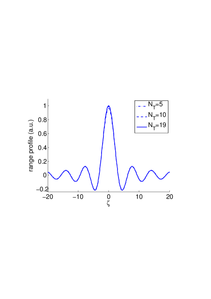
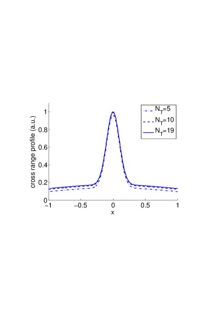
Fig. 3: Range profile and cross range profile of the mean point spread function for the CINT functional. Here $Z_{\mathcal{A}}=100$, $\ell=1$, $\sigma=0.25$, $k=60$, ${\mathcal{D}}=1$ (so that $N=19$), and the cut-off frequency is $\Omega/c=1$. $N_{T}$ is the cut-off number (modes smaller than $N_{T}$ are recorded and reemitted). Note that the high modes do not play any role.

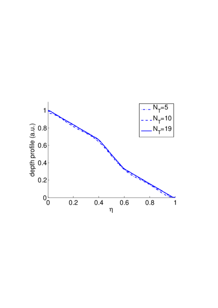
Fig. 4: Depth profile with (165) (left) and with (167) (right) for the CINT functional. In the right picture we plot the reciprocal of the square root of the function in (167). Here $Z_{\mathcal{A}}=100$, $\ell=1$, $\sigma=0.25$, $k=60$, ${\mathcal{D}}=1$ (so that $N=19$). $N_{T}$ is the cut-off number (modes smaller than $N_{T}$ are recorded and reemitted). Note that the high modes do not play any role.

8.2.5 Statistical stability

The analysis of statistical stability of the CINT function is basically the same as that of time reversal. The function is stable when evaluated in the vicinity of the source location if the array has large aperture $|{\mathcal{A}}_{X}|\gg\ell$. We have seen in section 8.2.2 that a large aperture does not improve the focusing of $\mathbb{E}\left[{\cal J}^{\tiny\mbox{CINT}}\right]$. The cross-range resolution is limited by the decoherence length. But a large aperture is needed for the CINT function to be statistically stable.

Another way of achieving statistical stability of CINT is to have a pulse with large bandwidth. This was already noted in the discussion of statistical stability of time reversal in section 7.3.

Note that the statistical stability of CINT relies on computing correctly the local cross-correlations of the measurements at the array. By this we mean that the cross-range and frequency offsets in the correlations should not exceed the decoherence length and frequency. Moreover, the cross-correlations should be with one mode at a time. This can be done with arrays that span the whole depth of the waveguide, because the coupling matrix $\Gamma_{jl}$ becomes the identity when $|{\mathcal{A}}_{\eta}|={\mathcal{D}}$. If the aperture $|{\mathcal{A}}_{\eta}|$ is small, there are large mode index offsets $|j-l|$ for which $\Gamma_{jl}\neq 0$. Consequently, there are many terms of the form $\overline{{\mathcal{T}}_{j}}{\mathcal{T}}_{l}$, with $j\neq l$, that participate in the expression of the imaging function. Since only the diagonal terms are correlated, we obtain that ${\cal J}^{\tiny\mbox{CINT}}$ has large variance when $|{\mathcal{A}}_{\eta}|\ll{\mathcal{D}}$.

In practice, the decoherence scales $X_{d,j}$ and $\Omega_{d,j}$ are likely not known explicitly. The formulas derived above are specific to our mathematical model. However, the decoherence scales can be estimated as we form the image, using an adaptive procedure similar to that introduced in [3].

9 Summary

In this paper we analyze propagation of acoustic waves in three-dimensional random waveguides. The waves are trapped by top and bottom boundaries, but the medium is unbounded in the remaining two directions. The top boundary has small, random fluctuations. We consider a source that emits a beam, and study the resulting random wave field in the waveguide.

The analysis is in a long range, paraxial scaling regime modeled with a small parameter $\varepsilon$. It is defined as the ratio of the central wavelength ${\lambda}_{o}$ of the pulse emitted from the source and the emitted beam width $r_{0}$. The range of propagation is of the order of the Rayleigh length $r_{0}^{2}/{\lambda}_{o}=\varepsilon^{-2}{\lambda}_{o}$. The fluctuations of the boundary are on a length scale that is similar to the beam width, and their small amplitude is scaled so that they cause significant cumulative scattering effects when the waves travel at ranges of the order of the Rayleigh length.

The wave field is given by a superposition of waveguide modes with random amplitudes. The modes are solutions of the wave equation in the ideal waveguide, with flat boundary. The scattering effects are captured by their random amplitudes. We show that in our scaling regime the amplitudes satisfy a system of paraxial equations driven by the same Brownian motion field. We use the system to calculate three important mode-dependent scales that quantify the net scattering effects in the waveguide, and play a key role in applications such as imaging and time reversal. The first mode-dependent scale is the scattering mean free path. It gives the range over which the mode loses its coherence, meaning that the expectation of its random amplitude is smaller than its fluctuations. The other mode-dependent scales are the decoherence length and frequency. They give the cross-range scale and frequency offsets over which the mode amplitudes become statistically uncorrelated.

We use the results of the analysis to study time reversal and imaging of the source with a remote array of sensors, in a low SNR regime. Low SNR means that the waves travel over distances that exceed the scattering mean free paths of all the modes, so that the random wave field measured at the array is dominated by its fluctuations.

In time reversal, the waves received at the array are time reversed and then re-emitted in the medium. They travel back to the source and refocus. The refocusing is expected by the time reversibility of the wave equation, but the resolution is limited in ideal waveguides by the aperture of the array. We analyze the time reversal process in the random waveguide and show that super-resolution occurs, meaning that scattering at the random boundary improves the refocusing resolution. An essential part of the resolution analysis is the assessment of statistical stability with respect to different realizations of the random boundary fluctuations. We show that statistical stability holds if the array has large aperture and/or the emitted pulse from the source has a large bandwidth.

Time reversal is very different from imaging. In time reversal the array measurements are backpropagated physically, in the real waveguide. In imaging we can only backpropagate the time reversed data in software, in a surrogate waveguide. Because we cannot know the boundary fluctuations, we neglect them altogether, and the surrogate is the ideal waveguide. The resulting imaging function is called reverse time migration and it does not work in low SNR regimes. It lacks statistical stability, i.e., the images change unpredictably from one realization of the fluctuations to another.

We show that robust imaging can be carried out in low SNR regimes if we backpropagate local cross-correlations of the array measurements, instead of the measurements themselves. Here local means that we cross-correlate the data projected on one mode at a time, and for nearby cross-ranges and frequencies. The method is called coherent interferometric (CINT), because it is an extension of the CINT approach introduced and analyzed in [5, 3, 4, 2] for imaging in open, random environments. We show that CINT images are statistically stable under two conditions: The first condition is the same as in time reversal and it says that the array should have a large aperture and/or the pulse bandwidth should be large. The second condition is that the cross-range and frequency offsets used in the calculation of the local cross-correlations do not exceed the mode-dependent decoherence length and frequency, respectively. We derived mathematical expressions of these scales, for our model. In practice, they can be estimated adaptively, using the image formation, with an approach similar to that in [3]. The estimation is possible because there is a trade-off between stability and resolution that is quantified by the decoherence scales. If we over-estimate them we lose statistical stability. If we under-estimate them, we lose resolution.

While cumulative scattering aids in time reversal, it impedes imaging. We quantify this explicitly in the resolution analysis of CINT. In time reversal the resolution improves when we record the wave field over a long time, so that we include the high-order modes that travel at slower speed. In CINT, the best cross-range and range resolution is given by the first mode, which encounters the random boundary less often, and is thus less affected by the fluctuations. The cross-range resolution is similar to the classic Rayleigh one of range times wavelength divided by the aperture, but instead of the real aperture we have the decoherence length of the mode. This length decreases monotonically with range, because longer distances of propagation in the random waveguide mean stronger scattering effects. Similarly, the range resolution is similar to the classic one, of speed divided by the bandwidth, but the bandwidth is replaced by the decoherence frequency which decreases monotonically with range.

The estimation of the depth of the source is different than that of range and cross-range. Because the modes decorrelate in the low SNR regime, we cross-correlate the data projected on one mode at a time, so essentially, we work with intensities. The estimation of the depth of the source from the intensities can be done by minimizing the misfit between the processed measurements and the mathematical model. While the cross-range and range estimation with CINT is done best with the first waveguide mode, the depth estimation requires many modes. Thus, we still need a long recording time at the array to capture the later arrival of the high-order modes.

10 Acknowledgements

The work of L. Borcea was partially supported by the AFSOR Grant FA9550-12-1-0117, the ONR Grants N00014-12-1-0256, N00014-09-1-0290 and N00014-05-1-0699, and by the NSF Grants DMS-0907746, DMS-0934594. The work of J.Garnier was supported in part by ERC Advanced Grant Project MULTIMOD-267184.

Appendix A Second moment calculation

The equation for $\mathbb{E}\left[{\mathcal{T}}_{j}({\omega}_{1},X_{1},X_{1}^{\prime},Z)\overline{{\mathcal{T}}_{l}}({\omega}_{2},X_{2},X_{2}^{\prime},Z)\right]$ follows from (68), using Itô calculus,

$$\partial_{Z}\mathbb{E}\left[{\mathcal{T}}_{j}\overline{{\mathcal{T}}_{l}}\right]=\left[\frac{i}{2\beta_{j}({\omega}_{1})}\partial_{X_{1}}^{2}-\frac{i}{2\beta_{l}({\omega}_{2})}\partial_{X_{2}}^{2}-\Big{(}\frac{1}{\sqrt{{\mathcal{S}}_{j}({\omega}_{1})}}-\frac{1}{\sqrt{{\mathcal{S}}_{l}({\omega}_{2})}}\Big{)}^{2}-\frac{2C_{o}(X_{1}-X_{2})}{\sqrt{{\mathcal{S}}_{j}({\omega}_{1}){\mathcal{S}}_{l}({\omega}_{2})}}\right]\mathbb{E}\left[{\mathcal{T}}_{j}\overline{{\mathcal{T}}_{l}}\right].~{}~{}$$ (168)

Its solution can be written as

$$\mathbb{E}\left[{\mathcal{T}}_{j}({\omega}_{1},X_{1},X_{1}^{\prime},Z)\overline{{\mathcal{T}}_{l}({\omega}_{2},X_{2},X_{2}^{\prime},Z)}\right]=M_{jl}({\omega}_{1},{\omega}_{2},X_{1},X_{2},Z;X_{1}^{\prime},X_{2}^{\prime})e^{-\Big{(}\frac{1}{\sqrt{{\mathcal{S}}_{j}({\omega}_{1})}}-\frac{1}{\sqrt{{\mathcal{S}}_{l}({\omega}_{2})}}\Big{)}^{2}Z},$$ (169)

with $M_{jl}$ solving

$$\partial_{Z}M_{jl}=\left[\frac{i}{2\beta_{j}({\omega}_{1})}\partial_{X_{1}}^{2}-\frac{i}{2\beta_{l}({\omega}_{2})}\partial_{X_{2}}^{2}-\frac{2C_{o}(X_{1}-X_{2})}{\sqrt{{\mathcal{S}}_{j}({\omega}_{1}){\mathcal{S}}_{l}({\omega}_{2})}}\right]M_{jl}$$ (170)

for $Z>0$, and the initial condition

$$M_{jl}({\omega}_{1},{\omega}_{2},X_{1},X_{2},0;X_{1}^{\prime},X_{2}^{\prime})=\delta(X_{1}-X_{1}^{\prime})\delta(X_{2}-X_{2}^{\prime}).$$ (171)

A.1 Single frequency

Let us begin with the single frequency case, ${\omega}_{1}={\omega}_{2}={\omega}$, and introduce the center and difference coordinates $\xi$ and $\widetilde{\xi}$ so that

$$X_{1}=\frac{\xi+\widetilde{\xi}/2}{\sqrt{\beta_{j}({\omega})}},\quad X_{2}=\frac{\xi-\widetilde{\xi}/2}{\sqrt{\beta_{l}({\omega})}}.$$ (172)

In this coordinate system we have that

$$U_{jl}({\omega},\xi,\widetilde{\xi},Z;\xi^{\prime},\widetilde{\xi}^{\prime})=M_{jl}\Big{(}{\omega},{\omega},\frac{\xi+\widetilde{\xi}/2}{\sqrt{\beta_{j}({\omega})}},\frac{\xi-\widetilde{\xi}/2}{\sqrt{\beta_{l}({\omega})}},Z;\frac{\xi^{\prime}+\widetilde{\xi}^{\prime}/2}{\sqrt{\beta_{j}({\omega})}},\frac{\xi^{\prime}-\widetilde{\xi}^{\prime}/2}{\sqrt{\beta_{l}({\omega})}}\Big{)}$$ (173)

satisfies the initial value problem

$$\partial_{Z}U_{jl} = i\partial_{\xi}\partial_{\widetilde{\xi}}U_{jl}-\frac{2}{\sqrt{{\mathcal{S}}_{j}{\mathcal{S}}_{l}}}C_{o}\Big{[}\Big{(}\frac{1}{\sqrt{\beta_{j}}}-\frac{1}{\sqrt{\beta_{l}}}\Big{)}\xi+\Big{(}\frac{1}{\sqrt{\beta_{j}}}+\frac{1}{\sqrt{\beta_{l}}}\Big{)}\frac{\widetilde{\xi}}{2}\Big{]}U_{jl},\qquad Z>0,$$

$$U_{jl} = \sqrt{\beta_{j}\beta_{l}}\,\delta(\xi-\xi^{\prime})\delta(\widetilde{\xi}-\widetilde{\xi}^{\prime}),\qquad Z=0.$$ (174)

Its Fourier transform in $\widetilde{\xi}$ is the Wigner distribution

$$W_{jl}({\omega},\xi,\widetilde{\kappa},Z;\xi^{\prime},\widetilde{\xi}^{\prime})=\int_{-\infty}^{\infty}\frac{d\widetilde{\xi}}{2\pi}\,U_{jl}({\omega},\xi,\widetilde{\xi},Z;\xi^{\prime},\widetilde{\xi}^{\prime})e^{-i\widetilde{\kappa}\widetilde{\xi}},$$ (175)

the solution of the transport equation

$$\left[\partial_{Z}+\widetilde{\kappa}\partial_{\xi}\right]W_{jl}({\omega},\xi,\widetilde{\kappa},Z;\xi^{\prime},\widetilde{\xi}^{\prime})=-\frac{4\sqrt{\beta_{l}}}{\sqrt{{\mathcal{S}}_{j}{\mathcal{S}}_{l}}(\sqrt{\beta_{j}}+\sqrt{\beta_{l}})}\int dq\,\widehat{C}_{o}\Big{(}q\frac{2\sqrt{\beta_{l}}}{(\sqrt{\beta_{j}}+\sqrt{\beta_{l}})}\Big{)}$$

$$\times\exp\left[-\frac{iq\xi}{\sqrt{\beta_{j}}}\frac{2(\sqrt{\beta_{j}}-\sqrt{\beta_{l}})}{(\sqrt{\beta_{j}}+\sqrt{\beta_{l}})}\right]W_{jl}\Big{(}{\omega},\xi,\widetilde{\kappa}-\frac{q}{\sqrt{\beta_{j}}},Z;\xi^{\prime},\widetilde{\xi}^{\prime}\Big{)},$$ (176)

for $Z>0$, with initial condition

$$W_{jl}({\omega},\xi,\widetilde{\kappa},0;\xi^{\prime},\widetilde{\xi}^{\prime})=\frac{\sqrt{\beta_{j}\beta_{l}}}{2\pi}e^{-i\widetilde{\kappa}\widetilde{\xi}^{\prime}}\delta(\xi-\xi^{\prime}),$$ (177)

and kernel

$$\widehat{C}_{o}(\kappa)=\delta(\kappa)-\frac{\widehat{R}_{o}(\kappa)}{R_{o}(0)}.$$ (178)

Here

$$\widehat{R}_{o}(\kappa)=\frac{1}{2\pi}\int R_{o}(\xi)e^{-i\kappa\cdot\xi}d\xi.$$

A.1.1 Single mode moments

The transport equation (176) simplifies in the case $j=l$,

$$\left[\partial_{Z}+\widetilde{\kappa}\partial_{\xi}\right]W_{jj}({\omega},\xi,\widetilde{\kappa},Z;\xi^{\prime},\widetilde{\xi}^{\prime}) = -\frac{2}{{\mathcal{S}}_{j}}\int dq\,\widehat{C}_{o}(q)W_{jl}\Big{(}{\omega},\xi,\widetilde{\kappa}-\frac{q}{\sqrt{\beta_{j}}},Z;\xi^{\prime},\widetilde{\xi}^{\prime}\Big{)},$$

$$W_{jj}({\omega},\xi,\widetilde{\kappa},0;\xi^{\prime},\widetilde{\xi}^{\prime}) = \frac{\beta_{j}}{2\pi}e^{-i\widetilde{\kappa}\widetilde{\xi}^{\prime}}\delta(\xi-\xi^{\prime}),$$ (179)

and can be integrated easily after Fourier transforming in $\widetilde{\kappa}$ and $\xi$. Explicitly,

$$V_{jj}({\omega},\kappa,\widetilde{\xi},Z;\xi^{\prime},\widetilde{\xi}^{\prime})=\int_{-\infty}^{\infty}\frac{d\xi}{2\pi}\int_{-\infty}^{\infty}d\widetilde{\kappa}\,W_{jj}({\omega},\xi,\widetilde{\kappa},Z;\xi^{\prime},\widetilde{\xi}^{\prime})e^{-i\kappa\xi+i\widetilde{\kappa}\widetilde{\xi}}$$ (180)

satisfies the initial value problem

$$\left[\partial_{Z}+\kappa\partial_{\widetilde{\xi}}\right]V_{jj}({\omega},\kappa,\widetilde{\xi},Z;\xi^{\prime},\widetilde{\xi}^{\prime}) = -\frac{2}{{\mathcal{S}}_{j}}{C}_{o}\Big{(}\frac{\widetilde{\xi}}{\sqrt{\beta_{j}}}\Big{)}V_{jj}({\omega},\kappa,\widetilde{\xi},Z;\xi^{\prime},\widetilde{\xi}^{\prime}),\qquad Z>0,$$

$$V_{jj}({\omega},\kappa,\widetilde{\xi},0;\xi^{\prime},\widetilde{\xi}^{\prime}) = \frac{\beta_{j}}{2\pi}e^{-i\kappa\xi^{\prime}}\delta(\widetilde{\xi}-\widetilde{\xi}^{\prime}),$$ (181)

which can be solved with the method of characteristics.

We obtain that

$$V_{jj}({\omega},\kappa,\widetilde{\xi},Z;\xi^{\prime},\widetilde{\xi}^{\prime})=\frac{\beta_{j}}{2\pi}e^{-i\kappa\xi^{\prime}}\delta\left(\widetilde{\xi}-\widetilde{\xi}^{\prime}-\kappa Z\right)\exp\left[-\frac{2}{{\mathcal{S}}_{j}}\int_{0}^{Z}ds\,{C}_{o}\Big{(}\frac{\widetilde{\xi}^{\prime}+\kappa s}{\sqrt{\beta_{j}}}\Big{)}\right],$$ (182)

and tracing back out transformations (169), (173), (175) and (180), we get

$$\mathbb{E}\left[{\mathcal{T}}_{j}({\omega},X_{1},X_{1}^{\prime},Z)\overline{{\mathcal{T}}_{j}({\omega},X_{2},X_{2}^{\prime},Z)}\right]=\frac{\beta_{j}}{2\pi Z}\exp\left[\frac{i\beta_{j}[(X_{1}-X_{1}^{\prime})^{2}-(X_{2}-X_{2}^{\prime})^{2}]}{2Z}-\right.$$

$$\left.\frac{2}{{\mathcal{S}}_{j}}\int_{0}^{Z}ds\,{C}_{o}\Big{[}(X_{1}-X_{2})\frac{s}{Z}+(X_{1}^{\prime}-X_{2}^{\prime})\left(1-\frac{s}{Z}\right)\Big{]}\right].$$ (183)

This is the result stated in Proposition 2.

A.1.2 Two mode moments

It is not possible to obtain a closed form solution of (176), unless we make further assumptions. We consider the low-SNR regime described in section 5.2, and suppose that

$$|X_{1}-X_{2}|\lesssim X_{d,j}({\omega})\ll\ell.$$ (184)

This is the condition under which the diagonal moments $\mathbb{E}\left[{\mathcal{T}}_{j}\overline{{\mathcal{T}}_{j}}\right]$ are not exponentially small, by Proposition 3. The two mode moments cannot be larger than the diagonal ones, so they are essentially zero when (184) does not hold.

Note that in (176) $\widetilde{\kappa}$ is the dual variable to $\widetilde{\xi}\sim\sqrt{\beta_{j}}(X_{1}-X_{2}),$ and that $q$ is in the support of $\widehat{C}_{o}$, so $|q|\leq 1/\ell.$ Therefore,

$$|\widetilde{\kappa}|\sim\frac{1}{\sqrt{\beta_{j}}|X_{1}-X_{2}|}\gg\frac{1}{\sqrt{\beta_{j}}\ell}\gtrsim\frac{|q|}{\sqrt{\beta_{j}}},$$

and we can expand the Wigner transform in (176) around $\widetilde{\kappa}$. The exponential can also be expanded when

$$\frac{q\xi}{\sqrt{\beta_{j}}}\frac{2|\sqrt{\beta_{j}}-\sqrt{\beta_{l}}|}{(\sqrt{\beta_{j}}+\sqrt{\beta_{l}})}\lesssim\frac{X}{\ell}\frac{2|\sqrt{\beta_{j}}-\sqrt{\beta_{l}}|}{(\sqrt{\beta_{j}}+\sqrt{\beta_{l}})}\ll 1,$$ (185)

meaning that $j$ and $l$ are close. We return at the end of this section to this point.

Assumptions (184)-(185) justify the approximation of the right hand side in (176) by the second-order expansion in $q$ of the product of the exponential and the Wigner transform. We obtain that

$$\left(\partial_{Z}+\widetilde{\kappa}\partial_{\xi}\right)W_{jl}\approx-\frac{1}{\beta_{j}\ell^{2}\sqrt{{\mathcal{S}}_{j}{\mathcal{S}}_{l}}}\left(\frac{\sqrt{\beta_{j}}+\sqrt{\beta_{l}}}{2\sqrt{\beta_{l}}}\right)^{2}\left[i\partial_{\widetilde{\kappa}}-\xi\frac{2(\sqrt{\beta_{j}}-\sqrt{\beta_{l}})}{(\sqrt{\beta_{j}}+\sqrt{\beta_{l}})}\right]^{2}W_{jl}$$ (186)

for $Z>0$, with initial condition (177). This equation is solved in [7]. The result follows from the inverse Fourier transform in $\widetilde{\kappa}$ of the solution, and from (169), (173),

$$\mathbb{E}\left[{\mathcal{T}}_{j}({\omega},X_{1},X_{1}^{\prime},Z)\overline{{\mathcal{T}}_{l}({\omega},X_{2},X_{2}^{\prime},Z)}\right]\approx\frac{\sqrt{\beta_{j}\beta_{l}}}{2\pi Z}\mbox{\rm sinc}^{-\frac{1}{2}}\left\{\frac{(1+i)Z}{\ell}\left[\frac{\beta_{j}-\beta_{l}}{\beta_{j}\beta_{l}\sqrt{{\mathcal{S}}_{j}{\mathcal{S}}_{l}}}\right]^{\frac{1}{2}}\right\}\times$$

$$\exp\left\{-\left(\frac{1}{\sqrt{{\mathcal{S}}_{j}}}-\frac{1}{\sqrt{{\mathcal{S}}_{l}}}\right)^{2}Z+\frac{i|(X_{1}-X_{1}^{\prime})\beta_{j}-(X_{2}-X_{2}^{\prime})\beta_{l}|^{2}}{2Z(\beta_{j}-\beta_{l})}+\right.$$

$$\frac{\beta_{j}\beta_{l}\left(|X_{1}-X_{2}|^{2}+|X_{1}^{\prime}-X_{2}^{\prime}|^{2}\right)}{\ell(\beta_{j}-\beta_{l})(1+i)}\left[\frac{\beta_{j}-\beta_{l}}{\beta_{j}\beta_{l}\sqrt{{\mathcal{S}}_{j}{\mathcal{S}}_{l}}}\right]^{\frac{1}{2}}\mbox{cot}\left[\frac{(1+i)Z}{\ell}\left[\frac{\beta_{j}-\beta_{l}}{\beta_{j}\beta_{l}\sqrt{{\mathcal{S}}_{j}{\mathcal{S}}_{l}}}\right]^{\frac{1}{2}}\right]-$$

$$\left.\frac{2\beta_{j}\beta_{l}(X_{1}-X_{2})(X_{1}^{\prime}-X_{2}^{\prime})}{\ell(\beta_{j}-\beta_{l})(1+i)}\left[\frac{\beta_{j}-\beta_{l}}{\beta_{j}\beta_{l}\sqrt{{\mathcal{S}}_{j}{\mathcal{S}}_{l}}}\right]^{\frac{1}{2}}\sin^{-1}\left[\frac{(1+i)Z}{\ell}\left[\frac{\beta_{j}-\beta_{l}}{\beta_{j}\beta_{l}\sqrt{{\mathcal{S}}_{j}{\mathcal{S}}_{l}}}\right]^{\frac{1}{2}}\right]\right\}$$ (187)

Formula (187) is complicated, but it can be simplified under the assumption that

$$\frac{Z^{2}|\beta_{j}-\beta_{l}|}{\beta_{j}\beta_{l}\ell^{2}\sqrt{{\mathcal{S}}_{j}{\mathcal{S}}_{l}}}\ll 1.$$ (188)

Then, we can expand the sinc, cot and $\sin^{-1}$ functions in (187) and obtain the simpler formula

$$\mathbb{E}\left[{\mathcal{T}}_{j}({\omega},X_{1},X_{1}^{\prime},Z)\overline{{\mathcal{T}}_{l}({\omega},X_{2},X_{2}^{\prime},Z)}\right]\approx\frac{\sqrt{\beta_{j}\beta_{l}}}{2\pi Z}\exp\left[\frac{i(\beta_{j}(X_{1}-X_{1}^{\prime})^{2}-\beta_{l}(X_{2}-X_{2}^{\prime})^{2})}{2Z}\right]\times$$

$$\exp\left[-\Big{(}\frac{1}{\sqrt{{\mathcal{S}}_{j}}}-\frac{1}{\sqrt{{\mathcal{S}}_{l}}}\Big{)}^{2}Z-\frac{(X_{1}-X_{2})^{2}+(X_{1}^{\prime}-X_{2}^{\prime})^{2}+(X_{1}-X_{2})(X_{1}^{\prime}-X_{2}^{\prime})}{2\sqrt{X_{d,j}X_{d,l}}}\right].$$ (189)

It remains to justify assumptions (185) and (188). Because of the exponential decay in $Z$, we note that the moments are essentially zero unless

$$\Big{(}\frac{1}{\sqrt{{\mathcal{S}}_{j}}}-\frac{1}{\sqrt{{\mathcal{S}}_{l}}}\Big{)}^{2}Z\lesssim 1.$$

But in our low-SNR regime this translates to

$$\Big{(}1-\sqrt{\frac{{\mathcal{S}}_{j}}{{\mathcal{S}}_{l}}}\Big{)}^{2}\lesssim\frac{{\mathcal{S}}_{j}}{\gamma{\mathcal{S}}_{1}}\ll 1,$$

by definition (81), and it is satisfied only when $j=l$. This justifies the assumptions, and it means that the modes are essentially decorrelated.

A.2 Two frequency moments

The calculation of the two frequency moments is exactly as in the previous section, with $\beta_{j}$ replaced by $\beta_{j}({\omega}_{1})$ and $\beta_{l}$ replaced by $\beta_{j}({\omega}_{2})$. We only consider the case $j=l$, because the modes decorelate as explained above. The moment formula follows from (187), with $\beta_{j}$ replaced by $\beta_{j}({\omega}_{1})$ and $\beta_{l}$ replaced by $\beta_{j}({\omega}_{2})$, and similar for ${\mathcal{S}}_{j}$ and ${\mathcal{S}}_{l}$. We can simplify it under the assumption that $|{\omega}_{1}-{\omega}_{2}|$ is sufficiently small to make first-order expansions in ${\omega}_{1}-{\omega}_{2}$. Let $\widetilde{\omega}$ and ${\omega}$ be the center and difference frequencies

$$\widetilde{\omega}={\omega}_{1}-{\omega}_{2},\qquad{\omega}=\frac{{\omega}_{1}+{\omega}_{2}}{2}.$$

We have from (187) that

$$\mathbb{E}\left[{\mathcal{T}}_{j}\left({\omega}+\frac{\widetilde{\omega}}{2},X_{1},X_{1}^{\prime},Z\right)\overline{{\mathcal{T}}_{l}\left({\omega}-\frac{\widetilde{\omega}}{2},X_{2},X_{2}^{\prime},Z\right)}\right]\approx\frac{\beta_{j}({\omega})}{2\pi Z}\mbox{\rm sinc}^{-\frac{1}{2}}\left\{\frac{(1+i)Z}{\ell\beta_{j}({\omega})}\left[\frac{\widetilde{\omega}\partial_{{\omega}}\beta_{j}({\omega})}{{\mathcal{S}}_{j}({\omega})}\right]^{\frac{1}{2}}\right\}\times$$

$$\exp\left\{-\widetilde{\omega}^{2}\Big{(}\partial_{\omega}\frac{1}{\sqrt{{\mathcal{S}}_{j}({\omega})}}\Big{)}^{2}Z++\frac{i|[(X_{1}-X_{1}^{\prime})-(X_{2}-X_{2}^{\prime})]\beta_{j}({\omega})+\widetilde{\omega}\frac{[(X_{1}-X_{1}^{\prime})+(X_{2}-X_{2}^{\prime})]}{2}\beta^{\prime}_{j}({\omega})|^{2}}{2Z\widetilde{\omega}\beta^{\prime}_{j}({\omega})}+\right.$$

$$\frac{\beta_{j}({\omega})[|X_{1}-X_{2}|^{2}+|X_{1}^{\prime}-X_{2}^{\prime}|^{2}]}{\ell\widetilde{\omega}\beta^{\prime}_{j}({\omega})(1+i)}\left[\frac{\widetilde{\omega}\beta^{\prime}_{j}({\omega})}{{\mathcal{S}}_{j}({\omega})}\right]^{\frac{1}{2}}\mbox{cot}\left[\frac{(1+i)Z}{\beta_{j}({\omega})\ell}\left[\frac{\widetilde{\omega}\beta^{\prime}_{j}({\omega})}{{\mathcal{S}}_{j}({\omega})}\right]^{\frac{1}{2}}\right]-$$

$$\left.\frac{2\beta_{j}({\omega})(X_{1}-X_{2})(X_{1}^{\prime}-X_{2}^{\prime})}{\ell\widetilde{\omega}\beta^{\prime}_{j}({\omega})(1+i)}\left[\frac{\widetilde{\omega}\beta^{\prime}_{j}({\omega})}{{\mathcal{S}}_{j}({\omega})}\right]^{\frac{1}{2}}\sin^{-1}\left[\frac{(1+i)Z}{\beta_{j}({\omega})\ell}\left[\frac{\widetilde{\omega}\beta^{\prime}_{j}({\omega})}{{\mathcal{S}}_{j}({\omega})}\right]^{\frac{1}{2}}\right]\right\}.\quad$$ (190)

A.3 Frequency decorrelation

To study the decorrelation over frequency offsets, let $X_{1}=X_{2}$ and $X_{1}^{\prime}=X_{2}^{\prime}$ in (190)

$$\mathbb{E}\left[{\mathcal{T}}_{j}\Big{(}{\omega}+\frac{\widetilde{\omega}}{2},X,X^{\prime},Z\Big{)}\overline{{\mathcal{T}}_{j}\Big{(}{\omega}-\frac{\widetilde{\omega}}{2},X,X^{\prime},Z\Big{)}}\right]\approx\frac{\beta_{j}({\omega})}{2\pi Z}\mbox{\rm sinc}^{-\frac{1}{2}}\left\{\frac{(1+i)Z}{\ell\beta_{j}({\omega})}\left[\frac{\widetilde{\omega}\partial_{{\omega}}\beta_{j}({\omega})}{{\mathcal{S}}_{j}({\omega})}\right]^{\frac{1}{2}}\right\}$$

$$\times\exp\left\{-\left[\widetilde{\omega}\partial_{\omega}{\mathcal{S}}_{j}^{-\frac{1}{2}}({\omega})\right]^{2}Z+\frac{i\widetilde{\omega}\beta^{\prime}_{j}({\omega})(X-X^{\prime})^{2}}{2Z}\right\}.$$ (191)

We have two factors that decay exponentially in $\widetilde{\omega}$. The first is the sinc, decaying at the rate

$$|\widetilde{\omega}|\ll\Omega_{d,j}({\omega})=\frac{{\mathcal{S}}_{j}({\omega})\beta_{j}^{2}({\omega})\ell^{2}}{Z^{2}|\beta^{\prime}_{j}({\omega})|}=\frac{\beta_{j}({\omega})}{|\beta^{\prime}_{j}({\omega})|}\frac{{\mathcal{S}}_{j}({\omega})\beta_{j}({\omega})\ell^{2}}{\gamma^{2}{\mathcal{S}}_{1}^{2}({\omega})}.$$ (192)

and the second is the Gaussian with standard deviation

$$\Omega_{j}({\omega})=\frac{1}{\sqrt{2Z}\left|\partial_{\omega}{\mathcal{S}}_{j}^{-\frac{1}{2}}({\omega})\right|}=\frac{\beta_{j}({\omega})}{|\beta^{\prime}_{j}({\omega})|}\sqrt{\frac{{\mathcal{S}}_{j}({\omega})}{2\gamma{\mathcal{S}}_{1}({\omega})}}.$$ (193)

Note that

$$\frac{|\beta^{\prime}_{j}({\omega})|}{\beta_{j}({\omega})}=\frac{\left(N+\alpha({\omega})-{1}/{2}\right)^{2}}{{\omega}\left[\left(N+\alpha({\omega})-{1}/{2}\right)^{2}-\left(j-{1}/{2}\right)^{2}\right]},$$ (194)

and using equations (18), (19), (73), and the high-frequency assumption $N\gg 1$, we have

$$\Omega_{d,j}({\omega})\approx\frac{{\omega}\ell^{2}\beta_{1}({\omega})}{16\gamma^{2}{\mathcal{S}}_{1}({\omega})}\frac{\left[\left(N+\alpha({\omega})-\frac{1}{2}\right)^{2}-\left(j-\frac{1}{2}\right)^{2}\right]^{5/2}}{N^{5}(j-1/2)^{4}}.$$ (195)

Here

$$\frac{\ell^{2}\beta_{1}}{{\mathcal{S}}_{1}({\omega})}\approx\frac{\sigma^{2}}{32N}\left(\frac{\pi\ell}{{{\mathcal{D}}}}\right)^{3}\approx\frac{\sigma^{2}(\ell k)^{3}}{32N^{4}}=\frac{\pi^{3}\sigma^{2}(\ell/\lambda)^{3}}{4N^{4}},$$ (196)

and $\ell/\lambda=O(1)$, because the scaled correlation length is similar to the wavelength $\lambda$. Moreover, the rate (193) is given by

$$\Omega_{j}({\omega})\approx\frac{{\omega}}{4\sqrt{2\gamma}}\frac{\left[\left(N+\alpha({\omega})-\frac{1}{2}\right)^{2}-\left(j-\frac{1}{2}\right)^{2}\right]^{3/2}}{N^{3}(j-1/2)^{2}},$$ (197)

and it is larger than $\Omega_{d,j}({\omega})$.

Thus, we call $\Omega_{d,j}({\omega})$ the mode-dependent decoherence frequency, the frequency scale over which the second moments decay. Note that when the frequency offsets satisfy $|\widetilde{\omega}|\ll\Omega_{d,j}$ the moment formula (191) simplifies to expression (98) in Proposition 4, because

$$\exp\left[-\frac{\widetilde{\omega}^{2}}{2\Omega_{j}^{2}({\omega})}\right]\approx 1,$$

when

$$|\widetilde{\omega}|\ll\Omega_{d,j}\ll\Omega_{j}({\omega}).$$

Appendix B The fourth moments

We denote the moments by

$$M_{jlJL}:=\mathbb{E}\left[{\mathcal{T}}_{j}({\omega}_{1},X_{1},X_{1}^{\prime},Z)\overline{{\mathcal{T}}_{l}({\omega}_{2},X_{2},X_{2}^{\prime},Z)}{\mathcal{T}}_{J}({\omega}_{3},Y_{1},Y_{1}^{\prime},Z)\overline{{\mathcal{T}}_{L}({\omega}_{4},Y_{2},Y_{2}^{\prime},Z)}\right],$$ (198)

and obtain from (68) that they satisfy the partial differential equation

$$\partial_{Z}M_{jlJL} = \left[\frac{i}{2\beta_{j}}\partial_{X_{1}}^{2}-\frac{i}{2\beta_{l}}\partial_{X_{2}}^{2}+\frac{i}{2\beta_{J}}\partial_{Y_{1}}^{2}-\frac{i}{2\beta_{L}}\partial_{Y_{2}}^{2}\right]M_{jlJL}$$ (199)

$$+\left[-\Big{(}\frac{1}{\sqrt{{\mathcal{S}}_{j}}}-\frac{1}{\sqrt{{\mathcal{S}}_{l}}}\Big{)}^{2}-\Big{(}\frac{1}{\sqrt{{\mathcal{S}}_{J}}}-\frac{1}{\sqrt{{\mathcal{S}}_{L}}}\Big{)}^{2}-\frac{2{C}_{o}(X_{1}-X_{2})}{\sqrt{{\mathcal{S}}_{j}{\mathcal{S}}_{l}}}-\frac{2{C}_{o}(Y_{1}-Y_{2})}{\sqrt{{\mathcal{S}}_{J}{\mathcal{S}}_{L}}}\right]M_{jlJL}$$

$$+\frac{2}{R_{o}(0)}\left[\frac{R_{o}(X_{1}-Y_{2})}{\sqrt{{\mathcal{S}}_{j}{\mathcal{S}}_{L}}}-\frac{R_{o}(X_{1}-Y_{1})}{\sqrt{{\mathcal{S}}_{j}{\mathcal{S}}_{J}}}-\frac{R_{o}(X_{2}-Y_{2})}{\sqrt{{\mathcal{S}}_{l}{\mathcal{S}}_{L}}}+\frac{R_{o}(X_{2}-Y_{1})}{\sqrt{{\mathcal{S}}_{l}{\mathcal{S}}_{J}}}\right]M_{jlJL},$$

for $Z>0$, with the initial condition

$$M_{jlJL}=\delta(X_{1}-X_{1}^{\prime})\delta(X_{2}-X_{2}^{\prime})\delta(Y_{1}-Y_{1}^{\prime})\delta(Y_{2}-Y_{2}^{\prime}),\quad\mbox{at}~{}Z=0.$$ (200)

Let us consider the case $j=l$, $J=L$, ${\omega}_{1}={\omega}_{2}={\omega}$, and ${\omega}_{3}={\omega}_{4}={\omega}^{\prime}$. These moments $M_{jjJJ}$ are needed in section 7 to show the statistical stability of the time reversal function in the case of an array that spans the entire depth of the waveguide. We look for the fourth-order moment for $X_{1}=X_{2}$ and $Y_{1}=Y_{2}$ in the support of the array. So we parameterize

$$X_{1} = |A_{X}|\xi+X_{d,j}(\omega)\frac{u}{2},\quad X_{2}=|A_{X}|\xi-X_{d,j}(\omega)\frac{u}{2},$$ (201)

$$X_{1}^{\prime} = |A_{X}|\xi^{\prime}+X_{d,j}(\omega)\frac{u^{\prime}}{2},\quad X_{2}^{\prime}=|A_{X}|\xi^{\prime}-X_{d,j}(\omega)\frac{u^{\prime}}{2},$$ (202)

$$Y_{1} = |A_{X}|\zeta+X_{d,J}(\omega^{\prime})\frac{v}{2},\quad Y_{2}=|A_{X}|\zeta-X_{d,J}(\omega^{\prime})\frac{v}{2},$$ (203)

$$Y_{1}^{\prime} = |A_{X}|\zeta^{\prime}+X_{d,J}(\omega^{\prime})\frac{v^{\prime}}{2},\quad Y_{2}^{\prime}=|A_{X}|\zeta^{\prime}-X_{d,J}(\omega^{\prime})\frac{v^{\prime}}{2}.$$ (204)

Equation (199) becomes (remember ${C}_{o}^{\prime\prime}(0)=1/\ell^{2}$)

$$\partial_{Z}M_{jjJJ}\approx\left[\frac{i}{\beta_{j}X_{d,j}|A_{X}|}\partial_{\xi}\partial_{u}+\frac{i}{\beta_{J}X_{d,J}|A_{X}|}\partial_{\zeta}\partial_{v}-\frac{X_{d,j}^{2}u^{2}}{\ell^{2}{\mathcal{S}}_{j}}-\frac{X_{d,J}^{2}v^{2}}{\ell^{2}{\mathcal{S}}_{J}}\right.$$

$$\left.-\frac{2X_{d,j}X_{d,J}uv{C}_{o}^{\prime\prime}[|A_{X}|(\xi-\zeta)]}{\sqrt{{\mathcal{S}}_{j}{\mathcal{S}}_{J}}}\right]M_{jjJJ},$$ (205)

with the initial condition

$$M_{jjJJ}=\frac{1}{X_{d,j}X_{d,j}|A_{X}|^{2}}\delta(u-u^{\prime})\delta(\xi-\xi^{\prime})\delta(v-v^{\prime})\delta(\zeta-\zeta^{\prime}),\qquad\mbox{at}~{}~{}Z=0.$$ (206)

We address two cases:

Case 1: The array diameter $|A_{X}|$ is much larger than $\ell$. This allows us to simplify Equation (205) as

$$\partial_{Z}M_{jjJJ} \approx \left[\frac{i}{\beta_{j}X_{d,j}|A_{X}|}\partial_{\xi}\partial_{u}+\frac{i}{\beta_{J}X_{d,J}|A_{X}|}\partial_{\zeta}\partial_{v}-\frac{X_{d,j}^{2}u^{2}}{\ell^{2}{\mathcal{S}}_{j}}-\frac{X_{d,J}^{2}v^{2}}{\ell^{2}{\mathcal{S}}_{J}}\right]M_{jjJJ},$$ (207)

which has a separable form in $(u,\xi)$ and $(v,\zeta)$, and we get (following the same method as in the case of second-order moments):

$$M_{jjJJ} \approx \frac{\beta_{j}\beta_{J}}{4\pi^{2}Z^{2}}\exp\left[-\frac{i\beta_{j}X_{d,j}|A_{X}|(\xi-\xi^{\prime})(u-u^{\prime})}{Z}-\frac{i\beta_{J}X_{d,J}|A_{X}|(\zeta-\zeta^{\prime})(v-v^{\prime})}{Z}\right]$$ (208)

$$\times\exp\left\{-\frac{Z}{3\ell^{2}}\left[\frac{X_{d,j}^{2}(u^{2}+u^{\prime 2}+uu^{\prime})}{{\mathcal{S}}_{j}}+\frac{X_{d,J}^{2}(v^{2}+v^{\prime 2}+vv^{\prime})}{{\mathcal{S}}_{J}}\right]\right\}.$$

Equivalently, in terms of the original variables,

$$M_{jjJJ} \approx \frac{\beta_{j}\beta_{J}}{4\pi^{2}Z^{2}}\exp\left[-\frac{i\beta_{j}[(X_{1}-X_{1}^{\prime})^{2}-(X_{2}-X_{2}^{\prime})^{2}]}{2Z}-\frac{i\beta_{J}[(Y_{1}-Y_{1}^{\prime})^{2}-(Y_{2}-Y_{2}^{\prime})^{2}]}{2Z}\right]$$ (209)

$$\times\exp\left[-\frac{1}{2}\frac{(X_{1}-X_{2})^{2}+(X_{1}^{\prime}-X_{2}^{\prime})^{2}+(X_{1}-X_{2})(X_{1}^{\prime}-X_{2}^{\prime})}{X_{d,j}^{2}}\right]$$

$$\times\exp\left[-\frac{1}{2}\frac{(Y_{1}-Y_{2})^{2}+(Y_{1}^{\prime}-Y_{2}^{\prime})^{2}+(Y_{1}-Y_{2})(Y_{1}^{\prime}-Y_{2}^{\prime})}{X_{d,J}^{2}}\right],$$

which is equal to $\mathbb{E}\left[{\mathcal{T}}_{j}\overline{{\mathcal{T}}_{j}}\right]\mathbb{E}\left[{\mathcal{T}}_{J}\overline{{\mathcal{T}}_{J}}\right]$.

Case 2: The array diameter $|A_{X}|$ is smaller than $\ell$. Then Equation (199) becomes

$$\partial_{Z}M_{jjJJ} \approx \left[\frac{i}{\beta_{j}X_{d,j}|A_{X}|}\partial_{\xi}\partial_{u}+\frac{i}{\beta_{J}X_{d,J}|A_{X}|}\partial_{\zeta}\partial_{v}-\frac{X_{d,j}^{2}u^{2}}{\ell^{2}{\mathcal{S}}_{j}}-\frac{X_{d,J}^{2}v^{2}}{\ell^{2}{\mathcal{S}}_{J}}-\frac{2X_{d,j}X_{d,J}uv}{\ell\sqrt{{\mathcal{S}}_{j}{\mathcal{S}}_{J}}}\right]M_{jjJJ},\qquad$$ (210)

with the initial condition (206). This equation can be solved explicitly after Fourier transforming in $\xi$ and $\zeta$. If we let

$$\widehat{M}_{jjJJ}=\int d\xi\int d\zeta M_{jjJJ}e^{iK_{\xi}\xi+iK_{\zeta}\zeta},$$ (211)

then we have

$$\left[\partial_{Z}+\frac{K_{\xi}}{\beta_{j}X_{d,j}|A_{X}|}\partial_{u}+\frac{K_{\zeta}}{\beta_{J}X_{d,J}|A_{X}|}\partial_{v}\right]\widehat{M}_{jjJJ}\approx-\Big{(}\frac{X_{d,j}u}{\ell\sqrt{{\mathcal{S}}_{j}}}+\frac{X_{d,J}v}{\ell\sqrt{{\mathcal{S}}_{J}}}\Big{)}^{2}\widehat{M}_{jjJJ},$$ (212)

for $Z>0$, and

$$\widehat{M}_{jjJJ}=\frac{1}{X_{d,j}X_{d,j}|A_{X}|^{2}}\delta(u-u^{\prime})\delta(v-v^{\prime})e^{iK_{\xi}\xi^{\prime}+iK_{\zeta}\zeta^{\prime}},\qquad\mbox{at}~{}~{}Z=0.$$ (213)

The solution is given by the method of characteristics

$$\widehat{M}_{jjJJ}\approx\delta\left(u-u^{\prime}-\frac{K_{\xi}Z}{\beta_{j}X_{d,j}|A_{X}|}\right)\delta\left(v-v^{\prime}-\frac{K_{\zeta}Z}{\beta_{J}X_{d,J}|A_{X}|}\right)\exp\left[-\frac{Z^{3}}{3\ell^{2}}\Big{(}\frac{K_{\xi}}{\beta_{j}\sqrt{{\mathcal{S}}_{j}}|A_{X}|}+\frac{K_{\zeta}}{\beta_{J}\sqrt{{\mathcal{S}}_{J}}|A_{X}|}\Big{)}^{2}\right.$$

$$\left.-\frac{Z^{2}}{\ell^{2}}\Big{(}\frac{K_{\xi}}{\beta_{j}\sqrt{{\mathcal{S}}_{j}}|A_{X}|}+\frac{K_{\zeta}}{\beta_{J}\sqrt{{\mathcal{S}}_{J}}|A_{X}|}\Big{)}\Big{(}\frac{X_{d,j}u^{\prime}}{\sqrt{{\mathcal{S}}_{j}}}+\frac{X_{d,J}v^{\prime}}{\sqrt{{\mathcal{S}}_{J}}}\Big{)}-\frac{Z}{\ell^{2}}\Big{(}\frac{X_{d,j}u^{\prime}}{\sqrt{{\mathcal{S}}_{j}}}+\frac{X_{d,J}v^{\prime}}{\sqrt{{\mathcal{S}}_{J}}}\Big{)}^{2}\right],\quad\quad\quad$$ (214)

and the moment estimate follows from the inverse Fourier transform,

$$M_{jjJJ}\approx\frac{\beta_{j}\beta_{J}}{4\pi^{2}Z^{2}}\exp\left[-\frac{i\beta_{j}|A_{X}|X_{d,j}(\xi-\xi^{\prime})(u-u^{\prime})}{Z}-\frac{i\beta_{J}|A_{X}|X_{d,J}(\zeta-\zeta^{\prime})(v-v^{\prime})}{Z}\right]$$

$$\times\exp\left\{-\frac{Z}{3\ell^{2}}\left[\Big{(}\frac{uX_{d,j}}{\sqrt{{\mathcal{S}}_{j}}}+\frac{vX_{d,J}}{\sqrt{{\mathcal{S}}_{J}}}\Big{)}^{2}+\Big{(}\frac{u^{\prime}X_{d,j}}{\sqrt{{\mathcal{S}}_{j}}}+\frac{v^{\prime}X_{d,J}}{\sqrt{{\mathcal{S}}_{J}}}\Big{)}^{2}+\Big{(}\frac{uX_{d,j}}{\sqrt{{\mathcal{S}}_{j}}}+\frac{vX_{d,J}}{\sqrt{{\mathcal{S}}_{J}}}\Big{)}\Big{(}\frac{u^{\prime}X_{d,j}}{\sqrt{{\mathcal{S}}_{j}}}+\frac{v^{\prime}X_{d,J}}{\sqrt{{\mathcal{S}}_{J}}}\Big{)}\right]\right\}.$$

Equivalently, in terms of the original variables,

$$M_{jjJJ} \approx \frac{\beta_{j}\beta_{J}}{4\pi^{2}Z^{2}}\exp\left[-\frac{i\beta_{j}[(X_{1}-X_{1}^{\prime})^{2}-(X_{2}-X_{2}^{\prime})^{2}]}{2Z}-\frac{i\beta_{J}[(Y_{1}-Y_{1}^{\prime})^{2}-(Y_{2}-Y_{2}^{\prime})^{2}]}{2Z}\right]$$ (215)

$$\times\exp\left[-\frac{1}{2}\Big{(}\frac{X_{1}-X_{2}}{X_{d,j}}+\frac{Y_{1}-Y_{2}}{X_{d,J}}\Big{)}^{2}-\frac{1}{2}\Big{(}\frac{X_{1}^{\prime}-X_{2}^{\prime}}{X_{d,j}}+\frac{Y_{1}^{\prime}-Y_{2}^{\prime}}{X_{d,J}}\Big{)}^{2}\right.$$

$$\quad\quad\quad\left.-\frac{1}{2}\Big{(}\frac{X_{1}-X_{2}}{X_{d,j}}+\frac{Y_{1}-Y_{2}}{X_{d,J}}\Big{)}\Big{(}\frac{X_{1}^{\prime}-X_{2}^{\prime}}{X_{d,j}}+\frac{Y_{1}^{\prime}-Y_{2}^{\prime}}{X_{d,J}}\Big{)}\right].$$

If $X_{1}=X_{2}$ and $Y_{1}=Y_{2}$, then

$$M_{jjJJ} \approx \frac{\beta_{j}\beta_{J}}{4\pi^{2}Z^{2}}\exp\left[-\frac{i\beta_{j}[(X_{1}-X_{1}^{\prime})^{2}-(X_{2}-X_{2}^{\prime})^{2}]}{2Z}-\frac{i\beta_{J}[(Y_{1}-Y_{1}^{\prime})^{2}-(Y_{2}-Y_{2}^{\prime})^{2}]}{2Z}\right]$$

$$\times\exp\left[-\frac{1}{2}\Big{(}\frac{X_{1}^{\prime}-X_{2}^{\prime}}{X_{d,j}}+\frac{Y_{1}^{\prime}-Y_{2}^{\prime}}{X_{d,J}}\Big{)}^{2}\right],$$

while

$$\mathbb{E}\left[{\mathcal{T}}_{j}\overline{{\mathcal{T}}_{j}}\right]\mathbb{E}\left[{\mathcal{T}}_{J}\overline{{\mathcal{T}}_{J}}\right] \approx \frac{\beta_{j}\beta_{J}}{4\pi^{2}Z^{2}}\exp\left[-\frac{i\beta_{j}[(X_{1}-X_{1}^{\prime})^{2}-(X_{2}-X_{2}^{\prime})^{2}]}{2Z}-\frac{i\beta_{J}[(Y_{1}-Y_{1}^{\prime})^{2}-(Y_{2}-Y_{2}^{\prime})^{2}]}{2Z}\right]$$

$$\times\exp\left[-\frac{1}{2}\left(\frac{(X_{1}^{\prime}-X_{2}^{\prime})^{2}}{X_{d,j}^{2}}+\frac{(Y_{1}^{\prime}-Y_{2}^{\prime})^{2}}{X_{d,J}^{2}}\right)\right].$$

Here we can see that the fourth-order moment is not equal to the product of the second-order moments.

References

• [1] R. Alonso, L. Borcea and J. Garnier, Wave propagation in waveguides with random boundaries, Commun. Math. Sci., 11, 2012, 233-267.
• [2] L. Borcea, J. Garnier, G. Papanicolaou, C. Tsogka, Enhanced statistical stability in coherent interferometric imaging, Inverse Problems, 27, 2011, 085003.
• [3] L. Borcea, G. Papanicolaou and C. Tsogka, Adaptive interferometric imaging in clutter and optimal illumination, Inverse Problems, 22, 2006, 1405-1436.
• [4] L. Borcea, G. Papanicolaou, and C. Tsogka, Asymptotics for the space-time Wigner transform with applications to imaging, Interdisciplinary Mathematical Sciences, Vol. 2, Stochastic Differential Equations: Theory and Applications. Volume in Honor of Professor Boris L Rozovskii, P. H. Baxendale and S. V. Lototsky editors, 2007.
• [5] L. Borcea, G. Papanicolaou, and C. Tsogka, Interferometric array imaging in clutter, Inverse Problems 21, 2005, 1419-1460.
• [6] L. B. Dozier and F. D. Tappert, Statistics of normal mode amplitudes in a random ocean, J. Acoust. Soc. Am., 63, 1978, 353-365; J. Acoust. Soc. Am., 63, 1978, 533-547.
• [7] A. Fannjiang, White-noise and geometrical optics limits of Wigner-Moyal equation for wave beams in turbulent media II. Two-frequency Wigner distribution formulation, Journal of Statistical Physics, 120, 2005, 543-586.
• [8] J.-P. Fouque, J. Garnier, G. Papanicolaou, and K. Sølna, Wave propagation and time reversal in randomly layered media, Springer, New York, 2007.
• [9] J. Garnier and G. Papanicolaou, Pulse propagation and time reversal in random waveguides, SIAM J. Appl. Math., 67, 2007, 1718-1739.
• [10] C. Gomez, Wave propagation in shallow-water acoustic random waveguides, Commun. Math. Sci., 9, 2011, 81-125.
• [11] C. Gomez, Wave propagation in shallow-water acoustic waveguides with rough boundaries, submitted, available at arxiv: 0911.5646 [math AP].
• [12] W. Kohler and G. Papanicolaou, Wave propagation in randomly inhomogeneous ocean, in Lecture Notes in Physics, Vol. 70, J. B. Keller and J. S. Papadakis, eds., Wave Propagation and Underwater Acoustics, Springer Verlag, Berlin, 1977.
• [13] H. J. Kushner, Approximation and weak convergence methods for random processes, MIT Press, Cambridge, 1984.
• [14] G. Papanicolaou and W. Kohler, Asymptotic theory of mixing stochastic differential equations, Commun. Pure Appl. Math., 27, 1974, 641-668.
• [15] G. Papanicolaou and W. Kohler, Asymptotic analysis of deterministic and stochastic equations with rapidly varying components, Comm. Math. Phys., 45, 1975, 217-232.
• [16] J. Weidmann, Spectral theory of ordinary differential operators, Lecture Notes in Mathematics 1258, Springer-Verlag, Heidelberg, 1987.