Optimal preconditioning for image deblurring with Anti-Reflective boundary conditions

Abstract

Inspired by the theoretical results on optimal preconditioning stated by Ng, R.Chan, and Tang in the framework of Reflective boundary conditions (BCs), in this paper we present analogous results for Anti-Reflective BCs, where an additional technical difficulty is represented by the non orthogonal character of the Anti-Reflective transform and indeed the technique of Ng, R.Chan, and Tang can not be used. Nevertheless, in both cases, the optimal preconditioner is the blurring matrix associated to the symmetrized Point Spread Function (PSF). The geometrical idea on which our proof is based is very simple and general, so it may be useful in the future to prove theoretical results for new proposed boundary conditions. Computational results show that the preconditioning strategy is effective and it is able to give rise to a meaningful acceleration both for slightly and highly non-symmetric PSFs.

1 Introduction

Image deblurring problems BerBoc ; EHN ; Hansen ; Deblurring represents an important and deeply studied example belonging to the wide area of inverse problems. In its simplest form, the deblurring problem consists in finding the true image of an unknown object, having only the detected image, which is affected by blur and noise. In this paper we deal with the classical image restoration problem of blurred and noisy images in the case of a space invariant blurring: under such assumption, the image formation process is modelled according to the following integral equation with space invariant kernel

$$g(x)=\int h(x-\tilde{x})f(\tilde{x})d\tilde{x}+\eta(x),\ x\in\mathbb{R}^{2},$$ (1)

where $f$ denotes the true physical object to be restored, $g$ is the recorded blurred and noisy image, $\eta$ takes into account unknown errors in the collected data, e.g. measurement errors and noise. We consider a standard $2D$ generalization of the rectangle quadrature formula on an equispaced grid, ordered row-wise from the top-left corner to the bottom-right one, for the discretization of (1). Thus, we obtain the relations

$$g_{i}=\sum_{j\in\mathbb{Z}^{2}}h_{i-j}f_{j}+\eta_{i},\quad i\in\mathbb{Z}^{2},$$ (2)

in which an infinite and a shift-invariant matrix $\widetilde{A}_{\infty}=[h_{i-j}]_{(i,j)=((i_{1},i_{2}),(j_{1},j_{2}))}$, i.e., a two-level Toeplitz matrix, is involved.

Though (2) relies in an infinite summation since the true image scene does not have a finite boundary, the data $g_{i}$ are clearly collected only at a finite number of values, so representing only a finite region of such an infinite scene. The blurring operator typically shows also a finite support, so that it is completely described by a Point Spread Function (PSF) mask such as

$$h_{PSF}=\left[h_{i_{1},i_{2}}\right]_{i_{1}=-q_{1},\ldots,q_{1},i_{2}=-q_{2},\ldots,q_{2}}$$ (3)

where $h_{i_{1},i_{2}}\geq 0$ for any $i_{1},i_{2}$ and $\sum_{i=-q}^{q}h_{i}=1$, $i=(i_{1},i_{2})$, $q=(q_{1},q_{2})$ and the normalization is according to a suitable conservation law. Therefore, relations (2) imply

$$g_{i}=\sum_{s=-q}^{q}h_{s}f_{i-s}+\eta_{i},\quad i_{1}=1,\ldots,n_{1},i_{2}=1,\ldots,n_{2},$$ (4)

where the range of collected data identifies the so called Field of View (FOV).

As in (2), we are assuming that all the involved data in (5) are reshaped in a row-wise ordering, so that the arising linear system is

$$\widetilde{A}\tilde{f}=g-\eta$$ (5)

where $\widetilde{A}\in\mathbb{R}^{N(n)\times N(n+2q)}$ is a finite principal sub-matrix of $\widetilde{A}_{\infty}$, with main diagonal containing $h_{0,0}$, $\tilde{f}\in\mathbb{R}^{N(n+2q)}$, $g,\eta\in\mathbb{R}^{N(n)}$ and with $N(m)=m_{1}m_{2}$, for any two-index $m=(m_{1},m_{2})$.

According to (4), the problem is undetermined since the number of unknowns involved in the convolution exceeds the number of recorded data. Thus, Boundary conditions (BCs) are introduced to artificially describe the scene outside the FOV: the values of unknowns outside the FOV are fixed or are defined as linear combinations of the unknowns inside the FOV. In such a way (5) is reduced to a square linear system

$$A_{n}f=g-\eta$$ (6)

with $A_{n}\in\mathbb{R}^{N(n)\times N(n)}$, $n=(n_{1},n_{2})$, $N(n)=n_{1}n_{2}$ and $f,g,\eta\in\mathbb{R}^{N(n)}$.
Though the choice of the BCs does not affect the global spectral behavior of the matrix, it may have a valuable impact both with respect to the accuracy of the restored image (especially close to the boundaries where ringing effects can appear) and to the computational costs for recovering $f$ from the blurred datum, with or without noise. Notice also that, typically, the matrix $A$ is very ill-conditioned and there is a significant intersection between the subspace related to small eigen/singular values and the high frequency subspace.

The paper is organized as follows. In Section 2 we underline the importance of boundary conditions and we summarize the structural and spectral properties of matrices arising in the case of Reflective and Anti-Reflective BCs. Section 3 is devoted to the presentation of theoretical results relative to the explicit construction of the optimal preconditioner for the restoration problem with Anti-Reflective BCs. In Section 4 we report computational results with respect to two deblurring problems, the former having a slightly non-symmetric PSF and the latter having an highly non-symmetric PSF, using the proposed preconditioning (combined with Tikhonov filtering) for Landweber method. Finally, some conclusions and perspectives are drown in Section 5.

2 The role of boundary conditions in the restoration problem

Hereafter we summarize the relevant properties of two recently proposed type of BCs, i.e., the Reflective NCT-SISC-1999 and Anti-Reflective BCs S-SISC-2003 , with respect both to structural and spectral properties of the resulting matrices. Indeed, the use of classical periodic BCs enforces a circulant structure and the spectral decomposition can be computed efficiently with the fast Fourier transform (FFT) D-1979 , but these computational facilities are coupled with significant ringing effects BerBoc , whenever a significant discontinuity is introduced into the image. Thus, the target is to obtain the best possible approximation properties, keeping unaltered the fact that the arising matrix shows an exploitable structure. Reflective and Anti-Reflective BCs more carefully describe the scene outside the FOV and give rise to exploitable structures. Clearly, several other methods deal with this topic in the literature, e.g. local mean value SC-APNUM- or extrapolation techniques (see LB-1991 and references therein). Nevertheless, the penalty of their good approximation properties could lie in a linear algebra problem more difficult to cope with. Hereafter, as more natural in the applications, we will use a two-index notation: we denote by $F=\left[f_{i_{1},i_{2}}\right]_{i_{1}=1,\ldots,n_{1},i_{2}=1,\ldots,n_{2}}$ the true image inside the FOV and by $G=\left[g_{i_{1},i_{2}}\right]_{i_{1}=1,\ldots,n_{1},i_{2}=1,\ldots,n_{2}}$ the recorded image.

2.1 Reflective boundary conditions

In NCT-SISC-1999 Ng et al. analyze the use of Reflective BCs, both from the model and the linear algebra point of view. The improvement with respect to Periodic BCs amounts to the preserved continuity of the image. In reality, the scene outside the FOV is assumed to be a reflection of the scene inside the FOV. For example, with a boundary at $x_{1}=0$ and $x_{2}=0$ the reflective condition is given by $f(\pm x_{1},\pm x_{2})=f(x_{1},x_{2})$. More precisely, along the borders, the BCs impose

$$\begin{array}[]{rclrcll}f_{i_{1},1-i_{2}}&\!\!=\!\!&f_{i_{1},i_{2}},&f_{i_{1},n_{2}+i_{2}}&\!\!=\!\!&f_{i_{1},n_{2}+1-i_{2}},&\!\!\!\!\text{for any }i_{1}=1,\ldots,n_{1},\ i_{2}=1,\ldots,q_{2}\\ f_{1-i_{1},i_{2}}&\!\!=\!\!&f_{i_{1},i_{2}},&f_{n_{1}+i_{1},i_{2}}&\!\!=\!\!&f_{n_{1}+1-i_{1},i_{2}},&\!\!\!\!\text{for any }i_{1}=1,\ldots,q_{1},\ i_{2}=1,\ldots,n_{2},\end{array}$$

and, at the corners, for every $i_{1}=1,\ldots,q_{1}$, $i_{2}=1,\ldots,q_{2}$ the use of BCs leads to

$$\begin{array}[]{rclcrcl}f_{1-i_{1},1-i_{2}}&=&f_{i_{1},i_{2}},&&f_{n_{1}+i_{1},n_{2}+i_{2}}&=&f_{n_{1}+1-i_{1},n_{2}+1-i_{2}},\\ f_{1-i_{1},n_{2}+i_{2}}&=&f_{i_{1},n_{2}+1-i_{2}},&&f_{n_{1}+i_{1},1-i_{2}}&=&f_{n_{1}+1-i_{1},i_{2}},\end{array}$$

i.e., a double reflection, first with respect to one axis and after with respect to the other, no matter about the order.

As a consequence the rectangular matrix $\widetilde{A}$ is reduced to a square Toeplitz-plus-Hankel block matrix with Toeplitz-plus-Hankel blocks, i.e., $A_{n}$ shows the two-level Toeplitz-plus-Hankel structure. Moreover, if the blurring operator satisfies the strong symmetry condition, i.e., it is symmetric with respect to each direction, formally

$$h_{|i|}=h_{i}\quad\text{for any }i=-q,\ldots,q.$$ (7)

then the matrix $A_{n}$ belongs to DCT-III matrix algebra and its spectral decomposition can be computed very efficiently using the fast discrete cosine transform (DCT-III) S-1999 . More in detail, let $\mathcal{C}_{n}=\{A_{n}\in\mathbb{R}^{N(n)\times N(n)},n=(n_{1},n_{2}),N(n)=n_{1}n_{2}\ |\ A_{n}=R_{n}\Lambda_{n}R_{n}^{T}\}$ be the two-level DCT-III matrix algebra, i.e., the algebra of matrices that are simultaneously diagonalized by the orthogonal transform

$$R_{n}=R_{n_{1}}\otimes R_{n_{2}},\quad R_{m}=\left[\sqrt{\frac{2-\delta_{t,1}}{m}}\cos\left\{\frac{(s-1)(t-1/2)\pi}{m}\right\}\right]_{s,t=1}^{m},$$ (8)

with $\delta_{s,t}$ denoting the Kronecker symbol.
The explicit matrix structure is $A_{n}=\mathrm{Toeplitz}(V)+\mathrm{Hankel}(\sigma(V),J\sigma(V))$, with $V=[V_{0}\ V_{1}\ \ldots\ V_{q_{1}}\ 0\ldots 0]$ and where each $V_{i_{1}}$, $i_{1}=1,\ldots,q_{1}$ is the unilevel DCT-III matrix associated to the $i_{1}^{th}$ row of the PSF mask, i.e., $V_{i_{1}}=\mathrm{Toeplitz}(v_{i_{1}})+\mathrm{Hankel}(\sigma(v_{i_{1}}),$ $J\sigma(v_{i_{1}}))$, with $v_{i_{1}}=[h_{i_{1},0},\ldots,h_{i_{1},q_{2}},0,\ldots,0]$. Here, $\sigma$ denotes the shift operator such that $\sigma(v_{i_{1}})=[h_{i_{1},1},\ldots,h_{i_{1},q_{2}},0,\ldots,0]$ and $J$ denotes the usual flip matrix; at the block level the same operations are intended in block-wise sense.

Not only the structural characterization, but also the spectral description is completely known: let $f$ be the bivariate generating function associated to the PSF mask (3), that is

$$f(x_{1},x_{2}) = h_{0,0}+2\sum_{s_{1}=1}^{q_{1}}h_{s_{1},0}\cos(s_{1}x_{1})+2\sum_{s_{2}=1}^{q_{2}}h_{0,s_{2}}\cos(s_{2}x_{2})$$ (9)

$$\ +4\sum_{s_{1}=1}^{q_{1}}\sum_{s_{2}=1}^{q_{2}}h_{s_{1},s_{2}}\cos(s_{1}x_{1})\cos(s_{2}x_{2}),$$

then the eigenvalues of the corresponding matrix $A_{n}\in\mathcal{C}_{n}$ are given by

$$\lambda_{s}(A_{n})=f\left(x_{s_{1}}^{[n_{1}]},x_{s_{2}}^{[n_{2}]}\right),\ s=(s_{1},s_{2}),\quad x_{r}^{[m]}=\frac{(r-1)\pi}{m},$$

where $s_{1}=1,\ldots,n_{1}$, $s_{2}=1,\ldots,n_{2}$, and where the two-index notation highlights the tensorial structure of the corresponding eigenvectors. Finally, note that standard operations like matrix-vector products, resolution of linear systems and eigenvalues evaluations can be performed by means of FCT-III NCT-SISC-1999 within $O(n_{1}n_{2}\log(n_{1}n_{2}))$ arithmetic operations (ops).

2.2 Anti-Reflective boundary conditions

More recently, Anti-Reflective boundary conditions (AR-BCs) have been proposed in S-SISC-2003 and studied ADS-AR1 ; ADS-AR2 ; ADNS-AR3 ; DENPS-SPIE-2003 ; DS-IP-2005 ; Anti-Reflective3 ; P-NLA-2006 ; TP-2010 . The improvement relies in the fact that not only the continuity of the image, but also of the normal derivative, are guaranteed at the boundary. This higher regularity, not shared with Dirichlet or periodic BCs, and only partially shared with reflective BCs, significantly reduces typical ringing artifacts in the restored image.

The key idea is simply to assume that the scene outside the FOV is the anti-reflection of the scene inside the FOV. For example, with a boundary at $x_{1}=0$ the anti-reflective condition imposes $f(-x_{1},x_{2})-f(x_{1}^{\ast},x_{2})=-(f(x_{1},x_{2})-f(x_{1}^{\ast},x_{2}))$, for any $x_{2},$ where $x_{1}^{\ast}$ is the center of the one-dimensional anti-reflection, i.e.,

$$f(-x_{1},x_{2})=2f(x_{1}^{\ast},x_{2})-f(x_{1},x_{2}),\text{for any }x_{2}.$$

Notice that, in order to preserve a tensorial structure, a double anti-reflection, first with respect to one axis and after with respect to the other, is considered at the corners, so that the BCs impose

$$f(-x_{1},-x_{2})=4f(x_{1}^{\ast},x_{2}^{\ast})-2f(x_{1}^{\ast},x_{2})-2f(x_{1},x_{2}^{\ast})+f(x_{1},x_{2}),$$

where $(x_{1}^{\ast},x_{2}^{\ast})$ is the center of the two-dimensional anti-reflection. More specifically, by choosing as center of the anti-reflection the first available data, along the borders, the BCs impose

$$\begin{array}[]{lll}\!\!f_{1-i_{1},i_{2}}\!\!\!=\!2f_{1,i_{2}}\!-\!f_{i_{1}+1,i_{2}},&\!\!\!f_{n_{1}+i_{1},i_{2}}\!\!\!=\!2f_{n_{1},i_{2}}\!-\!f_{n_{1}-i_{1},i_{2}},&\!\!\!i_{1}=1,\ldots,q_{1},\ \!i_{2}=1,\ldots,n_{2},\\ \!\!f_{i_{1},1-i_{2}}\!\!\!=\!2f_{i_{1},1}\!-\!f_{i_{1},i_{2}+1},&\!\!\!f_{i_{1},n_{2}+i_{2}}\!\!\!=\!2f_{i_{1},n_{2}}\!-\!f_{i_{1},n_{2}-i_{2}},&\!\!\!i_{1}=1,\ldots,n_{1},\ \!i_{2}=1,\ldots,q_{2}.\end{array}$$

At the corners, for any $i_{1}=1,\ldots,q_{1}$ and $i_{2}=1,\ldots,q_{2}$, we find

$$\begin{array}[]{rcl}f_{1-i_{1},1-i_{2}}&=&4f_{1,1}-2f_{1,i_{2}+1}-2f_{i_{1}+1,1}+f_{i_{1}+1,i_{2}+1},\\ f_{1-i_{1},n_{2}+i_{2}}&=&4f_{1,n_{2}}-2f_{1,n_{2}-i_{2}}-2f_{i_{1}+1,n_{2}}+f_{i_{1}+1,n_{2}-i_{2}},\\ f_{n_{1}+i_{1},1-i_{2}}&=&4f_{n_{1},1}-2f_{n_{1},i_{2}+1}-2f_{n_{1}-i_{1},1}+f_{n_{1}-i_{1},i_{2}+1},\\ f_{n_{1}+i_{1},n_{2}+i_{2}}&=&4f_{n_{1},n_{2}}-2f_{n_{1},n_{1}-i_{2}}-2f_{n_{1}-i_{1},n_{2}}+f_{n_{1}-i_{1},n_{2}-i_{2}}.\end{array}$$

As a matter of fact, the rectangular matrix $\widetilde{A}$ is reduced to a square Toeplitz-plus-Hankel block matrix with Toeplitz-plus-Hankel blocks, plus an additional structured low rank matrix. More details on this structure in the general case are reported in Section 3. Hereafter, we observe that again under the assumption of strong symmetry of the PSF and of a mild finite support condition (more precisely $h_{i}=0$ if $|i_{j}|\geq n-2$, for some $j\in\{1,2\}$), the linear system $A_{n}f=g$ is such that $A_{n}$ belongs to the $\mathcal{AR}_{n}^{2D}$ commutative matrix algebra ADS-AR2 .

This new algebra shares some properties with the $\tau$ (or DST-I) algebra BC-1983 . Going inside the definition, a matrix $A_{n}\in\mathcal{AR}_{n}^{2D}$ has the following block structure

$$A_{n}=\left[\begin{array}[]{c|c|c}\tilde{H}_{0}+Z_{1}&0^{T}&0\\ \hline\cr\tilde{H}_{1}+Z_{2}&&0\\ \vdots&&\vdots\\ \tilde{H}_{q_{1}-1}+Z_{q_{1}}&&0\\ \tilde{H}_{q_{1}}&\ \tau(\tilde{H}_{0},\ldots,\tilde{H}_{q_{1}})&\tilde{H}_{q_{1}}\\ 0&&\tilde{H}_{q_{1}-1}+Z_{q_{1}}\\ \vdots&&\vdots\\ 0&&\tilde{H}_{1}+Z_{2}\\ \hline\cr 0&0^{T}&\tilde{H}_{0}+Z_{1}\end{array}\right],$$ (10)

where $\tau(\tilde{H}_{0},\ldots,\tilde{H}_{q_{1}})$ is a block $\tau$ matrix with respect to the $\mathcal{AR}^{1D}$ blocks $\tilde{H}_{i_{1}}$, $i_{1}=1,\ldots,q_{1}$ and $Z_{k}=2\sum_{t=k}^{q_{1}}\tilde{H}_{t}$ for $k=1,\ldots,q_{1}$. In particular, the $\mathcal{AR}^{1D}$ block $\tilde{H}_{i_{1}}$ is associated to $i_{1}^{th}$ row of the PSF, i.e., $h_{i_{1}}^{[1D]}=[h_{i_{1},i_{2}}]_{i_{2}=-q_{2},\ldots,q_{2}}$ and it is defined as

$$\tilde{H}_{i_{1}}=\left[\begin{array}[]{c|c|c}h_{i_{1},0}+z_{i_{1},1}&0^{T}&0\\ \hline\cr h_{i_{1},1}+z_{i_{1},2}&&0\\ \vdots&&\vdots\\ h_{i_{1},q_{2}-1}+z_{i_{1},q_{2}}&&0\\ h_{i_{1},q_{2}}&\ \tau(h_{i_{1},0},\ldots,h_{i_{1},q_{2}})&h_{i_{1},q_{2}}\\ 0&&h_{i_{1},q_{2}-1}+z_{i_{1},q_{2}}\\ \vdots&&\vdots\\ 0&&h_{i_{1},1}+z_{i_{1},2}\\ \hline\cr 0&0^{T}&h_{i_{1},0}+z_{i_{1},1}\end{array}\right],$$ (11)

where $z_{i_{1},k}=2\sum_{t=k}^{q_{2}}h_{i_{1},t}$ for $k=1,\ldots,q_{2}$ and $\tau(h_{i_{1},0},\ldots,h_{i_{1},q_{2}})$ is the unilevel $\tau$ matrix associated to the one-dimensional PSF $h_{i_{1}}^{[1D]}$ previously defined. Notice that the rank-1 correction given by the elements $z_{i_{1},k}$ pertains to the contribution of the anti-reflection centers with respect to the vertical borders, while the low rank correction given by the matrices $Z_{k}$ pertains to the contribution of the anti-reflection centers with respect to the horizontal borders.

Favorable computational properties are guaranteed also by virtue of the $\tau$ structure, so that, firstly we briefly summarize the relevant properties of the two-level $\tau$ algebra BC-1983 . Let $\mathcal{T}_{n}=\{A_{n}\in\mathbb{R}^{N(n)\times N(n)},n=(n_{1},n_{2}),N(n)=n_{1}n_{2}\ |\ A_{n}=Q_{n}\Lambda_{n}Q_{n}\}$ be the two-level $\tau$ matrix algebra, i.e., the algebra of matrices that are simultaneously diagonalized by the symmetric orthogonal transform

$$Q_{n}=Q_{n_{1}}\otimes Q_{n_{2}},\quad Q_{m}=\left[\sqrt{\frac{2}{m+1}}\sin\left\{\frac{st\pi}{m+1}\right\}\right]_{s,t=1}^{m}.$$ (12)

With the same notation as the DCT-III algebra case, the explicit structure of the matrix is two level Toeplitz-plus-Hankel. More precisely, $A_{n}=\mathrm{Toeplitz}(V)-\mathrm{Hankel}(\sigma^{2}(V),$ $J\sigma^{2}(V))$ with $V=[V_{0}\ V_{1}\ \ldots\ V_{q_{1}}\ 0\ldots 0]$, where each $V_{i_{1}}$, $i_{1}=1,\ldots,q_{1}$ is a the unilevel $\tau$ matrix associated to the $i_{1}^{th}$ row of the PSF mask, i.e., $V_{i_{1}}\!=\!\mathrm{Toeplitz}(v_{i_{1}})-\mathrm{Hankel}(\sigma^{2}(v_{i_{1}}),J\sigma^{2}(v_{i_{1}}))$ with $v_{i_{1}}=[h_{i_{1},0},\ldots,h_{i_{1},q_{2}},0,\ldots,0]$. Here, we denote by $\sigma^{2}$ the double shift operator such that $\sigma^{2}(v_{i_{1}})=[h_{i_{1},2},\ldots,h_{i_{1},q_{2}},0,\ldots,0]$; at the block level the same operations are intended in block-wise sense. The spectral characterization is also completely known since for any $A_{n}\in\mathcal{T}_{n}$ the related eigenvalues are given by

$$\lambda_{s}(A_{n})=f\left(x_{s_{1}}^{[n_{1}]},x_{s_{2}}^{[n_{2}]}\right),s=(s_{1},s_{2}),\quad x_{r}^{[m]}=\frac{r\pi}{m+1},$$

where $s_{1}=1,\ldots,n_{1}$, $s_{2}=1,\ldots,n_{2}$, and $f$ is the bivariate generating function associated to the $PSF$ defined in (9).

As in the DCT-III case, standard operations like matrix-vector products, resolution of linear systems and eigenvalues evaluations can be performed by means of FST-I within $O(n_{1}n_{2}\log(n_{1}n_{2}))$ (ops). Now, with respect to the $\mathcal{AR}_{n}^{2D}$ matrix algebra, a complete spectral characterization is given in ADS-AR2 ; ADNS-AR3 . Of considerable importance is the existence of a transform $T_{n}$ that simultaneously diagonalizes all the matrices belonging to $\mathcal{AR}_{n}^{2D}$, although the orthogonality property is partially lost.

Theorem 2.1

ADNS-AR3 Any matrix $A_{n}\in\mathcal{AR}_{n}^{2D}$, $n=(n_{1},n_{2})$, can be diagonalized by $T_{n}$, i.e.,

$$A_{n}=T_{n}\Lambda_{n}\widetilde{T}_{n},\quad\widetilde{T}_{n}=T_{n}^{-1}$$

where $T_{n}=T_{n_{1}}\otimes T_{n_{2}}$, $\widetilde{T}_{n}=\widetilde{T}_{n_{1}}\otimes\widetilde{T}_{n_{2}}$, with

$$T_{m}=\left[\begin{array}[]{ccc}\alpha_{m}^{-1}&0^{T}&0\\ &&\\ \alpha_{m}^{-1}p&Q_{m-2}&\alpha_{m}^{-1}Jp\\ &&\\ 0&0^{T}&\alpha_{m}^{-1}\end{array}\right]\quad and\quad\widetilde{T}_{m}=\left[\begin{array}[]{ccc}\alpha_{m}&0^{T}&0\\ &&\\ -Q_{m-2}p&Q_{m-2}&-Q_{m-2}Jp\\ &&\\ 0&0^{T}&\alpha_{m}\end{array}\right]$$

The entries of the vector $p\in\mathbb{R}^{m-2}$ are defined as $p_{j}=1-{j}/{(m-1)}$, $j=1,\ldots,m-2$, $J\in\mathbb{R}^{m-2\times m-2}$ is the flip matrix, and $\alpha_{m}$ is a normalizing factor chosen such that the Euclidean norm of the first and last column of $T_{m}$ will be equal to $1$.

Theorem 2.2

ADS-AR2 Let $A_{n}\in\mathcal{AR}_{n}^{2D}$, $n=(n_{1},n_{2})$, the matrix related to the PSF $h_{PSF}=[h_{i_{1},i_{2}}]_{i_{1}=-q_{1},\ldots,q_{1},i_{2}=-q_{2},\ldots,q_{2}}$. Then, the eigenvalues of $A_{n}$ are given by

• $1$ with algebraic multiplicity $4$,

• the $n_{2}-2$ eigenvalues of the unilevel $\tau$ matrix related to the one-dimensional PSF $h^{\{r\}}=[\sum_{i_{1}=-q_{1}}^{q_{1}}h_{i_{1},-q_{2}},\ldots,\sum_{i_{1}=-q_{1}}^{q_{1}}h_{i_{1},q_{2}}]$, each one with algebraic multiplicity $2$,

• the $n_{1}-2$ eigenvalues of the unilevel $\tau$ matrix related to the one-dimensional PSF $h^{\{c\}}=[\sum_{i_{2}=-q_{2}}^{q_{2}}h_{-q_{1},i_{2}},\ldots,\sum_{i_{2}=-q_{2}}^{q_{2}}h_{q_{1},i_{2}}]$, each one with algebraic multiplicity $2$,

• the $(n_{1}-2)(n_{2}-2)$ eigenvalues of the two-level $\tau$ matrix related to the two-dimensional PSF $h_{PSF}$.

It’s worthwhile noticing that the three sets of multiple eigenvalues are related to the type of low rank correction imposed by the BCs through the centers of the anti-reflections. More precisely, the eigenvalues of $\tau_{n_{2}-2}(h^{\{r\}})$ and of $\tau_{n_{1}-2}(h^{\{c\}})$ take into account the condensed PSF information considered along the horizontal and vertical borders respectively, while the eigenvalue equal to $1$ takes into account the condensed information of the whole PSF at the four corners. In addition, the spectral characterization can be completely described again in terms of the generating function associated to the $PSF$ defined in (9), simply by extending to $0$ the standard $\tau$ evaluation grid, i.e., it holds

$$\lambda_{s}(A_{n})=f\left(x_{s_{1}}^{[n_{1}]},x_{s_{2}}^{[n_{2}]}\right),s=(s_{1},s_{2}),s_{j}=0,\ldots,n_{j},\quad x_{r}^{[m]}=\frac{r\pi}{m+1},$$

where the $0-$index refers to the first/last columns of the matrix $T_{m}$ ADS-AR2 . See ADS-AR1 ; ADNS-AR3 for some algorithms related to standard operations like matrix-vector products, resolution of linear systems and eigenvalues evaluations with a computational cost of $O(n_{1}n_{2}\log(n_{1}n_{2}))$ ops. In fact, the computational cost of the inverse transform is comparable with the direct transform one and the very true penalty seems to be the loss of orthogonality due to the first/last column of the matrix $T_{m}$.

We stress that the latter complete spectral characterization and the related fast algorithms for computing the eigenvalues are essential for the fast implementation of the regularization algorithms used in the numerical section.

3 Optimal preconditioning

In this section we consider in more detail the matrices arising when Anti-Reflective BCs are applied in the case of a non-symmetric PSF, the aim being to define the corresponding optimal preconditioner in the $\mathcal{AR}_{n}^{2D}$ algebra.
More precisely, let $A=A(h)$ be the Anti-Reflective matrix generated by the generic PSF $h_{PSF}=\left[h_{i_{1},i_{2}}\right]_{i_{1}=-q_{1},\ldots,q_{1},i_{2}=-q_{2},\ldots,q_{2}}$ and let $P=P(s)\in\mathcal{AR}_{n}^{2D}$ be the Anti-Reflective matrix generated by the symmetrized PSF $s_{PSF}=\left[s_{i_{1},i_{2}}\right]_{i_{1}=-q_{1},\ldots,q_{1},i_{2}=-q_{2},\ldots,q_{2}}$. We are looking for the optimal preconditioner $P^{*}=P^{*}(s^{*})$ in the sense that

$$P^{*}=\underset{P\in\mathcal{AR}_{n}^{2D}}{\arg}\min\left\|A-P\right\|_{\mathcal{F}}^{2}\text{ , \ }\bar{s}=\underset{s}{\arg}\min\left\|A(f)-P(s)\right\|_{\mathcal{F}}^{2}\text{ ,}$$ (13)

where $\left\|\cdot\right\|_{\mathcal{F}}$ is the Frobenius norm, defined as $\left\|A\right\|_{\mathcal{F}}=\sqrt{\underset{i,j}{\sum}\left|a_{i,j}\right|^{2}}$. Indeed, an analogous result is know in NCT-SISC-1999 with respect to Reflective BCs: given a generic PSF $h_{PSF}=\left[h_{i_{1},i_{2}}\right]$, the optimal preconditioner in the DCT-III matrix algebra is generated by the strongly symmetric PSF $s_{PSF}=\left[s_{i_{1},i_{2}}\right]$, given by

$$s_{\pm i_{1},\pm i_{2}}=\dfrac{h_{-i_{1},-i_{2}}+h_{-i_{1},i_{2}}+h_{i_{1},-i_{2}}+h_{i_{1},i_{2}}}{4}\text{.}$$ (14)

Our interest is clearly motivated by the computational facilities proper of $\mathcal{AR}_{n}^{2D}$ algebra, coupled with its better approximation properties. We preliminary consider the one-dimensional case in order to introduce the key idea in the proof with a simpler notation. Moreover, the proof argument of the two-dimensional case is also strongly connected to the one-dimensional one.

3.1 One-dimensional case

Let us consider a generic PSF $h_{PSF}=\left[h_{i}\right]_{i=-q,\ldots,q}$. As introduced in Section 2.2, the idea is to apply an anti-reflection with respect to the border points $f_{1}$ and $f_{n}$. Thus, we impose

$$f_{1-i}=2f_{1}-f_{1+i}\text{,}\quad f_{n+i}=2f_{n}-f_{n-i}\text{,}\quad i=1,\ldots,q\text{.}$$

The resulting matrix shows a more involved structure with respect to the Reflective BCs, i.e., it is Toeplitz + Hankel plus a structured low rank correction matrix, as follows

v1⋮vqBwq⋮w10−(Ju)Tw0]𝐴delimited-[]fragments fragmentsv1missing-subexpressionmissing-subexpressionmissing-subexpressionmissing-subexpressionmissing-subexpressionmissing-subexpression⋮missing-subexpressionmissing-subexpressionmissing-subexpressionmissing-subexpressionmissing-subexpressionmissing-subexpressionfragmentsv𝑞missing-subexpressionmissing-subexpression𝐵missing-subexpressionmissing-subexpressionfragmentsw𝑞missing-subexpressionmissing-subexpressionmissing-subexpressionmissing-subexpressionmissing-subexpressionmissing-subexpression⋮missing-subexpressionmissing-subexpressionmissing-subexpressionmissing-subexpressionmissing-subexpressionmissing-subexpressionfragmentsw10fragments(Ju)𝑇fragmentsw0A=\left[\begin{tabular}[]{c|ccccc|c}$v_{0}$&\vrule\lx@intercol\hfil$u^{T}$\hfil\lx@intercol\vrule\lx@intercol &$0$\\ \hline\cr$v_{1}$&&&&&&\\ $\vdots$&&&&&&\\ $v_{q}$&&&$B$&&&$w_{q}$\\ &&&&&&$\vdots$\\ &&&&&&$w_{1}$\\ \hline\cr$0$&\vrule\lx@intercol\hfil$-(Ju)^{T}$\hfil\lx@intercol\vrule\lx@intercol &$w_{0}$\end{tabular}\right]

v0uT0v0uT0 (15)

with

$$u^{T} = \left[h_{-1}-h_{1},\ldots,h_{-q}-h_{q},0,\ldots,0\right]\text{,}\quad-(Ju)^{T}=\left[0,\ldots,0,h_{q}-h_{-q},\ldots,h_{1}-h_{-1}\right]\text{,}$$

$$v_{k} = h_{k}+2\underset{j=k+1}{\overset{q}{\sum}}h_{j}\text{,}\quad w_{k}=h_{-k}+2\underset{j=k+1}{\overset{q}{\sum}}h_{-j}\text{,}$$

$$B = T(\left[h_{-q},\ldots,h_{q}\right])-H_{\mathrm{TL}}(\left[h_{2},\ldots,h_{q}\right])-H_{\mathrm{BR}}(\left[h_{-2},\ldots,h_{-q}\right])\text{,}$$

where $T(\left[h_{-q},\ldots,h_{q}\right])$ is the Toeplitz matrix associated to the PSF $h_{PSF}$, while $H_{\mathrm{TL}}(\left[h_{2},\right.$ $\left.\ldots,h_{q}\right])$ and $H_{\mathrm{BR}}(\left[h_{-2},\ldots,h_{-q}\right])$ are respectively the top-left Hankel and the bottom-right Hankel matrices

$$H_{\mathrm{TL}}=\left[\begin{array}[]{ccccccc}h_{2}&h_{3}&\cdots&h_{q}&0&\cdots&0\\ h_{3}&&h_{q}&0&&&\vdots\\ \vdots&h_{q}&0&&&&\\ h_{q}&0&&&&&\\ 0&&&&&&\\ \vdots&&&&&&\vdots\\ 0&\cdots&&&&\ldots&0\end{array}\right]\text{,}$$

On the other hand, the Anti-Reflective matrix $P\in\mathcal{AR}^{1D}$ generated by a strongly symmetric PSF $s_{PSF}=\left[s_{q},\ldots,s_{1},s_{0},s_{1},\ldots,s_{q}\right]$, among which the minimizer $P^{\ast}$ in (13) will be searched, is clearly given by

r1⋮rqτ(s)rq⋮r100Tr0]𝑃delimited-[]fragments fragmentsr1missing-subexpressionmissing-subexpressionmissing-subexpressionmissing-subexpressionmissing-subexpressionmissing-subexpression⋮missing-subexpressionmissing-subexpressionmissing-subexpressionmissing-subexpressionmissing-subexpressionmissing-subexpressionfragmentsr𝑞missing-subexpressionmissing-subexpressionfragmentsτ(s)missing-subexpressionmissing-subexpressionfragmentsr𝑞missing-subexpressionmissing-subexpressionmissing-subexpressionmissing-subexpressionmissing-subexpressionmissing-subexpression⋮missing-subexpressionmissing-subexpressionmissing-subexpressionmissing-subexpressionmissing-subexpressionmissing-subexpressionfragmentsr10fragments0𝑇fragmentsr0P=\left[\begin{tabular}[]{c|ccccc|c}$r_{0}$&\vrule\lx@intercol\hfil$0^{T}$\hfil\lx@intercol\vrule\lx@intercol &$0$\\ \hline\cr$r_{1}$&&&&&&\\ $\vdots$&&&&&&\\ $r_{q}$&&&$\tau(s)$&&&$r_{q}$\\ &&&&&&$\vdots$\\ &&&&&&$r_{1}$\\ \hline\cr$0$&\vrule\lx@intercol\hfil$0^{T}$\hfil\lx@intercol\vrule\lx@intercol &$r_{0}$\end{tabular}\right]

r00T0r00T0

where $r_{k}=s_{k}+2\underset{j=k+1}{\overset{q}{\sum}}s_{j}$ and $\tau(s)$ is the $\tau$ (or DST-I) matrix generated by the PSF $s_{PSF}$.

The optimality of the Anti-Reflective matrix generated by the symmetrized PSF defined as

$$s_{\pm i}=\dfrac{h_{-i}+h_{i}}{2}\text{.}$$ (16)

can be proved analogously as in NCT-SISC-1999 with respect to the internal part $C_{I}=B-\tau(s)$ and by invoking a non-overlapping splitting argument in order to deal with the external border $C_{B}$. In fact, we have

$$\left\|C\right\|_{\mathcal{F}}^{2}=\left\|C_{I}\right\|_{\mathcal{F}}^{2}+\left\|C_{B}\right\|_{\mathcal{F}}^{2}$$

and it easy to show that the minimizer found for the first term is the same than for the second one.

Notice that $\|u^{T}\|^{2}$ and $\|-(Ju)^{T}\|^{2}$ are constant terms in the minimization process. So, as naturally expected, the obtained minimum value will be greater, the greater is the loss of symmetry in the PSF. Moreover, with the choice (16), the first and last column in $C_{B}$ share the same norm, i.e., again the most favourable situation. It is worth stressing that the minimization process of the second term $C_{B}$ allows to highlight as the tuning of each minimization parameter can be performed just by considering two proper corresponding entries in the matrix, i.e.,

$$(r_{p}-v_{p})+(r_{p}-w_{p})=0,\quad p=0,\ldots,q$$

where $v_{p}$ and $w_{p}$ are linear combination of the same coefficients with positive and negative indices, respectively. Taking this fact in mind, we can now consider a more geometrical approach to the proof, that allows to greatly simplify also the proof with respect to the minimization of the internal part and can be applied to any type of BCs based on the fact that the values of unknowns outside the FOV are fixed or are defined as linear combinations of the unknowns inside the FOV.

Theorem 3.1

Let $A=A(h)$ be the Anti-Reflective matrix generated by the generic PSF $h_{PSF}=\left[h_{i}\right]_{i=-q,\ldots,q}$. The optimal preconditioner in the $\mathcal{AR}_{n}^{1D}$ algebra is the matrix associated with the symmetrized PSF $s_{PSF}=\left[s_{q},\ldots,s_{1},s_{0},s_{1},\ldots,s_{q}\right]$, with

$$s_{i}=\dfrac{h_{-i}+h_{i}}{2}\text{.}$$ (17)

Proof

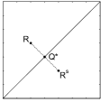
Figure 1: A point $R$, its swapped point $R^{S}$, the optimal approximation of both $Q^{*}$.

Preliminarily, as shown in Figure 1, we simply observe that if we consider in the Cartesian plane a point $R=(R_{x},R_{y})$, its optimal approximation $Q^{*}$, among the points $Q=(Q_{x},Q_{y})$ such that $Q_{x}=Q_{y}$, is obtained as the intersection between the line $y=x$, with the perpendicular line that pass through $R$, that is

$$\left\{\begin{array}[]{l}y-R_{y}=-(x-R_{x})\\ y=x\end{array}\right.$$

hence $Q_{x}^{*}=Q_{y}^{*}=\left(R_{x}+R_{y}\right)/2$. The same holds true if we consider the swapped point $R^{S}=(R_{y},R_{x})$, since they share the same distance, i.e., $d(R,Q^{*})=d(R^{S},Q^{*})$.

Clearly, due to linearity of obtained expression, this result can be extended also in the case of any linear combination of coordinates. Thus, by explicitly exploiting the structure of $A$ and $P$, we define as x-coordinate of a point the entry with negative index and as y-coordinate of the same point the corresponding entry with positive index. For the sake of simplicity we report an example for $q=3$, in which we put in evidence the x or y coordinate definition,

$$C = A-P=\left[\begin{array}[]{ccccccc}\omega_{0}^{y}&\nu_{1}^{x}&\nu_{2}^{x}&\nu_{3}^{x}&&&\\ \omega_{1}^{y}&\zeta_{0}^{y}&\zeta_{2}^{x}&\theta_{2}^{x}&\theta_{3}^{x}&&\\ \omega_{2}^{y}&\zeta_{1}^{y}&\theta_{0}&\theta_{1}^{x}&\theta_{2}^{x}&\theta_{3}^{x}&\\ \omega_{3}^{y}&\theta_{2}^{y}&\theta_{1}^{y}&\theta_{0}&\theta_{1}^{x}&\theta_{2}^{x}&\omega_{3}^{x}\\ &\theta_{3}^{y}&\theta_{2}^{y}&\theta_{1}^{y}&\theta_{0}&\zeta_{1}^{x}&\omega_{2}^{x}\\ &&\theta_{3}^{y}&\theta_{2}^{y}&\zeta_{2}^{y}&\zeta_{0}^{x}&\omega_{1}^{x}\\ &&&\nu_{3}^{y}&\nu_{2}^{y}&\nu_{1}^{y}&\omega_{0}^{x}\end{array}\right]-\left[\begin{array}[]{ccccccc}\hat{\omega}_{0}^{y}&0&0&0&&&\\ \hat{\omega}_{1}^{y}&\hat{\zeta}_{0}^{y}&\hat{\zeta}_{2}^{x}&\hat{\theta}_{2}^{x}&\hat{\theta}_{3}^{x}&&\\ \hat{\omega}_{2}^{y}&\hat{\zeta}_{1}^{y}&\hat{\theta}_{0}&\hat{\theta}_{1}^{x}&\hat{\theta}_{2}^{x}&\hat{\theta}_{3}^{x}&\\ \hat{\omega}_{3}^{y}&\hat{\theta}_{2}^{y}&\hat{\theta}_{1}^{y}&\hat{\theta}_{0}&\hat{\theta}_{1}^{x}&\hat{\theta}_{2}^{x}&\hat{\omega}_{3}^{x}\\ &\hat{\theta}_{3}^{y}&\hat{\theta}_{2}^{y}&\hat{\theta}_{1}^{y}&\hat{\theta}_{0}&\hat{\zeta}_{1}^{x}&\hat{\omega}_{2}^{x}\\ &&\hat{\theta}_{3}^{y}&\hat{\theta}_{2}^{y}&\hat{\zeta}_{2}^{y}&\hat{\zeta}_{0}^{x}&\hat{\omega}_{1}^{x}\\ &&&0&0&0&\hat{\omega}_{0}^{x}\end{array}\right]\text{,}$$

Here, we set the points

$$\Theta_{i} = (\theta_{i}^{x},\theta_{i}^{y})=(h_{-i},h_{i})$$

$$\Omega_{i} = (\omega_{i}^{x},\omega_{i}^{y})=(h_{-i}+2\sum_{j=i+1}^{q}h_{-j},h_{i}+2\sum_{j=i+1}^{q}h_{j})=(\theta_{i}^{x}+2\sum_{j=i+1}^{q}\theta_{j}^{x},\theta_{i}^{y}+2\sum_{j=i+1}^{q}\theta_{j}^{y})$$

$$N_{i} = (\nu_{i}^{x},\nu_{i}^{y})=(h_{-i}-h_{i},h_{i}-h_{-i})=(\theta_{i}^{x}-\theta_{i}^{Sx},\theta_{i}^{y}-\theta_{i}^{Sy})$$

and

$$Z_{0} = (\zeta_{0}^{x},\zeta_{0}^{y})=(h_{0}-h_{-2},h_{0}-h_{2})=(\theta_{0}^{x}-\theta_{2}^{x},\theta_{0}^{y}-\theta_{2}^{y})$$

$$Z_{1} = (\zeta_{1}^{x},\zeta_{1}^{y})=(h_{-1}-h_{-3},h_{1}-h_{3})=(\theta_{1}^{x}-\theta_{3}^{x},\theta_{1}^{y}-\theta_{3}^{y})$$

$$Z_{2} = (\zeta_{2}^{x},\zeta_{2}^{y})=(h_{-1}-h_{3},h_{1}-h_{-3})=(\theta_{1}^{x}-\theta_{3}^{Sx},\theta_{1}^{y}-\theta_{3}^{Sy})$$

related to the Hankel corrections. The points $\hat{\Theta}_{i}$, $\hat{\Omega}_{i}$, $\hat{Z}_{i}$ related to the matrix $P$ are defined in a similar manner, taking into account the strong symmetry property, i.e. they have the same x and y coordinates. More in general, the key idea is to transform the original minimization problem in the equivalent problem of minimizing the quantity

$$\begin{array}[]{l}c_{0}\mathbf{d}(\Theta_{0},\hat{\Theta}_{0})^{2}+\ldots+c_{q}\mathbf{d}(\Theta_{q},\hat{\Theta}_{q})^{2}+\mathbf{d}(Z_{0},\hat{Z}_{0})^{2}+\ldots+\mathbf{d}(Z_{m},\hat{Z}_{m})^{2}\\ \quad+\mathbf{d}(\Omega_{0},\hat{\Omega}_{0})^{2}+\ldots+\mathbf{d}(\Omega_{q},\hat{\Omega}_{q})^{2}+\mathbf{d}(N_{1},0)^{2}+\ldots+\mathbf{d}(N_{q},0)^{2},\end{array}$$ (19)

where $c_{j}$ are some constants taking into account the number of constant Toeplitz entries. Now, by referring to the initial geometrical observation, we start from points pertaining to the Toeplitz part, that can be minimized separately, and we obtain the minimizer (17). It is also an easy check to prove the same claim with respect to any other terms, by invoking the quoted linearity argument.

3.2 Two-dimensional case

Let $h_{PSF}=\left[h_{i_{1},i_{2}}\right]_{i_{1}=-q_{1},\ldots,q_{1},i_{2}=-q_{2},\ldots,q_{2}}$ be a generic PSF. As introduced in Section 2.2, the idea is to apply an anti-reflection with respect to the border points $f_{1,i_{2}}$, $f_{i_{1},1}$ and $f_{n_{1},i_{2}}$, $f_{i_{1},n_{2}}$, $i_{1}=1,\ldots,n_{1}$, $i_{2}=1,\ldots,n_{2}$, and a double anti-reflection at the corners in order to preserve the tensorial structure. The resulting matrix shows a more involved structure, i.e., it is block Toeplitz + Hankel with Toeplitz + Hankel blocks plus a structured low rank correction matrix, as follows

V1⋮Vq1BWq1⋮W10−JUW0]​,𝐴delimited-[]fragments fragmentsV1missing-subexpressionmissing-subexpressionmissing-subexpressionmissing-subexpressionmissing-subexpressionmissing-subexpression⋮missing-subexpressionmissing-subexpressionmissing-subexpressionmissing-subexpressionmissing-subexpressionmissing-subexpressionfragmentsVsubscript𝑞1missing-subexpressionmissing-subexpression𝐵missing-subexpressionmissing-subexpressionfragmentsWsubscript𝑞1missing-subexpressionmissing-subexpressionmissing-subexpressionmissing-subexpressionmissing-subexpressionmissing-subexpression⋮missing-subexpressionmissing-subexpressionmissing-subexpressionmissing-subexpressionmissing-subexpressionmissing-subexpressionfragmentsW10fragmentsJUfragmentsW0,A=\left[\begin{tabular}[]{c|ccccc|c}$V_{0}$&\vrule\lx@intercol\hfil$U$\hfil\lx@intercol\vrule\lx@intercol &$0$\\ \hline\cr$V_{1}$&&&&&&\\ $\vdots$&&&&&&\\ $V_{q_{1}}$&&&$B$&&&$W_{q_{1}}$\\ &&&&&&$\vdots$\\ &&&&&&$W_{1}$\\ \hline\cr$0$&\vrule\lx@intercol\hfil$-JU$\hfil\lx@intercol\vrule\lx@intercol &$W_{0}$\end{tabular}\right]\text{,}

V0U0V0U0 (20)

with

$$U = \left[\hat{H}_{-1}-\hat{H}_{1},\ldots,\hat{H}_{-q_{1}}-\hat{H}_{q_{1}},0,\ldots,0\right]\text{,}\ -JU=\left[0,\ldots,0,\hat{H}_{q_{1}}-\hat{H}_{-q_{1}},\ldots,\hat{H}_{1}-\hat{H}_{-1}\right]\text{,}$$

$$V_{j} = \hat{H}_{j}+2\underset{i=j+1}{\overset{q_{1}}{\sum}}\hat{H}_{i}\text{,}\quad W_{j}=\hat{H}_{-j}+2\underset{i=j+1}{\overset{q_{1}}{\sum}}\hat{H}_{-i}\text{,}$$

$$B = T(\hat{H}_{-q_{1}},\ldots,\hat{H}_{q_{1}})-H_{\mathrm{TL}}(\hat{H}_{2},\ldots,\hat{H}_{q_{1}})-H_{\mathrm{BR}}(\hat{H}_{-2},\ldots,\hat{H}_{-q_{1}})\text{.}$$

where $T$ indicates the block Toeplitz matrix, while $H_{\mathrm{TL}}$ and $H_{\mathrm{BR}}$ are respectively the top-left block Hankel matrix and the bottom-right block Hankel matrix as just previously depicted in the unilevel setting and where the block $\hat{H}_{j}$ is defined, according to (15), as

vj,1⋮vj,q2Bjwj,q2⋮wj,10−(Juj)Twj,0]​,subscript^𝐻𝑗delimited-[]fragments fragmentsv𝑗1missing-subexpressionmissing-subexpressionmissing-subexpressionmissing-subexpressionmissing-subexpressionmissing-subexpression⋮missing-subexpressionmissing-subexpressionmissing-subexpressionmissing-subexpressionmissing-subexpressionmissing-subexpressionfragmentsv𝑗subscript𝑞2missing-subexpressionmissing-subexpressionfragmentsB𝑗missing-subexpressionmissing-subexpressionfragmentsw𝑗subscript𝑞2missing-subexpressionmissing-subexpressionmissing-subexpressionmissing-subexpressionmissing-subexpressionmissing-subexpression⋮missing-subexpressionmissing-subexpressionmissing-subexpressionmissing-subexpressionmissing-subexpressionmissing-subexpressionfragmentsw𝑗10fragments(Ju𝑗)𝑇fragmentsw𝑗0,\hat{H}_{j}=\left[\begin{tabular}[]{c|ccccc|c}$v_{j,0}$&\vrule\lx@intercol\hfil$u_{j}^{T}$\hfil\lx@intercol\vrule\lx@intercol &$0$\\ \hline\cr$v_{j,1}$&&&&&&\\ $\vdots$&&&&&&\\ $v_{j,q_{2}}$&&&$B_{j}$&&&$w_{j,q_{2}}$\\ &&&&&&$\vdots$\\ &&&&&&$w_{j,1}$\\ \hline\cr$0$&\vrule\lx@intercol\hfil$-(Ju_{j})^{T}$\hfil\lx@intercol\vrule\lx@intercol &$w_{j,0}$\end{tabular}\right]\text{,}

vj,0ujT0vj,0ujT0 (21)

with $B_{j}=T(h_{j,-q_{2}},\ldots,h_{j,q_{2}})-H_{\mathrm{TL}}(h_{j,2},\ldots,h_{j,q_{2}})-H_{\mathrm{BR}}(h_{j,-2},\ldots,h_{j,-q_{2}})$.

Refer to (10) and (11) for the structure of the matrix $P$ related to a strongly symmetric PSF in which the minimizer $P^{*}$, see (13), will be searched.

Theorem 3.2

Let $A=A(h)$ be the Anti-Reflective matrix generated by the generic PSF $h_{PSF}=\left[h_{i_{1},i_{2}}\right]_{i_{1}=-q_{1},\ldots,q_{1},i_{2}=-q_{2},\ldots,q_{2}}$.
The optimal preconditioner in the $\mathcal{AR}_{n}^{2D}$ algebra is the matrix associated with the symmetrized PSF $s_{PSF}=\left[s_{i_{1},i_{2}}\right]_{i_{1}=-q_{1},\ldots,q_{1},i_{2}=-q_{2},\ldots,q_{2}}$, with

$$s_{\pm i_{1},\pm i_{2}}=\dfrac{h_{-i_{1},-i_{2}}+h_{-i_{1},i_{2}}+h_{i_{1},-i_{2}}+h_{i_{1},i_{2}}}{4}\text{.}$$ (22)

Proof

The proof can be done by extending the geometrical approach just considered in the one-dimensional case: we simply observe that if we consider in the $4$-dimensional space a point $R=(R_{x},R_{y},R_{z},R_{w})$, its optimal approximation $Q^{*}$ among the points $Q=(Q_{x},Q_{y},Q_{z},Q_{w})$ belonging to the line $\mathcal{L}$

$$\left\{\begin{array}[]{c}x=t\\ y=t\\ z=t\\ w=t\end{array}\right.$$

is obtained by minimizing the distance

$$\mathbf{d}^{2}(\mathcal{L},R) = 4t^{2}-2t(R_{x}+R_{y}+R_{z}+R_{w})+R_{x}^{2}+R_{y}^{2}+R_{z}^{2}+R_{w}^{2}\text{.}$$

This is a trinomial of the form $\alpha t^{2}+\beta t+\gamma$, with $\alpha>0$ and we find the minimum by using the formula for computing the abscissa of the vertex of a parabola

$${t}^{*}=-\frac{\beta}{2\alpha}=\frac{R_{x}+R_{y}+R_{z}+R_{w}}{4}\text{.}$$

Hence the point $Q^{*}$ is defined as $Q^{*}_{x}=Q^{*}_{y}=Q^{*}_{z}=Q^{*}_{w}=t^{*}$. The same holds true if we consider any swapped point $R^{S}$, not unique but depending on the permutation at hand, since they share the same distance, i.e., $d(R,Q^{*})=d(R^{S},Q^{*})$. Again, thanks to the linearity of obtained expression, this result can be extended also in the case of any linear combination of coordinates.

Thus, by explicitly exploiting the structure of the matrices $A$ and $P$, we define a point by referring to the entry with positive and negative two-index. For instance, points pertaining to the Toeplitz part are defined as

$$\Theta_{i_{1},i_{2}} = (\theta_{i_{1},i_{2}}^{x},\theta_{i_{1},i_{2}}^{y},\theta_{i_{1},i_{2}}^{z},\theta_{i_{1},i_{2}}^{w})=(h_{-i_{1},-i_{2}},h_{-i_{1},i_{2}},h_{i_{1},-i_{2}},h_{i_{1},i_{2}}),$$

$$\hat{\Theta}_{i_{1},i_{2}} = (\hat{\theta}_{i_{1},i_{2}}^{x},\hat{\theta}_{i_{1},i_{2}}^{y},\hat{\theta}_{i_{1},i_{2}}^{z},\hat{\theta}_{i_{1},i_{2}}^{w})=(s_{-i_{1},-i_{2}},s_{-i_{1},i_{2}},s_{i_{1},-i_{2}},s_{i_{1},i_{2}}),$$

respectively.

As in the unilevel setting, the original minimization problem is transformed in the equivalent problem of minimizing the sum of squared distances analogously as in (19). We start again from points pertaining to the Toeplitz part, that can be minimized separately, and we obtain the minimizer (22). It is also an easy check to prove the same claim with respect to any other couple of points pertaining to Hankel or low rank corrections, by invoking the quoted linearity argument.

It is worth stressing that this proof idea is very powerful in its generality. It can be applied to any type of BCs based on the fact that the values of unknowns outside the FOV are defined as linear combinations of the unknowns inside the FOV, so that it may be useful in the future to prove theoretical results for new proposed BCs.

4 Computational results

A well-known iterative method for solving the image deblurring problem is Landweber method Landweber , whose $(k+1)$-th iteration step is defined by

$$x_{k+1}=x_{k}+\tau A^{H}(g-Ax_{k}),$$ (23)

where $A$ is the blurring matrix, $g$ is the recorded image and $\tau$ is the descent parameter (we set it equal to one). As one can observe experimentally, the restorations seem to converge in the initial iterations, before they become worse and finally diverge; this phenomenon is called semiconvergence. Hence Landweber method is a regularization method, where the number of steps $k$ is the regularization parameter. Moreover it has good stability properties, but it is usually very slow to converge to the sought solution. Therefore it is a good candidate for testing the proposed preconditioning technique. Thus we introduce the preconditioned Landweber method

$$x_{k+1}=x_{k}+\tau DA^{H}(g-Ax_{k}),$$ (24)

where $D$ is the preconditioner. In order to build it, we compute the eigenvalues $\lambda_{j}$ of the blurring matrix associated to the PSF and to periodic BCs (via FFT) or to the symmetrized PSF and to Reflective BCs (via FCT) or to the symmetrized PSF and to Anti-Reflective BCs (via FST, see Theorem 2.1 and Theorem 2.2 and comments below), then we apply the Tikhonov Filter

$$\begin{array}[]{cc}d_{j}=\dfrac{1}{\left|\lambda_{j}\right|^{2}+\alpha}\end{array}$$ (25)

to determine the eigenvalues $d_{j}$ of $D$; finally the PSF related to $D$ can be obtained via IFFT or IFCT or IFST (the inverses of the previous transforms, namely inverse FFT, inverse FCT, inverse FST)). In numerical experiments we have set the parameter $\alpha$ manually, so that we have reached excellent performances both in terms of quality of the restorations and in acceleration of the method.

Actually in our implementation, which is partially based on the Matlab Toolbox RestoreTools NagyTools , we have never worked with $A^{H}$, but always with $A^{\prime}$, that is the matrix related to the PSF rotated by 180 degrees. This approach is known in literature as reblurring strategy DS-IP-2005 . The reason behind this choice resides in one of the main problems of Anti-Reflective algebra $\mathcal{AR}$, i.e. the fact that it is not closed under transposition. We stress that $A^{H}$ and $A^{\prime}$ are the same thing in case of periodic and zero boundary conditions, but they are different for Reflective and Anti-Reflective ones.

To test these different BCs and preconditioning techniques, we have taken into account the Cameraman deblurring problem of Figure 2, in which the PSF is a slightly non-symmetric portion of a Gaussian blur, and the Bridge deblurring problem of Figure 5, in which the PSF is an highly non-symmetric portion of a Gaussian blur. In both cases we have generated the blurred and noisy data $g$, adding about $0.1\%$ of white Gaussian noise. We have chosen to add a low level of noise to emphasize the importance of boundary conditions, which play a leading role when the noise is low, while they become less decisive when it grows up. Since we know the true image $f$, to measure the quality of the deblurred images we compute the Relative Restoration Error (RRE) $\left\|x-f\right\|_{\cal F}/\left\|f\right\|_{\cal F}$, where $\left\|\cdot\right\|_{\cal F}$ is the Frobenius norm and $x$ is the computed restoration.

As we expected, from Table 1 and Table 2, we can notice that both Reflective and Anti-Reflective boundary conditions outperform periodic ones, which give rise to poor restorations (see first image of Figure 3 and Figure 6). Furthermore by means of Anti-Reflective BCs (see third image of Figure 3 and Figure 6) we can gain restorations of better quality compared with ones obtained employing Reflective BCs (see second image of Figure 3 and Figure 6). From Tables 1-2 and Figures 4-7 we can see that all these considerations hold also for $D$-Landweber method — i.e. Landweber method with preconditioning — which for a suitable choice of the parameter $\alpha$ is able to reach restorations of the same quality of the classical Landweber method in much smaller number of steps. In particular the reduction in steps for both Reflective and Anti-Reflective BCs is around $50$ times for the Cameraman deblurring problem and around $8$ for the Bridge deblurring problem.

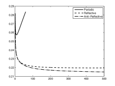
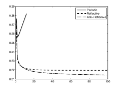
We stress that the iteration count reported in Table 2 in the Anti-Reflective row does not have to deceive, because, as it can be seen from Figure 8, if we compare the restorations gained by Landweber (preconditioned or not) at any given fixed iteration, employing Reflective BCs or Anti-Reflective BCs, we see that the latter shows always equal or better restoration quality. The same remark holds for the Cameraman deblurring problem (see Table 1). In fact Figure 8 is very instructive because it tells to the generic user two things: a) the curves for Reflective and Anti-Reflective BCs are very flat, b) the approximation obtained when using Anti-Reflective BCs is always better or equal to that obtained with Reflective BCs. The combined message of the previous two items is that we can safely choose the Anti-Reflective BCs, even when we are unable to estimate precisely the stopping criterion for deciding the optimal iteration: we notice that this observation does not hold for the periodic BCs where a small error in the evaluation of the optimal iteration leads to a substantial deterioration of the quality of the resulting restored image.

In the end, from the results reported in this section we can say that our proposal of the optimal preconditioner in the context of Anti-Reflective BCs is as effective as the one introduced in NCT-SISC-1999 for Reflective BCs. Therefore the present work represents a theoretical and numerical continuation and strengthening of that line of research.

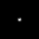
Figure 2: Cameraman deblurring problem: true image, PSF, blurred and noisy image.

	Landweber		$D$-Landweber
	RRE	IT	RRE	IT
Periodic	0.2147	46	0.2136	3
Reflective	0.1611	953	0.1611	19
Anti-Reflective	0.1582	1461	0.1582	25

Table 1: Results of the classical and preconditioned Landweber method related to the Cameraman deblurring problem, employing different BCs.

Figure 3: Landweber restorations, employing periodic, reflective, anti-reflective BCs.

Figure 4: Preconditioned Landweber restorations, employing periodic, reflective, anti-reflective BCs.

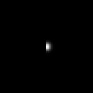
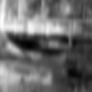
Figure 5: Bridge deblurring problem: true image, PSF, blurred and noisy image.

	Landweber		$D$-Landweber
	RRE	IT	RRE	IT
Periodic	0.2573	9	0.2561	2
Reflective	0.2195	1281	0.2195	146
Anti-Reflective	0.2114	12824	0.2114	1718

Table 2: Results of the classical and preconditioned Landweber method related to the Bridge deblurring problem, employing different BCs.

Figure 6: Landweber restorations, employing periodic, reflective, anti-reflective BCs.

Figure 7: Preconditioned Landweber restorations, employing periodic, reflective, anti-reflective BCs.

Figure 8: Bridge deblurring problem: RRE trends of Landweber (on the left) and $D$-Landweber (on the right) for different BCs.

5 Conclusions and Perspectives

Inspired by the theoretical results on optimal preconditioning stated in NCT-SISC-1999 in the Reflective BCs environment, in this paper we have presented analogous results for Anti-Reflective BCs. In both cases the optimal preconditioner is the blurring matrix associated to the symmetrized PSF. We stress that our proof is based on a geometrical idea, which allows to greatly simplify the used arguments, even when non orthogonal transforms are involved. Moreover that idea is very powerful in its generality and it may be useful in the future to prove theoretical results for new BCs.

Computational results have shown that the proposed preconditioning strategy is effective and it is able to give rise to a meaningful acceleration both for slightly and highly non-symmetric PSFs. On the other hand, symmetrization is efficient when we have a PSF that is near to be symmetric and it becomes more and more ineffective as the PSF departs from symmetry. In this case, other techniques Z2 , which can manage directly non-symmetric structures, can gain better performances and in this direction we see a substantial development in the near future.

References

• (1) A. Aricò, M. Donatelli, and S. Serra Capizzano, The Antireflective Algebra: Structural and Computational Analysis with Application to Image Deblurring and Denoising, Calcolo, 45–3 (2008), pp. 149–175.
• (2) A. Aricò, M. Donatelli, and S. Serra Capizzano, Spectral analysis of the anti-reflective algebra, Linear Algebra Appl., 428, 2-3 (2008), pp. 657–675.
• (3) A. Aricò, M. Donatelli, J. Nagy, and S. Serra Capizzano, The anti-reflective transform and regularization by filtering, special volume Numerical Linear Algebra in Signals, Systems, and Control., in Lecture Notes in Electrical Engineering, Springer Verlag., Vol. 80 (2011) pp. 1–21.
• (4) M. Bertero, P. Boccacci. Introduction to inverse problems in imaging. Institute of Physics Publ., Bristol (1998).
• (5) D. Bini and M. Capovani, Spectral and computational properties of band symmetric Toeplitz matrices, Linear Algebra Appl., 52/53 (1983), pp. 99–126.
• (6) P. J. Davis, Circulant Matrices, Wiley, New York (1979).
• (7) P. Dell’Acqua, M. Donatelli, C. Estatico. A general Z variant for iterative and direct regularization methods, in preparation.
• (8) M. Donatelli, C. Estatico, J. Nagy, L. Perrone, and S. Serra Capizzano, Anti-reflective boundary conditions and fast 2D deblurring models, Proceeding to SPIE’s 48th Annual Meeting, San Diego, CA USA, F. Luk Ed, 5205 (2003), pp. 380–389.
• (9) M. Donatelli, C. Estatico, A. Martinelli, and S. Serra Capizzano, Improved image deblurring with anti-reflective boundary conditions and re-blurring, Inverse Problems, 22 (2006), pp. 2035–2053.
• (10) M. Donatelli and S. Serra Capizzano, Anti-reflective boundary conditions and re-blurring, Inverse Problems, 21 (2005), pp. 169–182.
• (11) H. W. Engl, M. Hanke, A. Neubauer. Regularization of inverse problems. Mathematics and its Applications, 375. Kluwer Academic Publishers, Dordrecht (1996).
• (12) P. C. Hansen. Rank-deficient and discrete ill-posed problems. SIAM, Philadelphia (1998).
• (13) P. C. Hansen, J. G. Nagy, D. P. OLeary. Deblurring images: matrices, spectra and filtering. SIAM, Philadelphia (2006).
• (14) R. L. Lagendijk and J. Biemond, Iterative Identification and Restoration of Images, Springer-Verlag, New York (1991).
• (15) L. Landweber. An iteration formula for Fredholm integral equations of the first kind. Amer. J. Math. 73 (1951), pp. 615-624.
• (16) J. G. Nagy, K. Palmer, L. Perrone Iterative Methods for Image Deblurring: A Matlab Object Oriented Approach. Numer. Algorithms, 36 (2004), pp. 73–93.
• (17) M. K. Ng, R. H. Chan, and W. C. Tang, A fast algorithm for deblurring models with Neumann boundary conditions, SIAM J. Sci. Comput., 21-3 (1999), pp. 851–866.
• (18) L. Perrone, Kronecker Product Approximations for Image Restoration with Anti-Reflective Boundary Conditions, Numer. Linear Algebra Appl., 13–1 (2006), pp. 1–22.
• (19) Y. Shi and Q. Chang, Acceleration methods for image restoration problem with different boundary conditions, Applied Numerical Mathematics, 58-5 (2008), pp. 602 -614.
• (20) S. Serra Capizzano, A note on anti-reflective boundary conditions and fast deblurring models, SIAM J. Sci. Comput., 25–3 (2003), pp. 1307–1325.
• (21) G. Strang, The Discrete Cosine Transform, SIAM Review, 41–1 (1999), pp. 135–147.
• (22) C. Tablino Possio, Truncated decompositions and filtering methods with Reflective/Anti-Reflective boundary conditions: a comparison, in Matrix methods: theory, algorithms, applications. Dedicated to the Memory of Gene Golub, V. Olshevsky, E. Tyrtyshnikov Eds., World Scientific Publishing (2010), pp. 382-408.