Supersymmetric type-III seesaw:
lepton flavour violation and LHC phenomenology

Abstract

We study a supersymmetric version of the seesaw mechanism type-III considering two variants of the model: a minimal version for explaining neutrino data with only two copies of ${\bf 24}$ superfields and a model with three generations of ${\bf 24}$-plets. The latter predicts in general rates for $\mu\to e\gamma$ inconsistent with experimental data. However, this bound can be evaded if certain special conditions within the neutrino sector are fulfilled. In case of two ${\bf 24}$-plets lepton flavour violation constraints can be satisfied much easier. After specifying the corresponding regions in the mSugra parameter space we show that under favorable conditions one can test the corresponding flavour structures in the leptonic sector at the LHC. For this we perform Monte Carlo studies for the signals taking also into account the SUSY background. We find that it is only of minor importance for the scenarios studied here.

I Introduction

Neutrino oscillation experiments give currently the main indication for physics beyond the Standard Model (SM). The observed tiny neutrino masses can be easily explained by the seesaw mechanism, which at tree level can be written in just three different variants Ma:1998dn , classified according to the $SU(2)\times U(1)$ representation of the postulated heavy particles: type I postulates fermionic gauge singlets Minkowski:1977sc ; Yanagida:1979as ; GellMann:1980vs ; Mohapatra:1979ia , type II scalar $SU(2)$-triplets with hypercharge 1 Schechter:1980gr ; Cheng:1980qt and type III fermionic triplets in the adjoint representation of $SU(2)$ Foot:1988aq . At low energies they all lead to a unique dimension-5 operator Weinberg:1979sa ; Weinberg:1980bf

$$(m^{\nu})_{\alpha\beta}=\frac{f_{\alpha\beta}}{\Lambda}(HL)(HL).$$ (1)

Neutrino experiments determine only $f_{\alpha\beta}/\Lambda$, but contain no information about the origin of this operator, nor about the absolute size of $\Lambda$. If $f$ is a coefficient ${\cal O}(1)$, current neutrino data indicates $\Lambda\raise 1.29167pt\hbox{$\;<$\kern-7.5pt\raise-4.73611pt\hbox{$\sim\;$}}{\cal O}(10^{15})$ GeV. This value is close to, but slightly below the scale of hypothetical great unified theory (GUT) which should be larger than roughly $10^{16}$ GeV to avoid bounds from the non-observation of proton decay.

A possible way to stabilise the large hierarchy between the GUT scale and the electroweak scale is supersymmetry Witten:1981nf . In its minimal form it leads to an unification of the gauge couplings in contrast to the SM Dimopoulos:1981yj ; Ibanez:1981yh ; Marciano:1981un ; Einhorn:1981sx ; Amaldi:1991cn ; Langacker:1991an ; Ellis:1990wk . Moreover it can explain electroweak symmetry breaking as a radiative effect Ibanez:1982fr . Supersymmetric variants of the different seesaw models have been considered by several authors, see e.g. Hisano:1998wn ; Rossi:2002zb ; Buckley:2006nv ; Hirsch:2008gh ; Borzumati:2009hu ; Esteves:2010ff . In these models renormalisation group evolution induce non-zero flavour mixing elements in the mass parameters of the sleptons even if they are flavour diagonal at the GUT scale. These in turn leads to sizeable contributions to lepton flavour violating (LFV) observables Borzumati:1986qx . In case of seesaw type-I, low energy LFV decays such as $l_{i}\to l_{j}+\gamma$ and $l_{i}\to 3l_{j}$ have been calculated in Hisano:1995nq ; Hisano:1995cp ; Ellis:2002fe ; Deppisch:2002vz ; Petcov:2003zb ; Arganda:2005ji ; Petcov:2005yh ; Antusch:2006vw ; Deppisch:2004fa ; Hirsch:2008dy ; $\mu-e$ conversion in nuclei has been studied in Arganda:2007jw ; Deppisch:2005zm .

To maintain gauge coupling unification the seesaw particles need to be included in complete $SU(5)$ representations, i.e. one needs a 15-plet in case of type II and at least two 24-plets in case of type III models. If one were to use only one 24-plet, then one would need either non-renormalizable operators at the GUT-scale Biggio:2010me or an extended $SU(5)$ Higgs sector Perez:2007iw to explain neutrino data. The type-II and type-III models have received less attention than type-I. Note, however, that the former has actually fewer free parameters than type-I implying that ratios of LFV decays of leptons can actually be predicted as a function of neutrino angles in minimal supergravity (mSUGRA) as discussed in Rossi:2002zb ; Hirsch:2008gh . For type-III it has been shown in ref. Esteves:2010ff that a generic model with three 24-plets is heavily constrained by the bounds on rare lepton decays, in particular due to the stringent bound on $\mu\to e\gamma$. The impact on $\mu\to e\gamma$ in a gauge mediated supersymmetry breaking (GMSB) embedding of type-III was studied in ref. Mohapatra:2008wx , while in ref. Abada:2011mg also possible LHC phenomenology from lepton-flavor violation has been discussed for the mSUGRA case.

In this paper we are first going to show under which conditions the type-III model is consistent with the experimental data. This will then be compared with a two generation model where the bounds due to $\mu\to e\gamma$ are less stringent. Finally we will address the question to which extent LHC might observe lepton flavour violating processes in supersymmetric (SUSY) cascade decays. Compared to the previous study in ref. Abada:2011mg we do not only consider the case of two as well as of three generations of 24-plets, but we also take into account the recently measured reactor angle $\theta_{13}$. Moreover, we demonstrate in a Monte Carlo study for the LHC signal that the SUSY background is well under control.

For the particle content we will assume the MSSM as framework. The recent observation of a Higgs like state at the LHC with a mass around 125 GeV ATLAS:2012ae ; Chatrchyan:2012tx can hardly be explained within GUT models with universal boundary conditions Bechtle:2012zk ; Buchmueller:2012hv . The same holds in variants including seesaw states at high scales Hirsch:2012ti . However, it is well-known that singlet extension of the MSSM can more easily explain a Higgs mass of this size as there are additional F-term contributions already at tree-level, see e.g. Ellwanger:2012ke ; Gunion:2012zd ; Ross:2011xv and references therein. Including an additional singlet does not lead to any significant changes in the slepton sector as the singlet Yukawa couplings enter only at two-loop level in the RGEs of the corresponding parameters. For this reason we do consider bounds from direct searches at the LHC but do not take into account the requirement of correctly explaining a Higgs mass of 125 GeV. To explain also this condition and taking into account the theoretical as well experimental uncertainty it would be sufficient to shift the tree-level Higgs mass for all points in the following by about 5 GeV. In the next-to minimal supersymmetric standard model (NMSSM) the tree-level mass of the light Higgs is given by Ellwanger:2009dp .

$$m^{2}_{Z}\left(\cos^{2}2\beta+\frac{\lambda^{2}}{g^{2}}sin^{2}2\beta\right)$$ (2)

where we introduced the superpotential coupling $\lambda$ of the singlet to the Higgs doublets. Thus, assuming $\tan\beta=10$ one would need $\lambda\simeq 0.6$, i.e. not too close to the perturbativity bound of 0.75. However, the exact value of $\tan\beta$ plays only a sub-dominant role for our analysis in the following. If we choose $\tan\beta=5$, already $\lambda=0.45$ would be sufficient. Since the singlino couples only very weakly to the sleptons its role is negligible as long as it isn’t the LSP. However, it can only be the LSP if the trilinear self coupling $\kappa$ of the singlet field is much smaller than $\lambda$ Choi:2004zx . For example in the scale invariant NMSSM a bino LSP is a common feature Cheung:2012qy . Moreover, this constraint can easily be satisfied in more general singlet extensions with an explicit bilinear singlet term in the superpotential Delgado:2012yd ; Ross:2012nr .

This paper is organised as follows: in the next section we summarise the main features of the two variants of the type-III model. In section III we first discuss how to accommodate the rare lepton decays in type III seesaw models. Afterwards we discuss lepton flavour violating signals from SUSY cascade decays and present the results of a Monte Carlo study. Finally we draw in section IV our conclusions.

II Models and spectra

In this section we briefly summarise the main features of the supersymmetric version of the seesaw type-III model. In order to maintain gauge coupling unification for type-III we add at the seesaw scale(s) additional particles to obtain complete $SU(5)$ representation, i.e. a 24-plet. Note that the 24-plet actually also includes a gauge singlet and, thus, one has always a combination of the type I and the type III seesaw in this model.

In the subsequent sections we present the superpotentials and the relation of the parameters to neutrino physics. In addition, there are the corresponding soft SUSY breaking terms which, however, reduce at the electro-weak scale to the MSSM ones and, thus, are not discussed further. There are additional terms of the soft SUSY breaking potential, due to the heavy particles, that we do not discuss either, as their effect is at most of the order $M_{EWSB}/M_{seesaw}$ and, thus, can be safely neglected.

In this paper we will assume common soft SUSY breaking parameters at the GUT-scale $M_{GUT}$ to specify the spectrum at the electro-weak scale: a common universal gaugino mass $M_{1/2}$, a common scalar mass $m_{0}$ and the trilinear coupling $A_{0}$ which gets multiplied by the corresponding Yukawa couplings to obtain the trilinear couplings in the soft SUSY breaking Lagrangian. In addition the sign of the $\mu$ parameter is fixed, as is $\tan\beta=v_{u}/v_{d}$ (at the electro-weak scale), where $v_{d}$ and $v_{u}$ are the the vacuum expectation values (vevs) of the neutral component of $H_{d}$ and $H_{u}$, respectively. The models discussed below also contain new bilinear parameters in the superpotential leading to additional bilinear terms in the soft SUSY breaking potential which are proportional to $B_{0}$ of the MSSM Higgs sector. The corresponding RGEs decouple and their only effect is a small mass splitting between the new heavy scalar particles from the new heavy fermionic states of the order $B_{0}/M_{seesaw}$. This leads to a tiny effect in the calculation of the thresholds at the seesaw scale(s) Kang:2010zd which, however, we can safely neglect.

II.1 Supersymmetric seesaw type-III

In the case of a seesaw model type-III one needs new fermions $\Sigma$ at the high scale belonging to the adjoint representation of $SU(2)$. This has to be embedded in a 24-plet to obtain a complete $SU(5)$ representation. The superpotential of the unbroken $SU(5)$ relevant for our discussion is

$$W = \sqrt{2}\,{\bar{5}}_{M}Y^{5}10_{M}{\bar{5}}_{H}-\frac{1}{4}10_{M}Y^{10}10_{M}5_{H}+5_{H}24_{M}Y^{III}_{N}{\bar{5}}_{M}+\frac{1}{2}24_{M}M_{24}24_{M}\thickspace.$$ (3)

Here we have not specified the Higgs sector responsible for the $SU(5)$ breaking as it only enters logarithmically via threshold corrections at the GUT-scale and, thus, plays a minor rôle for the subsequent discussion. The new parts, which will give the seesaw mechanism, come from the $24_{M}$. It decomposes under $SU(3)\times SU(2)\times U(1)$ as

$$24_{M} = (1,1,0)+(8,1,0)+(1,3,0)+(3,2,-5/6)+(3^{*},2,5/6)\thickspace,$$

$$= \widehat{B}_{M}+\widehat{G}_{M}+\widehat{W}_{M}+\widehat{X}_{M}+\widehat{\bar{X}}_{M}\thickspace.$$

The fermionic components of $(1,1,0)$ and $(1,3,0)$ have exactly the same quantum numbers as a right-handed neutrino $\nu^{c}$ and the required $SU(2)$-triplet $\Sigma$. Thus, the $24_{M}$ always produces a combination of the type-I and type-III seesaws.

In the $SU(5)$ broken phase the superpotential becomes

$$W_{III} = W_{MSSM}+\widehat{H}_{u}(\widehat{W}_{M}Y_{N}-\sqrt{\frac{3}{10}}\widehat{B}_{M}Y_{B})\widehat{L}+\widehat{H}_{u}\widehat{\bar{X}}_{M}Y_{X}\widehat{D}^{c}$$ (5)

$$+\frac{1}{2}\widehat{B}_{M}M_{B}\widehat{B}_{M}+\frac{1}{2}\widehat{G}_{M}M_{G}\widehat{G}_{M}+\frac{1}{2}\widehat{W}_{M}M_{W}\widehat{W}_{M}+\widehat{X}_{M}M_{X}\widehat{\bar{X}}_{M}\,.s$$

As before we use at the GUT scale the boundary condition $Y_{N}=Y_{B}=Y_{X}$ and $M_{B}=M_{G}=M_{W}=M_{X}$. $Y_{N}$, $Y_{B}$ and $Y_{X}$ are $n\times 3$ while $M_{G}$, $M_{W}$ and $M_{X}$ are $n\times n$-dimensional matrices if we include $n$ generations of 24-plets. Integrating out the heavy fields yields the following formula for the neutrino masses at the low scale:

$$m_{\nu}=-\frac{v^{2}_{u}}{2}\left(\frac{3}{10}Y^{T}_{B}M^{-1}_{B}Y_{B}+\frac{1}{2}Y^{T}_{W}M^{-1}_{W}Y_{W}\right).$$ (6)

As mentioned above there are two contributions, one from the gauge singlet the other from the $SU(2)$ triplet. In this case the calculation of the Yukawa couplings in terms of a given high scale spectrum is more complicated than in the other two types of seesaw models. However, as we start from universal couplings and masses at $M_{GUT}$ we find that at the seesaw scale one still has $M_{B}\simeq M_{W}$ and $Y_{B}\simeq Y_{W}$ so that one can write in a good approximation

$$m_{\nu}=-v^{2}_{u}\frac{4}{10}Y^{T}_{W}M^{-1}_{W}Y_{W}\,.$$ (7)

Being complex symmetric, the light Majorana neutrino mass matrix in eq. (7), is diagonalized by a unitary $3\times 3$ matrix $U$ Schechter:1980gr

$${\hat{m}_{\nu}}=U^{T}\cdot m_{\nu}\cdot U\ .$$ (8)

Inverting the seesaw equation, eq. (7), allows to express $Y_{W}$ as Casas:2001sr

$$Y_{W}=\frac{i4\sqrt{2}}{5v_{u}}\sqrt{\widehat{W}_{M}}\cdot R\cdot\sqrt{{\hat{m}_{\nu}}}\cdot U^{\dagger},$$ (9)

for $n=3$ where the $\hat{m}_{\nu}$ and $\widehat{W}_{M}$ are diagonal matrices containing the corresponding eigenvalues. $R$ is in general a complex orthogonal matrix which is characterised by three angles $\phi_{i}$ which are in general complex. Note that, in the special case $R={\bf 1}$, $Y_{W}$ contains only “diagonal” products $\sqrt{M_{i}m_{i}}$. For $U$ we will use the standard form

$$U=\left(\begin{array}[]{ccc}c_{12}c_{13}&s_{12}c_{13}&s_{13}e^{-i\delta}\\ -s_{12}c_{23}-c_{12}s_{23}s_{13}e^{i\delta}&c_{12}c_{23}-s_{12}s_{23}s_{13}e^{i\delta}&s_{23}c_{13}\\ s_{12}s_{23}-c_{12}c_{23}s_{13}e^{i\delta}&-c_{12}s_{23}-s_{12}c_{23}s_{13}e^{i\delta}&c_{23}c_{13}\end{array}\right)\times\left(\begin{array}[]{ccc}e^{i\alpha_{1}/2}&0&0\\ 0&e^{i\alpha_{2}/2}&0\\ 0&0&1\end{array}\right)$$ (16)

with $c_{ij}=\cos(\theta_{ij})$ and $s_{ij}=\sin(\theta_{ij})$. The angles $\theta_{12}$, $\theta_{13}$ and $\theta_{23}$ are the solar neutrino angle, the reactor (or CHOOZ) angle and the atmospheric neutrino mixing angle, respectively. $\delta$ is the Dirac phase and $\alpha_{i}$ are Majorana phases. In the following we will set the latter to 0 and consider for $\delta$ mainly the cases $0$ and $\pi$.

II.2 Supersymmetric seesaw type-III with two 24-plets

Current neutrino experiments only determine the differences of the neutrino masses squared. Thus it might well be that only two of the light neutrinos are massive whereas the third is either massless or has a mass much smaller than the others. Such a situation is obtained if only two 24-plets are present similarly to the case of the seesaw type I with two right-handed neutrinos as discussed for example in ibarra2m24 ; 2m24b ; 2m24c . We call this class of models $3\times 2$ seesaw, see also masiero_vives .

In the following we work in the basis where $M_{W}$ is a $2\times 2$ diagonal matrix denoting the eigenvalues by $\hat{M}_{i}$ ($i=1,2$). Similarly to the three generation case one can express the $Y_{W}$ in terms of low-energy neutrino parameter and model dependent high energy parameters as also discussed in the context of seesaw I models Ibarra:2005qi :

$$Y_{W}=\sqrt{\frac{5}{2}}\frac{i}{v_{u}}\sqrt{M_{W}}R\left(\sqrt{\widehat{m}_{\nu}^{-1}}\right)^{\prime}U^{\dagger}.$$ (17)

The $R$-matrix is now $2\times 3$ which can assume the following forms: for normal hierarchy ($m_{1}=0$)

$$R_{\mathrm{norm}}=\begin{pmatrix}0&\cos(\phi)&-\sin(\phi)\\ 0&\sin(\phi)&\cos(\phi)\end{pmatrix}$$ (18)

in case of normal hierarchy in the neutrino sector ($m_{1}=0$) or and for inverse hierarchy ($m_{3}=0$)

$$R_{\mathrm{norm}}=\begin{pmatrix}\cos(\phi)&-\sin(\phi)&0\\ \sin(\phi)&\cos(\phi)&0\end{pmatrix}$$ (19)

in case of inverse hierarchy ($m_{3}=0$). Note that the $R$-matrix is parametrised by one complex angle $\phi$ only in contrast to the three generation case.

II.3 Lepton flavour violation in the slepton sector

From a one-step integration of the RGEs one gets, assuming mSUGRA boundary conditions, a first rough estimate for the lepton flavour violating entries in the slepton mass parameters:

$$({\Delta}m^{2}_{L})_{ij} \simeq -\frac{a_{k}}{8\pi^{2}}\left(3m^{2}_{0}+A^{2}_{0}\right)\left(Y^{k,\dagger}_{W}LY^{k}_{W}\right)_{ij}\thickspace,$$ (20)

$$({\Delta}A)_{l,ij} \simeq -a_{k}\frac{3}{16\pi^{2}}A_{0}\left(Y_{e}Y^{k,\dagger}_{W}LY^{k}_{W}\right)_{ij}\thickspace,$$ (21)

for $i\neq j$ in the basis where $Y_{e}$ is diagonal, $L_{ij}=\ln(M_{GUT}/M_{i})\delta_{ij}$ and $Y^{k}_{W}$ is the additional Yukawa coupling where $k$ indicates the number of 24-plets.

$$a_{2}=\frac{6}{5}\text{ and }a_{3}=\frac{9}{5}\,.$$ (22)

Both models have in common that they predict negligible flavour violation for the right-sleptons

$$({\Delta}m^{2}_{E})_{ij} \simeq 0$$ (23)

which is a general feature of the usual seesaw models Esteves:2010ff . Although it is known that approximations eqs. (20) and (21) do not reproduce well the actual size of the off-diagonal elements they do give the functional dependencies on the high scale parameters. Therefore they are a useful indicator on how the rare lepton decays $l_{i}\to l_{j}\gamma$ depends on these parameters as the corresponding decay modes scale roughly like

$$Br(l_{i}\to l_{j}\gamma)\propto\alpha^{3}m_{l_{i}}^{5}\frac{|({\Delta}m^{2}_{L})_{ij}|^{2}}{\widetilde{m}^{8}}\tan^{2}\beta.$$ (24)

where $\widetilde{m}$ is the average of the SUSY masses involved in the loops. Using the parametrization for the Yukawa couplings of eq. (9) the entries in $(\Delta m_{L}^{2})_{ij}$ can be expressed as

$$(\Delta{m_{L}^{2}})_{ij}\propto U_{i\alpha}U_{j\beta}^{*}\sqrt{m_{\alpha}}\sqrt{m_{\beta}}R_{k\alpha}^{*}R_{k\beta}M_{k}\log\left(\frac{M_{X}}{M_{k}}\right).$$ (25)

In the special case that the matrix $R$ is the identity matrix, eq. (25) reduces to

$$\left(\Delta{m_{{L}}^{2}}\right)_{12} \propto c_{12}c_{13}\left(-s_{12}c_{23}-c_{12}s_{23}s_{13}e^{-i\delta}\right)z_{1}$$

$$+ s_{12}c_{13}\left(c_{12}c_{23}-s_{12}s_{23}s_{13}e^{-i\delta}\right)z_{2}+s_{23}c_{13}s_{13}e^{-i\delta}z_{3}$$

$$\left(\Delta{m_{{L}}^{2}}\right)_{13} \propto c_{12}c_{13}\left(s_{12}s_{23}-c_{12}c_{23}s_{13}e^{-i\delta}\right)z_{1}$$

$$+ s_{12}c_{13}\left(-c_{12}s_{23}-s_{12}c_{23}s_{13}e^{-i\delta}\right)z_{2}+c_{23}c_{13}s_{13}e^{-i\delta}z_{3}$$

$$\left(\Delta{m_{{L}}^{2}}\right)_{23} \propto \left(s_{12}s_{23}-c_{12}c_{23}s_{13}e^{-i\delta}\right)\left(-s_{12}c_{23}-c_{12}s_{23}s_{13}e^{i\delta}\right)z_{1}$$

$$+ \left(-c_{12}s_{23}-s_{12}c_{23}s_{13}e^{-i\delta}\right)\left(c_{12}c_{23}-s_{12}s_{23}s_{13}e^{i\delta}\right)z_{2}$$

$$+ s_{23}c_{23}c_{13}^{2}z_{3}$$

where

$$z_{i}\equiv m_{i}M_{i}\log\left(\frac{M_{X}}{M_{i}}\right)\,.$$ (27)

For the ansatz of degenerate seesaw states the combination $M_{i}\log(\frac{M_{X}}{M_{i}})$ becomes an overall factor, i.e. for degenerate $M_{B}=M_{W}$ one may simply make the replacement $z_{i}\to m_{i}$ in eq. (II.3). For strict normal hierarchy, the expressions become even simpler. For instance, $\Delta{m_{{L}}^{2}}$ becomes

$$\left(\Delta{m_{{L}}^{2}}\right)_{12} \propto\left(s_{13}s_{23}\sqrt{\Delta(m^{2}_{\rm Atm})+\Delta(m^{2}_{\odot})}-\sqrt{\Delta(m^{2}_{\odot})}s_{12}^{2}+c_{12}c_{23}e^{i\delta}\sqrt{\Delta(m^{2}_{\odot})}s_{12}\right),$$ (28)

Inserting the best fit point data for oscillation parameters, except for $s_{13}$, and assuming $\delta=\pi$ one can calculate the value for $s_{13}^{2}$ for which $\Delta{m_{{L}}^{2}}$ approximately vanishes as $s_{13}^{2}=0.0077$, which agrees very well with the full numerical calculation shown in the next section, see Fig. 2.

Similar analytical estimates can be calculated in other limits and, even though absolute values for LFV processes are only rough estimates, ratios of LVF quantities can be calculated quite accurately in this way.

In the numerical studies we will use the complete formulas as given in Bartl:2003ju ; Arganda:2005ji . We will also consider the three body decays BR$(l_{i}\to 3l_{j})$ where we use the formulas given in Arganda:2005ji .

III Numerical results

In this section we present our numerical calculations. All results presented below have been obtained with the lepton flavour violating version of the program package SPheno Porod:2003um ; Porod:2011nf . The RGEs of the two seesaw III models have been calculated with SARAH Staub:2008uz ; Staub:2009bi ; Staub:2010jh ; Staub:2012pb . For the Monte Carlo studies below we have used the SUSY Toolbox Staub:2011dp to generate the interface to WHIZARD Kilian:2007gr .

All seesaw parameters as well as the soft SUSY breaking parameters are defined at $M_{GUT}$. We evolve the RGEs to the scales corresponding to the GUT scale values of the masses of the heavy particles. The RGE evolution implies also a splitting of the heavy masses up to 20% between the gauge singlet and the color octet. We therefore add at the corresponding scale the threshold effects due to the heavy particles to account for the different masses as discussed in Esteves:2010ff . However, since the gauge singlet doesn’t contribute to the running of the gauge couplings, the main impact on gauge coupling unification is due to mass splitting between the color octet and the $SU(2)_{L}$ triplet. This splitting is for a seesaw scale of $O(10^{14}~{}\text{GeV})$ of the order of 10% and would result in a marginal shift of $O(10^{-4})$ for the gauge couplings. Off-diagonal elements are induced in the mass matrices of the ${\bf 24}$-plets. This implies that one has to go the corresponding mass eigenbasis before calculating the threshold effects. We use two-loop RGEs everywhere except stated otherwise.

Unless mentioned otherwise, we fit neutrino mass squared differences to their best fit values Tortola:2012te . Our numerical procedure is as follows: inverting the seesaw equation, see eqs. (9) and (17), one can get a first guess for the Yukawa couplings for any fixed values of the light neutrino masses (and angles) as a function of the corresponding triplet mass for any fixed value of the couplings. This first guess will not give the correct Yukawa couplings, since the neutrino masses and mixing angles are measured at low energy, whereas for the calculation of $m_{\nu}$ we need to insert the parameters at the high energy scale. However, it can be used to run numerically the RGEs to obtain the exact neutrino masses and angles (at low energies) for these input parameters. The difference between the results obtained numerically and the input numbers can then be minimized in a simple iterative procedure until convergence is achieved. As long as neutrino Yukawas are $|Y_{W,ij}|<1$ $\forall i,j$ we reach convergence in a few steps.

III.1 Bounds from lepton decays

It is known for some time that generically the supersymmetric seesaw III model predicts rates for $\mu\to e\gamma$ which are too large Esteves:2010ff to be compatible with the experimental bound for BR$(\mu\to e\gamma)\raise 1.29167pt\hbox{$\;<$\kern-7.5pt\raise-4.73611pt\hbox{$\sim\;$}}2.4\cdot 10^{-12}$ Adam:2011ch . However, this does not completely exclude the model as there are certain parameter regions where cancellations between different contributions can occur. In this section we explore the different possibilities. For the corresponding regions the question arises if they can be probed by other experiments, in particular the LHC. From the discussion in the previous section, in particular eqs. (20) and (24), the rare leptons decays are mainly governed by the overall SUSY mass scale and the lepton flavour entries. The LFV entries in the softs are nearly completely governed by the choice of parameter in the heavy seesaw sector, while the dependence on the soft SUSY parameters is much weaker. We therefore fix the later to:

$$m_{0}=1000~{}\text{ GeV}\,,\,\,M_{1/2}=1000~{}\text{ GeV}\,,\,\,A_{0}=0\,\text{ and }\mu>0\,.$$ (29)

Figure 1: BR($\mu\to e\gamma$) versus the seesaw scale for the two (dashed) and the three (solid) 24-plet scenario; mSUGRA parameters like in eq. (29), neutrino data fixed to the current experimental values, including $\sin^{2}\theta_{13}=0.026$.

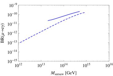
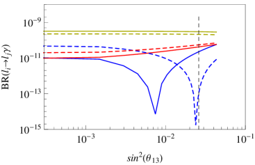
In fig. 1 we recall the generic situation for the type-III seesaw. The dashed and full line correspond to the 2- and 3-generation model, respectively. Only a certain range for $M_{\rm Seesaw}$ is allowed. The lower bounds stem from the fact that the gauge couplings become non-perturbative at the GUT-scale whereas the upper bounds are due to non-perturbative Yukawa couplings at the GUT-scale Esteves:2010ff . Every $\bf 24$-plet contributes with $\Delta b_{i}=5$ to the beta functions of the gauge couplings $g_{i}$ and, thus, obviously the possible range is larger for the 2-generation case compared to the 3-generation case.

Figure 2: BR($\mu\to e\gamma$) (blue), BR($\tau\to e\gamma$) (red) and BR($\tau\to\mu\gamma$) (yellow) over the reactor angle $\theta_{13}$ for real parameters with Dirac phases $\delta=0$ (upper left), $\delta=\pi$ (upper right) and $\delta=3\pi/4$ (lower panel). We set $M_{W}=10^{14}\cdot\hbox{$1\hskip-1.2pt\vrule depth=0.0pt,height=6.88889pt,width=0.7pt\vrule depth=0.0pt,height=0.3pt,width=1.19995pt$}_{3}$ and the SUSY parameters as in eq. (29). The dashed line indicates the current best-fit value for $\theta_{13}$.

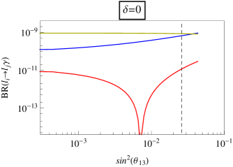
Equations (9) and (17) imply that one can induce special features for the Yukawa couplings when varying $\sin\theta_{13}$, the CP-phases and/or elements of the $R$-matrix as has also been noted in ref. Antusch:2006vw in case of supersymmetric seesaw I models. This has an immediate impact on the flavour mixing entries of the slepton mass parameters as can be seen from eqs. (20) and (21). As an example we show in fig. 2 the dependence on $\theta_{13}$ in the range allowed before the results of DAYA-BAY An:2012eh and RENO Ahn:2012nd assuming three different values for the Dirac-phase $\delta$ and a degenerate mass of $10^{14}$ GeV for the ${\bf 24}$-plets. Note that in this particular case the elements of $R$-matrix do not play any rôle. As can be seen, $\delta$ has to be close to $\pi$ in this case to get BR$(\mu\to e\gamma)$ below the experimental bound. For completeness we note that the small spikes in the plots are numerical artifacts of our iterations procedure.

Figure 3: BR($\mu\to e\gamma$) (blue), BR($\tau\to e\gamma$) (red) and BR($\tau\to\mu\gamma$) (yellow) as function of $\hat{M}_{3}$ with $\theta_{13}$ at the current best-fit value. We have taken $\delta=\pi$, $\hat{M}_{1}=\hat{M}_{2}=10^{14}$ GeV and the other parameters as in eq. (29).

Figure 4: BR($\mu\to e\gamma$) (blue), BR($\tau\to e\gamma$) (red) and BR($\tau\to\mu\gamma$) (yellow) as function of $\sin^{2}\theta_{13}$ in the 2-generation model for $\delta=\pi$, $\hat{M}_{1}=\hat{M}_{2}=10^{14}$ GeV (solid lines) and $\hat{M}_{1}=2\cdot 10^{14}$ GeV, $\hat{M}_{2}=10^{14}$ GeV (dashed lines). The other parameters are as in eq. (29).

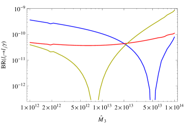
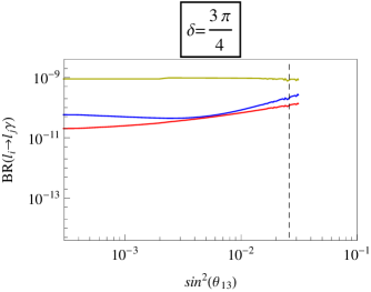
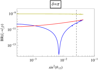
With the recent measurement of $\theta_{13}$ by Daya Bay and RENO one can now relate seesaw parameters from the requirement to respect the bound on $\mu\to e\gamma$. As an example we fix in fig. 3 $\delta=\pi$, $\hat{M}_{1}=\hat{M}_{2}=$ $10^{14}$ GeV and take $R=\hbox{$1\hskip-1.2pt\vrule depth=0.0pt,height=6.88889pt,width=0.7pt\vrule depth=0.0pt,height=0.3pt,width=1.19995pt$}_{3}$. In this case the bound on $\mu\to e\gamma$ is satisfied if $\hat{M}_{3}$ is close to $5\cdot 10^{13}$ GeV. Note however, that the numbers obtained depend on the SUSY point chosen in parameter space. Therefore, one can start to constrain the seesaw parameters only after the discovery and subsequent determination of the SUSY parameters. In fig. 4 we show a similar graph but for the two generation model. The interesting point is that despite the fewer parameters one still has sufficient freedom to suppress the rare lepton decays. One the one hand, this shows the need to determine not only the differences of the neutrino masses squared but also the absolute neutrino mass scale or in other words the mass of the lightest neutrino, as a non-zero value of the latter would rule out the minimal two generation model or requires its extension by non-renormalizable operators. On the other hand it implies that for the exploration of the LHC phenomenology it is sufficient to study the simpler two generation model.

Figure 5: BR($\mu\to e\gamma$) (blue), BR($\tau\to e\gamma$) (red) and BR($\tau\to\mu\gamma$) (yellow) as function of $\sin\phi$ for two 24-plets with masses $\hat{M}_{1}=5\cdot 10^{14}$ GeV and $\hat{M}_{2}=5\cdot 10^{13}$ GeV on the left panel (right panel vice versa $\hat{M}_{1}>\hat{M}_{2}$), $\delta=0$ and the SUSY parameters as in eq. (29).

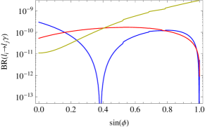
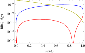
Up to now we have assumed that the $R$-matrix is the unit matrix. In fig. 5 we study the dependence on the $R$-matrix in the two-generation model. We fix the 24-plet masses to $5\cdot 10^{13}$ GeV and $5\cdot 10^{14}$ GeV and vary $\sin(\phi)$. Note that in both cases we have taken $\cos\phi>0$. Instead of taking $\hat{M}_{1}>\hat{M}_{2}$ we could have taken $\cos\phi<0$ in the second plot. As expected, we find that variation of the $R$-matrix provides additional possibilities to suppress BR($\mu\to e\gamma$) below the current experimental bound. Moreover, our results show that one never can exclude this class of models by these measurements as with a sufficient tuning of parameters one can always avoid the bounds.

Figure 6: Comparison of the two-body decays $l_{i}\to l_{j}\gamma$ (left panel) and the-three body decays $l_{i}\to 3l_{j}$ (right panel) for variation of $\sin(\phi_{1})$ at normal neutrino mass hierarchy, Dirac phase $\delta=0$ and a 24-plet hierarchy: $\hat{M}_{1}=10^{15}$ GeV, $\hat{M}_{2}=10^{14}$ GeV and $\hat{M}_{3}=10^{13}$ GeV; $l_{i}$, $l_{j}$ = $\mu$, $e$ (blue); $\tau$, $e$ (red); $\tau$, $\mu$ (yellow).

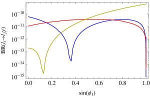
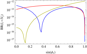
For completeness we compare in fig. 6 the branching ratios of the two body decays $l_{i}\to l_{j}\gamma$ to the ones for the three body decays $l_{i}\to 3l_{j}$ in the three-generation model. Similar to the seesaw type I case Arganda:2005ji we see that both decay classes show the same dependence on the underlying parameters, since in case of the three body decays the photon contribution dominates. We have checked that this also holds for the two-generation model.

III.2 Testing flavour structures at the LHC

We have seen in the previous section that one can choose the seesaw parameters such that the experimental constraints on the rare leptons decays are fulfilled. In this section we address the question if there are any possibilities to test these models for such parameter choices at the LHC. As we will demonstrate there are indeed favorable SUSY parameter regions where one can observe the corresponding flavour violating decays of supersymmetric particles.

The branching ratios of the lepton flavour violating decays of sleptons and neutralinos are governed by the same entries in the slepton mass matrix as the rare lepton decays, i.e. the ones given in eqs. (20) and (21). Therefore both classes of decays show the same dependence on the seesaw parameters.

At the LHC one has to study cascade decays containing sequences of the form $\tilde{\chi}^{0}_{2}\to\tilde{l}_{k}^{\pm}l^{\mp}_{j}\to l_{i}^{\pm}l^{\mp}_{j}\tilde{\chi}^{0}_{1}$ with $i\neq j$ Hinchliffe:2000np ; Deppisch:2004pc ; Bartl:2005yy ; Andreev:2006sd ; delAguila:2008iz ; Hirsch:2008dy ; Carquin:2008gv ; Esteves:2009vg . Moreover, the nature of the neutralinos should be dominantly gaugino like and the mass difference should be small enough to suppress the decay into $h^{0}$. This requires a certain hierarchy between the neutralino mass parameters and the slepton mass parameters which is roughly given by $|\mu|\gg M_{2}\raise 1.29167pt\hbox{$\;>$\kern-7.5pt\raise-4.73611pt\hbox{$\sim\;$}}m_{\tilde{l}}\raise 1.29167pt\hbox{$\;>$\kern-7.5pt\raise-4.73611pt\hbox{$\sim\;$}}M_{1}$ where the ordering of $M_{1}$ and $M_{2}$ can be interchanged.

As the scaling of the lepton flavour violating decays of SUSY particles is similar to the one of the rare lepton decays in this class of models we use the following strategy to enhance the rates for $\tilde{\chi}^{0}_{2}\to\tilde{e}^{\pm}\mu^{\mp}\chi^{0}_{1}$, $\tilde{\chi}^{0}_{2}\to\tilde{e}^{\pm}\tau^{\mp}\chi^{0}_{1}$ and $\tilde{\chi}^{0}_{2}\to\tilde{\mu}^{\pm}\tau^{\mp}\chi^{0}_{1}$: for a given point in the SUSY parameter space we choose the seesaw parameters in the following way: we fix the $R$-matrix to be either $1\hskip-1.2pt\vrule depth=0.0pt,height=6.88889pt,width=0.7pt\vrule depth=0.0pt,height=0.3pt,width=1.19995pt$ or as in eq. (18), depending whether we work in the two- or three-generation seesaw model. Next we fix the relative size of various entries of $Y_{W}$ such that the neutrino mixing matrix is tribimaximal. Note, that a non-zero $\theta_{13}$ changes the neutralino branching ratios only slightly and, thus, its effect can be neglected her. In the third step both $Y_{W}$ and $M_{W}$ are rescaled until the correct neutrino masses are obtained and $10^{12}\cdot\text{BR}(\mu\to e\gamma)$ is in the interval $[2.2,2.4]$. In this way one obtains the maximum rate for the decay $\tilde{\chi}^{0}_{2}\to\tilde{e}^{\pm}\mu^{\mp}\chi^{0}_{1}$ which is the cleanest at the LHC Andreev:2006sd ; delAguila:2008iz . With a further variation of the entries in $Y_{W}$ one could increase the final states containing a $\tau$ lepton. However, we have checked for couple of points in the SUSY parameter space that this would only lead to an relative increase of about ten per-cent for the corresponding rates. We have not pursued this further as this is at most of the order of the expected theoretical uncertainty on the SUSY cross section, which is about 10-20 per-cent, see e.g. Beenakker:2011sf ; Kramer:2012bx ; Hollik:2012rc ; Langenfeld:2012ti and refs. therein. In the following examples we have checked that the bounds on SUSY particles are fulfilled Chatrchyan:2012jx ; CMS:2012mfa ; ATLAS:2012rz ; ATLAS:2012ms .

Figure 7: BR($\widetilde{\chi}^{0}_{2}\to\widetilde{\chi}^{0}_{1}l_{i}l_{j}$) and selected masses as function of $M_{1/2}$ for $m_{0}=250$ GeV, $A_{0}=0$, $\tan\beta=10$ and $\mu>0$. Left plot: BR($\widetilde{\chi}^{0}_{2}\to\widetilde{\chi}^{0}_{1}\mu e$) (blue), BR($\widetilde{\chi}^{0}_{2}\to\widetilde{\chi}^{0}_{1}\tau e$) (red) and BR($\widetilde{\chi}^{0}_{2}\to\widetilde{\chi}^{0}_{1}\tau\mu$) (yellow); right plot: $\widetilde{\chi}^{0}_{2}$ (orange), $\widetilde{\chi}^{0}_{1}$ (red), $\widetilde{l}_{1,2,3}$ (blue dotted) and $\widetilde{l}_{4,5,6}$ (green dotted). The neutrino parameters are at tri-bi-maximal values, normal neutrino mass hierarchy and $R=\mathds{1}$; $M_{W}$ is varied to fit BR($\mu\to e\gamma$) close to the experimental bound.

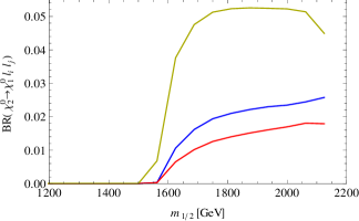
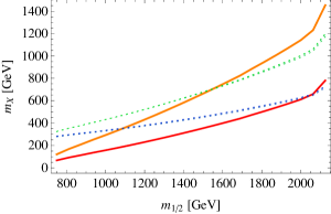
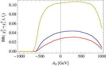
The branching ratios of the lepton flavour violating decays can reach up to a few per-cent as shown in fig. 7. The structure of the RGEs implies that the three heaviest sleptons are essentially $\tilde{l}_{L}$ even though there can be sizeable mixing between the stau states. The latter mixing is the main source of the LFV decays for $M_{1/2}\raise 1.29167pt\hbox{$\;<$\kern-7.5pt\raise-4.73611pt\hbox{$\sim\;$}}1550$ GeV where only the three lightest sleptons appear in the $\tilde{\chi}^{0}_{2}$ decays. The hierarchy BR($\widetilde{\chi}^{0}_{2}\to\widetilde{\chi}^{0}_{1}\tau\mu)>$ BR($\widetilde{\chi}^{0}_{2}\to\widetilde{\chi}^{0}_{1}\mu e)>$ BR($\widetilde{\chi}^{0}_{2}\to\widetilde{\chi}^{0}_{1}\tau e$) is a consequence of the structure of $Y_{W}$ needed to explain the neutrino data. The change of the spectrum has two main sources: (i) $M_{1/2}$ enters the RGEs for the slepton mass parameters. (ii) The requirement that BR$(\mu\to e\gamma)$ to be in above interval implies that the seesaw scale becomes a function of $M_{1/2}$. Changing the seesaw scale has a major impact on spectrum as discussed in detail in ref. Esteves:2010ff . Similar features show up in the 2-generation model as exemplified in fig. 8 where we show the LFV $\widetilde{\chi}^{0}_{2}$ decay branching ratios as a function of $A_{0}$. In this model one can find LFV branching ratios of up to 10 per-cent. The main reason for this are the different kinematics for the same mSUGRA input because changing the number of seesaw particles implies changes in the RGEs of the slepton and gaugino mass parameters as discussed above.

Figure 8: BR($\widetilde{\chi}^{0}_{2}\to\widetilde{\chi}^{0}_{1}\mu e$) (blue), BR($\widetilde{\chi}^{0}_{2}\to\widetilde{\chi}^{0}_{1}\tau e$) (red) and BR($\widetilde{\chi}^{0}_{2}\to\widetilde{\chi}^{0}_{1}\tau\mu$) (yellow) in the 2-generation model as function of $A_{0}$ for $m_{0}=250$ GeV, $M_{1/2}=1800$ GeV, $\tan\beta=10$ and $\mu>0$. The seesaw parameters are fixed as explained in the text.

Figure 9: Grid calculation of $\sigma(\widetilde{\chi}^{0}_{2})\times\text{BR}(\widetilde{\chi}^{0}_{2}\to\widetilde{\chi}^{0}_{1}\mu e$) (blue), $\sigma(\widetilde{\chi}^{0}_{2})\times\text{BR}(\widetilde{\chi}^{0}_{2}\to\widetilde{\chi}^{0}_{1}\tau e$) (red) and $\sigma(\widetilde{\chi}^{0}_{2})\times\text{BR}(\widetilde{\chi}^{0}_{2}\to\widetilde{\chi}^{0}_{1}\tau\mu$) (yellow) in femtobarn over $M_{1/2}$ for different values of $m_{0}$; $A_{0}=0$, $\tan\beta=10$ and $\mu>0$. The seesaw parameters are fixed as explained in the text.

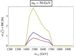
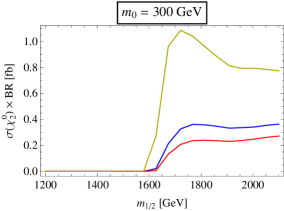
We concentrate in the following on the two generation model as here the signal is somewhat larger than in the three generation model. At the LHC $\widetilde{\chi}^{0}_{2}$ is mainly produced in the cascade decays of squarks and gluinos. In fig. 9 we show $\sigma\times$BR as a function of $M_{1/2}$ fixing the other parameters for two values of $m_{0}$, $A_{0}=0$, $\tan\beta=10$, $\mu>0$ and $\sqrt{s}=14$ TeV. In addition, we used $\hat{M}_{1}=\hat{M}_{2}=2.5\cdot 10^{13}$ GeV as well as $Y_{W,11}=Y_{W,12}=-Y_{W,13}=-5.252\cdot 10^{-2}$, $Y_{W,21}=0$ and $Y_{W,22}=Y_{W,23}=-1.547\cdot 10^{-1}$. Here we have summed over all possibilities to produce squarks and gluinos and we require that the two leptons from $\widetilde{\chi}^{0}_{2}$ are the only ones in the event. For the calculation of the cross section we have used the LHC-FASER package Dreiner:2010gv ; benfaser . One sees that the signal cross section before putting any cuts can be at most a few fb which gives at most a few hundred events even for an integrated luminosity of 300 fb^-1.

Figure 10: Invariant mass distributions for the signal and SUSY background for final states containing $\mu$, $e$ (left plot) or $\tau$, $\mu$ (right plot), missing transverse energy and at least two jets in the final state for a luminosity of $300\text{ fb}^{-1}$, $m_{0}=50$ GeV, $M_{1/2}=1484$ GeV, $A_{0}=0$, $\tan\beta=10$ and $\mu>0$.

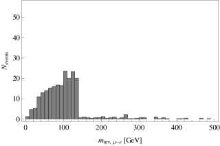
This naturally leads to the question if such a signal can be observed at all. For this reason we have performed a Monte Carlo study at the parton level taking $m_{0}=50$ GeV, $M_{1/2}=1484$ GeV, $A_{0}=0$, $\tan\beta=10$ and $\mu>0$ corresponding to maximum of the signal in fig. 9. For the generation of the events we use WHIZARD Kilian:2007gr . The corresponding signal cross sections are 1.4, 0.8 and 3.8 fb for the final states containing $e\mu$, $e\tau$ and $\mu\tau$, respectively. Related studies have been performed in refs. Hinchliffe:2000np ; Hisano:2002iy ; Andreev:2006sd where it has been shown that one can reduce the SM background sufficiently. However, to our knowledge the SUSY background has not yet been taken into account. This will be also considered here. The main SM background are due $t\bar{t}$, $VV$ and $Vjj$ ($V=W,Z$) production. In ref. juliaharz , where a detector study for the $\mu\tau$ channel has been performed for $\sqrt{s}=10$ TeV, it has been shown that the SM background can reduced significantly by requiring a cut on the missing transverse energy ${E_{T}/}\hskip 7.11317pt>140$ GeV and a cut on the effective mass $M_{eff}>400$ GeV where

$$M_{eff}\equiv{E_{T}/}\hskip 7.11317pt+\sum_{i=1}^{4}p^{jet}_{T}\,.+\sum_{j}p^{l}_{T}$$

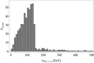
The first sum is over the transverse momentum of the four hardest jets and the second one over the transverse momentum of all leptons. We have adjusted these cuts for the case $\sqrt{s}=14$ TeV and use ${E_{T}/}\hskip 7.11317pt>150$ $M_{eff}>1200$ GeV. Moreover we require that the event contains exactly two leptons and no $b$-jets. This reduces the SM-background to a negligible level. The main SUSY background is due to charginos and $W$-bosons produced in the SUSY cascade decays. In contrast to the signal these events stem in general from cascade decays of different squarks and/or gluinos. Therefore, if one plots the differential cross section as a function of the invariant lepton mass $m_{ll^{\prime}}=\sqrt{(p_{l}+p_{l^{\prime}})^{2}}$ one gets a triangle for the peak and a flat distribution from the background. We have simulated the combination of signal with SUSY background using the dominant production mechanism which is in this case squark-squark production as the squarks are much lighter than the gluino yielding about 80 per-cent of the total cross section. The results for an integrated luminosity of 300 fb^-1 are shown in fig. 10 where we have cut the range of $m_{ll^{\prime}}$ at 500 GeV even though the SUSY background continues flat until about 1 TeV. As can be seen, one gets approximately the triangular shape of the signal with the edge at

$$m^{2}_{ll^{\prime}}=\frac{(m^{2}_{\tilde{\chi}^{0}_{2}}-m^{2}_{\tilde{l}})(m^{2}_{\tilde{l}}-m^{2}_{\tilde{\chi}^{0}_{2}})}{m^{2}_{\tilde{l}}}$$ (30)

where the lepton masses have been neglected. The edge clearly indicates the consecutive two body decays giving a first hint on the mass ordering. As the sleptons have different masses, they give somewhat different values for the edges which are collected in Tab. 1.

Table 1: Edges, as given in eq. (30), of the invariant lepton masses due to the individual sleptons. The two neutralino masses are 344.6 GeV and 647.0 GeV

slepton	mass [GeV]	$m_{ll^{\prime}}$ [GeV]
$\tilde{l}_{1}$	377.9	213.0
$\tilde{l}_{2,3}$	386.0	233.9
$\tilde{l}_{4}$	621.9	148.3
$\tilde{l}_{5}$	625.1	139.3
$\tilde{l}_{6}$	625.9	136.7

Figure 10 clearly shows that in this case the SUSY background is negligible compared to the signal. Note that the light sleptons hardly contribute to the signal as argued above and, thus, the edges are essentially due to the heavier sleptons. In case of the $\tau\mu$ final state the two edges could be guessed but it will require high luminosity and a finer binning to disentangle the resulting double edge structure due to the contributions of the different sleptons Bartl:2005yy .

IV Conclusions

We have studied supersymmetric variants of the seesaw type III model. At the electroweak scale the particle content is the same as in the MSSM. At the seesaw scale(s) the particles have been included in a 24-plet to ensure unification of the gauge couplings. In this way one ends up with a combination of seesaw type III combined with type I where the latter gives sub-dominant contribution if $SU(5)$-GUT conditions for the corresponding Yukawa couplings are assumed. We have considered two variants of this model using either two or three generation of 24-plets. The latter case is heavily constrained by the experimental bound on $\mu\to e\gamma$. However, as we have shown there are various ways to obtain cancellations between different contributions so the bound can be respected: here the Dirac phase of the neutrino sector enters as well as the mass hierarchy of the seesaw particles and their mixing properties. Even though the measurement of the reactor angle $\theta_{13}$ gives an additional constraint, the model still has sufficient many parameters to be consistent with all experimental data. In the two generation model the constraints due to the rare lepton decays are less severe and can be more easily accommodated.

We have also investigated the question to which extent lepton flavour violating signals can be seen at the LHC. The current experimental bounds on SUSY particles imply that within a unified model such as the mSugra squarks and gluinos must be in the TeV range. As the main signal is in the cascade decays of these particles one gets at most a few fb for the signal. The corresponding part of the parameter space is for small $m_{0}$ and large $m_{1/2}$ if the seesaw parameters are chosen such that BR$(\mu\to e\gamma)$ is close to its experimental bound. One can turn this around: if the bound BR$(\mu\to e\gamma)$ is increased by an order of magnitude than it is rather unlikely that LHC finds LFV in SUSY decays in this class of models.

References

- (1) E. Ma, Phys.Rev.Lett. 81, 1171 (1998), arXiv:hep-ph/9805219.
- (2) P. Minkowski, Phys.Lett. B67, 421 (1977).
- (3) T. Yanagida, Horizontal symmetry and masses of neutrinos, in KEK lectures, ed. O. Sawada and A. Sugamoto, 1979.
- (4) M. Gell-Mann, P. Ramond, and R. Slansky, Complex spinors and unified theories, in Supergravity, ed. P. van Niewenhuizen and D. Freedman (North Holland), 1979.
- (5) R. N. Mohapatra and G. Senjanovic, Phys.Rev.Lett. 44, 912 (1980).
- (6) J. Schechter and J. Valle, Phys.Rev. D22, 2227 (1980).
- (7) T. Cheng and L.-F. Li, Phys.Rev. D22, 2860 (1980).
- (8) R. Foot, H. Lew, X. He, and G. C. Joshi, Z.Phys. C44, 441 (1989).
- (9) S. Weinberg, Phys.Rev.Lett. 43, 1566 (1979).
- (10) S. Weinberg, Phys.Rev. D22, 1694 (1980).
- (11) E. Witten, Nucl.Phys. B188, 513 (1981).
- (12) S. Dimopoulos, S. Raby, and F. Wilczek, Phys.Rev. D24, 1681 (1981).
- (13) L. E. Ibanez and G. G. Ross, Phys.Lett. B105, 439 (1981).
- (14) W. J. Marciano and G. Senjanovic, Phys.Rev. D25, 3092 (1982).
- (15) M. Einhorn and D. Jones, Nucl.Phys. B196, 475 (1982).
- (16) U. Amaldi, W. de Boer, and H. Furstenau, Phys.Lett. B260, 447 (1991).
- (17) P. Langacker and M.-x. Luo, Phys.Rev. D44, 817 (1991).
- (18) J. R. Ellis, S. Kelley, and D. V. Nanopoulos, Phys.Lett. B260, 131 (1991).
- (19) L. E. Ibanez and G. G. Ross, Phys.Lett. B110, 215 (1982).
- (20) J. Hisano, M. M. Nojiri, Y. Shimizu, and M. Tanaka, Phys.Rev. D60, 055008 (1999), arXiv:hep-ph/9808410.
- (21) A. Rossi, Phys.Rev. D66, 075003 (2002), arXiv:hep-ph/0207006.
- (22) M. R. Buckley and H. Murayama, Phys.Rev.Lett. 97, 231801 (2006), arXiv:hep-ph/0606088.
- (23) M. Hirsch, S. Kaneko, and W. Porod, Phys.Rev. D78, 093004 (2008), arXiv:0806.3361.
- (24) F. Borzumati and T. Yamashita, Prog.Theor.Phys. 124, 761 (2010), arXiv:0903.2793.
- (25) J. Esteves, J. Romão, M. Hirsch, F. Staub, and W. Porod, Phys.Rev. D83, 013003 (2011), arXiv:1010.6000.
- (26) F. Borzumati and A. Masiero, Phys.Rev.Lett. 57, 961 (1986).
- (27) J. Hisano, T. Moroi, K. Tobe, M. Yamaguchi, and T. Yanagida, Phys.Lett. B357, 579 (1995), arXiv:hep-ph/9501407.
- (28) J. Hisano, T. Moroi, K. Tobe, and M. Yamaguchi, Phys.Rev. D53, 2442 (1996), arXiv:hep-ph/9510309.
- (29) J. R. Ellis, J. Hisano, M. Raidal, and Y. Shimizu, Phys.Rev. D66, 115013 (2002), arXiv:hep-ph/0206110.
- (30) F. Deppisch, H. Pas, A. Redelbach, R. Rückl, and Y. Shimizu, Eur.Phys.J. C28, 365 (2003), arXiv:hep-ph/0206122.
- (31) S. Petcov, S. Profumo, Y. Takanishi, and C. Yaguna, Nucl.Phys. B676, 453 (2004), arXiv:hep-ph/0306195.
- (32) E. Arganda and M. J. Herrero, Phys.Rev. D73, 055003 (2006), arXiv:hep-ph/0510405.
- (33) S. Petcov, T. Shindou, and Y. Takanishi, Nucl.Phys. B738, 219 (2006), arXiv:hep-ph/0508243.
- (34) S. Antusch, E. Arganda, M. Herrero, and A. Teixeira, JHEP 0611, 090 (2006), arXiv:hep-ph/0607263.
- (35) F. Deppisch and J. Valle, Phys.Rev. D72, 036001 (2005), arXiv:hep-ph/0406040.
- (36) M. Hirsch, J. Valle, W. Porod, J. Romão, and A. Villanova del Moral, Phys.Rev. D78, 013006 (2008), arXiv:0804.4072.
- (37) E. Arganda, M. Herrero, and A. Teixeira, JHEP 0710, 104 (2007), arXiv:0707.2955.
- (38) F. Deppisch, T. Kosmas, and J. Valle, Nucl.Phys. B752, 80 (2006), arXiv:hep-ph/0512360.
- (39) C. Biggio and L. Calibbi, JHEP 1010, 037 (2010), arXiv:1007.3750.
- (40) P. Fileviez Perez, Phys.Rev. D76, 071701 (2007), arXiv:0705.3589.
- (41) R. Mohapatra, N. Okada, and H.-B. Yu, Phys.Rev. D78, 075011 (2008), arXiv:0807.4524.
- (42) A. Abada, A. Figueiredo, J. Romao, and A. Teixeira, JHEP 1108, 099 (2011), arXiv:1104.3962.
- (43) ATLAS Collaboration, G. Aad et al., Phys.Lett. B710, 49 (2012), arXiv:1202.1408.
- (44) CMS Collaboration, S. Chatrchyan et al., Phys.Lett. B710, 26 (2012), arXiv:1202.1488.
- (45) P. Bechtle et al., JHEP 1206, 098 (2012), arXiv:1204.4199.
- (46) O. Buchmueller et al., (2012), arXiv:1207.7315.
- (47) M. Hirsch, F. Joaquim, and A. Vicente, (2012), arXiv:1207.6635.
- (48) U. Ellwanger and C. Hugonie, Adv.High Energy Phys. 2012, 625389 (2012), arXiv:1203.5048.
- (49) J. F. Gunion, Y. Jiang, and S. Kraml, Phys.Lett. B710, 454 (2012), arXiv:1201.0982.
- (50) G. G. Ross and K. Schmidt-Hoberg, Nucl.Phys. B862, 710 (2012), arXiv:1108.1284.
- (51) U. Ellwanger, C. Hugonie, and A. M. Teixeira, Phys.Rept. 496, 1 (2010), arXiv:0910.1785.
- (52) S. Choi, . Miller, D.J., and P. Zerwas, Nucl.Phys. B711, 83 (2005), arXiv:hep-ph/0407209.
- (53) C. Cheung, L. J. Hall, D. Pinner, and J. T. Ruderman, (2012), arXiv:1211.4873.
- (54) A. Delgado, C. Kolda, and A. de la Puente, Phys.Lett. B710, 460 (2012), arXiv:1111.4008.
- (55) G. G. Ross, K. Schmidt-Hoberg, and F. Staub, JHEP 1208, 074 (2012), arXiv:1205.1509.
- (56) S. K. Kang, T. Morozumi, and N. Yokozaki, JHEP 1011, 061 (2010), arXiv:1005.1354.
- (57) J. Casas and A. Ibarra, Nucl.Phys. B618, 171 (2001), arXiv:hep-ph/0103065.
- (58) A. Ibarra and G. G. Ross, Phys. Lett. B591, 285 (2004), arXiv:hep-ph/0312138.
- (59) P. H. Chankowski, J. R. Ellis, S. Pokorski, M. Raidal, and K. Turzynski, Nucl. Phys. B690, 279 (2004), arXiv:hep-ph/0403180.
- (60) B. Dutta and R. N. Mohapatra, Phys. Rev. D68, 056006 (2003), arXiv:hep-ph/0305059.
- (61) A. Masiero, S. Vempati, and O. Vives, New J. Phys. 6, 202 (2004), arXiv:hep-ph/0407325, Focus Issue on ’Neutrino Physics’ edited by F. Halzen, M. Lindner and A. Suzuki.
- (62) A. Ibarra, JHEP 0601, 064 (2006), arXiv:hep-ph/0511136.
- (63) A. Bartl, W. Majerotto, W. Porod, and D. Wyler, Phys.Rev. D68, 053005 (2003), arXiv:hep-ph/0306050.
- (64) W. Porod, Comput. Phys. Commun. 153, 275 (2003), arXiv:hep-ph/0301101.
- (65) W. Porod and F. Staub, Comput.Phys.Commun. 183, 2458 (2012), arXiv:1104.1573.
- (66) F. Staub, (2008), arXiv:0806.0538.
- (67) F. Staub, Comput. Phys. Commun. 181, 1077 (2010), arXiv:0909.2863.
- (68) F. Staub, Comput. Phys. Commun. 182, 808 (2011), arXiv:1002.0840.
- (69) F. Staub, (2012), arXiv:1207.0906.
- (70) F. Staub, T. Ohl, W. Porod, and C. Speckner, Comput.Phys.Commun. 183, 2165 (2012), arXiv:1109.5147.
- (71) W. Kilian, T. Ohl, and J. Reuter, Eur.Phys.J. C71, 1742 (2011), arXiv:0708.4233.
- (72) D. Forero, M. Tortola, and J. Valle, (2012), arXiv:1205.4018.
- (73) MEG collaboration, J. Adam et al., Phys.Rev.Lett. 107, 171801 (2011), arXiv:1107.5547.
- (74) DAYA-BAY Collaboration, F. An et al., Phys.Rev.Lett. 108, 171803 (2012), arXiv:1203.1669.
- (75) RENO collaboration, J. Ahn et al., Phys.Rev.Lett. 108, 191802 (2012), arXiv:1204.0626.
- (76) L. Calibbi, D. Chowdhury, A. Masiero, K. Patel, and S. Vempati, (2012), arXiv:1207.7227.
- (77) I. Hinchliffe and F. Paige, Phys.Rev. D63, 115006 (2001), arXiv:hep-ph/0010086.
- (78) F. Deppisch, J. Kalinowski, H. Pas, A. Redelbach, and R. Rückl, (2004), arXiv:hep-ph/0401243.
- (79) A. Bartl et al., Eur.Phys.J. C46, 783 (2006), arXiv:hep-ph/0510074.
- (80) Y. Andreev, S. Bityukov, N. Krasnikov, and A. Toropin, Phys.Atom.Nucl. 70, 1717 (2007), arXiv:hep-ph/0608176.
- (81) F. del Aguila et al., Eur.Phys.J. C57, 183 (2008), arXiv:0801.1800.
- (82) E. Carquin, J. Ellis, M. Gomez, S. Lola, and J. Rodriguez-Quintero, JHEP 0905, 026 (2009), arXiv:0812.4243.
- (83) J. Esteves et al., JHEP 0905, 003 (2009), arXiv:0903.1408.
- (84) W. Beenakker et al., JHEP 1201, 076 (2012), arXiv:1110.2446.
- (85) M. Kramer et al., (2012), arXiv:1206.2892.
- (86) W. Hollik, J. M. Lindert, and D. Pagani, (2012), arXiv:1207.1071.
- (87) U. Langenfeld, S.-O. Moch, and T. Pfoh, (2012), arXiv:1208.4281.
- (88) CMS Collaboration, S. Chatrchyan et al., JHEP 1210, 018 (2012), arXiv:1207.1798.
- (89) CMS Collaboration, S. Chatrchyan et al., (2012), arXiv:1207.1898.
- (90) ATLAS Collaboration, G. Aad et al., (2012), arXiv:1208.0949.
- (91) ATLAS Collaboration, G. Aad et al., (2012), arXiv:1208.4688.
- (92) H. K. Dreiner, M. Kramer, J. M. Lindert, and B. O’Leary, JHEP 1004, 109 (2010), arXiv:1003.2648.
- (93) B. O’Leary, LHC-FASER, https://github.com/benoleary/LHC-FASER, 2012.
- (94) J. Hisano, R. Kitano, and M. M. Nojiri, Phys.Rev. D65, 116002 (2002), arXiv:hep-ph/0202129.
- (95) J. Harz, Lepton-Flavor-Verletzung am ATLAS-Experiment am Beispiel des Zerfalls , diploma thesis, University of Würzburg, 2010.