What is PINGSoft?

The PINGS software, or PINGSoft, is a set of IDL routines designed to visualise, manipulate and analyse in a simply way Integral Field Spectroscopic (IFS) data regardless of the original instrument and spaxel size/shape, it is able to run on practically any computer platform with minimal library requirements (Rosales-Ortega, 2011).

PINGSoft 2 is a relatively major upgrade with respect to the first version. The overall functionality and layout have been improved, while the command syntax has been simplified. This version includes new routines that offer additional extraction options and some level of analysis. PINGSoft includes basic tools to visualise spatially and spectrally IFS data, to extract regions of interest by hand or within a given geometric aperture, to integrate the spectra within a given region, and to perform simple analysis to the IFS data. Additionally, some miscellaneous codes useful for generic tasks performed in astronomy and spectroscopy are also included. PINGSoft is optimised for a fast visualisation rendering, it can be adapted to work with practically any IFS data/instrument, and is adapted to work natively with the CALIFA survey data.

New features

• A new Graphical User Interface (widget) for interactive visualisation of the spaxels and spectra of a 3D cube or RSS file.

• The data can be convolved with a full set of narrow and broad-band filters for visualization and/or analysis purposes. The filter used to visualize the data is shown on the spectral window.

• Elliptical apertures for spectra extraction are now supported (for any ellipticity, size and PA).

• Radial binning extraction with either fixed bins or based on a S/N floor.

• Spectra extraction and integration based on a user-given mask.

• Conic or hyperbolic aperture extractions for any PA, size and angle.

• Spectra integration based on S/N on continuum and/or emission line features.

• Voronoi binning based on the method developed by Cappellari & Copin (2003).

• Intrinsic velocity field correction using a wavelength cross-correlation.

• Furthermore, the PINGSoft routines can now read 3D cubes or RSS files indistinctively. The syntax is much simpler, e.g. to load a RSS file the user only needs to include the name of the FITS file (and omit the position table) if the format is the following: OBJECT.fits, OBJECT.pt.txt, and both files reside on the same directory.

In this document, we introduce the new visualisation tools of PINGSoft. We also list all the available routines for spectra extraction, analysis and manipulation of IFS data. A detailed description of the remaining routines can be found in the PINGSoft 2 User’s Guide, together with detailed installation instructions, all available at the project webpage:

http://califa.caha.es/pingsoft

The PINGSoft integral field spectroscopy software

All PINGSoft routines are called via command lines in a terminal running IDL. The syntax and online help for any program can be obtained by entering the name of the procedure without any parameter or keyword, With the exception of the visualisation widget: view_ifs, /help.

Additionally, in the PINGSoft webpage you can download the pingsoft_examples/ directory which includes some 3D cubes and RSS example files. I recommend the user to download this example data and follow the instructions in the README.pro file in order to get a first insight of the main PINGSoft routines. All the example commands used in this document can be found in the README.pro file of the pingsoft_examples/ directory.

IFS visualisation

view_ifs

This routine provides a spatial and spectral interactive visualisation widget for 3D cubes and RSS IFS files. If the command is simply entered in the IDL terminal:

IDL> view_ifs

it prompts for an input FITS file using a dialog window. Otherwise, the input file can be passed directly to the command as the first parameter:

IDL> view_ifs, ’OBJECT.fits’

The widget will be displayed automatically if the input file is a 3D FITS cube. If the input FITS is a RSS file, the program will look in the same directory for a position table named OBJECT.pt.txt and will launch the widget if the file exists. If this is not the case, the program will exit with an error. The user can define the name of the corresponding position table using the PT parameter:

IDL> view_ifs, ’OBJECT.fits’, PT=’PosTable.txt’

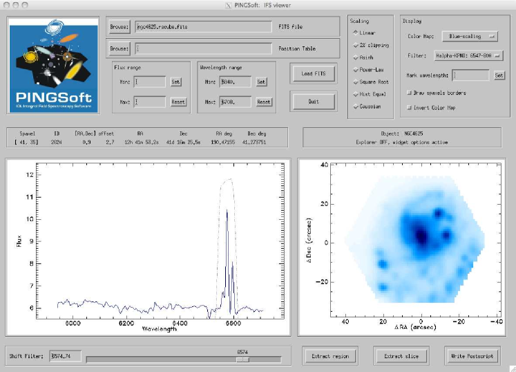
Figure 1: Screen shot of the visualisation widget launched by the view_ifs command, displaying the 3D cube of the galaxy NGC 4625 included in the pingsoft_examples/ directory.

The view_ifs widget is shown in Figure 1, displaying the 3D cube file ngc4625.rscube.fits included in the pingsoft_examples/ directory. The widget displays two main panels, on the right a visualisation of the spatial distribution of spaxels (or field-of-view, FoV). The color-scaling corresponds to a narrow/broad-band image of a transmission filter convolved with the data at a given wavelength (shown as a dotted-curve in the spectral window). The spatial units are assumed to be arcseconds in a standard North (up) East (left) configuration. The left panel shows the spectrum of the spaxel corresponding to the position of the mouse, the wavelength range is extracted from the information on the FITS header. The corresponding spaxel position, ID and offsets are shown on the top of the spectral window. Optionally, if the WCS is included in the FITS header, the RA and Dec are also shown in sexagesimal and degree units, a mouse LEFT-click prints the same spaxel information on the IDL terminal where the program was called.

USAGE: At first glance, the usage of the view_ifs widget may seem ‘‘tricky’’, but it is easy to get used to: when the widget is launched, the user can explore spatially and spectrally the IFS data but the widget options will be inactive. To have access to the widget options, the user needs to RIGHT-click with the mouse over the FoV panel. When the widget options are changed the spectral explorer will become active again and the widget options will be unavailable. To active/deactivate the widget options the user only needs to RIGHT-click over the FoV to switch between the explorer ON/OFF options. The status bar above the FoV panel (below the object name) will indicate whether the explorer is active or not.

Several options are available to visualise the data, including different intensity scalings, color maps, a set of different narrow and broad-band filters in the optical to generate the visualisation in the FoV panel, the choice to define the flux intensity and spectral ranges, to drawing the contour of the spaxels, to invert the color-map, etc. Note that the central wavelength of the filter used to display the data can be shifted to any position along the spectral range, either by using the slider or by setting the wavelength in the corresponding field. New FITS (position tables) files can be loaded using the corresponding fields at the top-center of the widget, and by pressing the ‘‘Load FITS’’ button.

Extract region: By pressing this button, all the subsequent LEFT-clicks over the FoV panel will mark and select the spaxels to be extracted. When the program is terminated (by RIGHT-click) the following files are created:

      Extracted RSS:   OBJECT_rss.fits    (Extracted RSS of the selected spaxels)
     Position table:   OBJECT_rss.pt.txt  (Position table of the new RSS file)
   Integrated ASCII:   OBJECT_integ.txt   (Integrated spectrum in ASCII format)
               FITS:   OBJECT_integ.fits  (Integrated spectrum in FITS format)
         Postscript:   OBJECT_integ.eps   (Postscript image of the integrated spectrum)
        IDL indices:   OBJECT_index.txt   (IDL indices of the selected spaxels)

shown in the IDL terminal window, while the spectral panel will show the integrated spectrum of the selected spaxels.

Extract slice: Pressing this button will invoke the extract_filter command with the filter and central wavelength parameters as the current values displayed in the widget. This will create a FITS image file called OBJECT_slice.fits as reported in the status bar, additional information will be shown in the IDL terminal window. WARNING: This option is only available for 3D cubes and RSS with a rectangular-contiguous grid.

Write Postscript: Pressing this button will create an encapsulated Postscript image (OBJECT_FoV.eps) of the FoV panel with the current display options of the widget. The name of the file will be reported in the status bar and terminal window.

Mark wavelength: Use this field to enter one or several wavelengths at which a vertical line will be drawn in the spectral panel. This option is useful when trying to identify features at known wavelengths. The input formats can be of the form:

Mark wavelength: 6563
                 5007, 6563
                 5895*1.002          (e.g. known redshifts)
                 [4310,5876]*1.0015

Figure 2: Screen shot of the visualisation widget for a CALIFA datacube, the bad-pixels are displayed in a light-blue color in the spectral panel.

CALIFA data: When a CALIFA data file is loaded with view_ifs, the display color is changed to the CALIFA-special color map, the routine identifies automatically the different FITS extensions (HDUs) of the CALIFA format (for both RSS and 3D cube versions). The BADPIX extension is shown in the spectral panel simultaneously with the flux data, the bad-pixels are displayed in a light-blue color as shown in Figure 2.

Size and resolution: The view_ifs widget may not display properly for screens with resolutions lower than 1400$\times$800. In this case, the user can modify by hand the size of the widget to fit their own screen resolution by editing the first entries in the widget_param.pro routine.

view_3D

This routine is the command-line version of view_ifs, it provides a 2D interactive visualisation of the spaxels and spectra of a 3D cube or a RSS file and its corresponding position table. However, the visualisation is performed in two standard IDL windows (i.e. a lighter visualisation option). All display and interactive options are similar to view_ifs (with the exception of the ‘‘Extract slice’’ option), the command is terminated by RIGHT-click on the FoV window.

A mouse MIDDLE-button click is equivalent to the ‘‘Extract region’’ button in the widget, it prompts in the IDL terminal for a PREFIX used to generate the new series of files, all the subsequent LEFT-clicks over the FoV window will mark and select the spaxels to be extracted. The extraction is performed by RIGHT-click on the FoV window, the extracted files are displayed in the terminal window, while the spectral window shows the integrated spectrum of the selected spaxels.

Additional features:

1. The view_3D routine accepts the /LARGE keyword, which displays a much larger FoV window.

2. The user can specifying the FITS extension to read using the EXTENSION keyword

3. An optional output IDL structure can be obtained when spaxels are manually selected.

4. The _EXTRA structure keyword can be set for user’s defined specific graphics output, both for the IDL window or Postscript output, e.g. _EXTRA={title:’IFS cube’,xrange:[-60,50]}

Calling sequence:

 view_3D, ’OBJECT.fits’ [, OUT.str, PT=’Ptable.txt’, EXTENSION=extension, $
                        MIN_FLUX=min_flux, MAX_FLUX=max_flux, LMIN=lam_min, LMAX=lam_max, $
                        FILTER=filter, BAND=band, CT=ct, VLINE=vline, FONT=font, $
                        /CLIP, /GAMMA, /LOG, /ASINH, /SQRT, /HISTOGRAM, /GAUSSIAN, $
                        /PS, /DRAW, /LARGE, /NOBAND, _EXTRA={extra} ]

 INPUTS:

         ’OBJECT.fits’:  String of the wavelength calibrated 3D cube or RSS FITS file.

 OPTIONAL KEYWORDS:

               OUT.str:  Output IDL structure (when spaxels are manually selected).

       PT=’Ptable.txt’:  Name of the position table in ASCII format for an input RSS file
                         in (North-East configuration).
                         NOTE: compulsory if not included in the default instruments/setups
                         or when the name is not in the ’OBJECT.pt.txt’ format.

             EXTENSION:  Non-negative scalar integer specifying the FITS extension to read.
                         For example, specify EXTENSION = 1 to read the first FITS extension.

          MIN/MAX_FLUX:  Minimum/maximum flux in the spectral window to be plot, if
                         not set these are floating values.

             LMIN/LMAX:  Defines the wavelength range on the spectral window,
                         if not set values are taken from the FITS header.

                FILTER:  Internal number of the narrow or broad-band filter used to
                         display the data. Available filters and corresponding
                         numbers can be obtained by typing:  IDL> pingsoft_filters
                         Default: 1 (Halpha KPNO-NOAO - CWL: 6547A  FWHM: 80)

                  BAND:  Central wavelength of the narrow or broad-band used to
                         display the data, i.e. shifts the band to the position
                         defined by the user (if within the spectral range).
                         Defaults: nominal central wavelength of the
                         corresponding filter (mean wavelength if outside the range).

                 VLINE:  Either a floating value or a vector of floating
                         numbers containing the lambda value at which a single or
                         several vertical lines will be drawn for reference
                         purposes, equivalent to "Mark wavelength" in the VIEW_IFS widget,
                         e.g. VLINE=6500 or VLINE=[4200,5400,6700].

                    CT:  IDL Color Table used to display the data, (default ct=1, BLUE/WHITE).

                   /PS:  Writes an encapsulated Postscript file of the spaxels visualisation.

                  FONT:  Postscript IDL font to be used when /PS is set. Default: 12 (Helvetica)

                 /DRAW:  Draws the contours of the spaxels.

                /LARGE:  Displays a larger window for the spatial distribution
                         of spaxels (right window).

               /NOBAND:  The narrow/broad band is not drawn in the spectral window.

                _EXTRA:  Structure with the _EXTRA tags for user’s defined graphics output,
                         e.g. _EXTRA={title:’IFS cube’}

  Intensity Scalings:

               Default:  LINEAR, displays the range of intensities using a linear min/max scaling.

                 /CLIP:  A histogram stretch, with a 2% of pixels clipped at both the top and bottom.

                /GAMMA:  Displays the range of intensities using a Power-law (gamma) scaling.

                  /LOG:  Displays the range of intensities using a logarithmic scaling.

                /ASINH:  Displays the range of intensities using an inverse hyperbolic sine function scaling.

                 /SQRT:  Displays a linear stretch of the square root histogram of the image values.

            /HISTOGRAM:  Displays a linear stretch of the histogram equalized image histogram.

             /GAUSSIAN:  The scaling is performed by applying a Gaussian normal function to the image histogram.

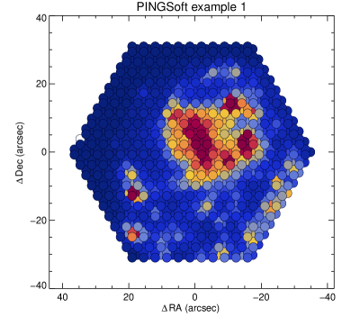
Figure 3: Postscript outputs examples of the view_3D routine

Examples:

To visualise the RSS file IRAS06295.VIMOS.fits with position table named IRAS06295.VIMOS.pt.txt (both included in pingsoft_examples/) limiting the intensity and wavelength range on the spectral window, drawing two vertical lines at lambda 6200 and 6700, using an inverse hyperbolic sine function scaling:

view_3d, ’IRAS06295.VIMOS.fits’,  min=-1, max=10, lmin=6200, lmax=6800, vline=[6200,6700], /asinh

To create a Postscript image of the ngc4625.dither.fits RSS file, with the spaxels drawn, the PINGSoft-special colour table, a 2% clipping scaling, using a narrow-band H$\alpha$ 20 Å filter, and a special title (shown in Figure 3):

view_3d, ’ngc4625.dither.fits’, ct=44, filter=2, /clip, /draw, /ps, _extra={title:’PINGSoft example 1’}

To create a Postscript image of IRAS06295.VIMOS.fits, with rainbow colour table, and using a B-Johnson (1965) filter and a special title (shown in Figure 3):

view_3d, ’IRAS06295.VIMOS.fits’, ct=33,  filter=3, /ps, _extra={title:’PINGSoft example 2’}

The following routines are introduced in the PINGSoft documentation.

Spectra extraction

extract_region: Extracts the spectra of regions selected by hand.

extract_aperture: Extracts the spectra within an elliptical or circular aperture.

extract_radial: Extracts radial average spectra within consecutive elliptical rings from a reference point, based on either fixed bins or S/N floor.

extract_slit: Extracts the spectra within a rectangular aperture, resembling a long-slit observation.

extract_cone: Extracts the spectra within a region defined by a hyperbolic cone.

extract_mask: Extracts the spectra based on a user’s given mask or segmentation map.

Data products and analysis

extract_filter: Generates a FITS image after convolving the 3D data with a narrow or broad-band filter.

s2n_ratio_3D: Extracts spectra interactively based on a continuum and emission line S/N floor.

s2n_optimize: Extracts spectra interactively based on a S/N optimization.

vfield_3D: Calculates the intrinsic velocity field in 3D data using a wavelength cross-correlation.

voronoi_3D: Applies a Voronoi tessallation to the IFS data using the Voronoi binning method by Cappellari & Copin (2003), MNRAS, 342, 345

IFS manipulation

split_califa: Extracts the FITS extensions for the CALIFA data.

read_rss: Reads a RSS FITS file and stores the data into an IDL vector.

merge_rss: Merges a list of RSS files into a single RSS file.

show_hdr: Shows on screen the header of a FITS file, which can be written to an ASCII file.

write_hdr: Adds or updates an entry in the header of a FITS file, using the fxaddpar.pro utility.

copy_hdr: Copies the header of one FITS file to another, USE WITH CAUTION!

cube2rss: Converts a 3D FITS cube with dimensions $X$, $Y$, $\lambda$ to a RSS FITS file plus an ad hoc position table in ASCII format.

Miscellaneous routines

write_wcs: Adds or updates the WCS (World Coordinate Systems) entries in a FITS header.

get_new_pt: Generates a new position table based on an index of selected spaxels.

shift_ptable: Shifts the reference point or applies an offset to a given position table.

merge_ptable: Concatenates a list of position table files into a single one for mosaicking purposes.

offset2radec: Transforms small angle offsets in arcsec from a reference point to equatorial coordinates.

radec2offset: Transforms equatorial coordinates to small angle offsets from a given reference point.

References

- Cappellari & Copin (2003) Cappellari M., Copin Y., 2003, MNRAS, 342, 345
- Rosales-Ortega (2011) Rosales-Ortega F. F., 2011, NewA, 16, 220
IMPORTANT:
If you find this code useful for your research please acknowledge
the use of PINGSoft in your publications:
Rosales-Ortega (2011) NewAstron 16, 220
Bugs, errors and inconsistencies (especially with non-tested
instruments) are expected. If you want to report a bug, or if you have any
comments or suggestions please contact the author at: frosales@inaoep.mx
Copyright © 2010, 2012 F. Fabián Rosales-Ortega
PINGSoft is licensed under GPLv3.
PINGSoft is free software: you can redistribute it and/or modify
it under the terms of the GNU General Public License as published by
the Free Software Foundation, version 3.
PINGSoft is distributed in the hope that it will be useful,
but WITHOUT ANY WARRANTY; without even the implied warranty of
MERCHANTABILITY or FITNESS FOR A PARTICULAR PURPOSE. See the
GNU General Public License for more details.
The GNU General Public License is found in: http://www.gnu.org/licenses/gpl.html