Numerical stability of relativistic beam multidimensional PIC simulations employing the Esirkepov algorithm

Abstract

Rapidly growing numerical instabilities routinely occur in multidimensional particle-in-cell computer simulations of plasma-based particle accelerators, astrophysical phenomena, and relativistic charged particle beams. Reducing instability growth to acceptable levels has necessitated higher resolution grids, high-order field solvers, current filtering, etc. except for certain ratios of the time step to the axial cell size, for which numerical growth rates and saturation levels are reduced substantially. This paper derives and solves the cold beam dispersion relation for numerical instabilities in multidimensional, relativistic, electromagnetic particle–in-cell programs employing either the standard or the Cole-Karkkainnen finite difference field solver on a staggered mesh and the common Esirkepov current-gathering algorithm. Good overall agreement is achieved with previously reported results of the WARP code. In particular, the existence of select time steps for which instabilities are minimized is explained. Additionally, an alternative field interpolation algorithm is proposed for which instabilities are almost completely eliminated for a particular time step in ultra-relativistic simulations.

1 Introduction

In a laser plasma accelerator (LPA), a laser pulse is propagated through a plasma, creating a wake of very strong electric fields of alternating polarity [1]. An electron beam injected with the appropriate phase can thus be accelerated to high energy in a distance much shorter than those for conventional acceleration techniques [2]. Simulation of a LPA stage from first principles using the Particle-In-Cell (PIC) technique in the laboratory frame is very demanding computationally, as the evolution of micron-scale laser oscillations needs to be followed over millions of time steps as the laser pulse propagates through a meter-long plasma for a 10 GeV stage [3].

A method recently was demonstrated to speed up full PIC simulations of a certain class of relativistic interactions by performing the calculation in a Lorentz boosted frame [4], taking advantage of the properties of space-time contraction and dilation in special relativity to render space and time scales (which are separated by orders of magnitude in the laboratory frame) comparable in a Lorentz boosted frame, resulting in far fewer computer operations. In the laboratory frame the laser pulse is much shorter than the wake, whose wavelength is also much shorter than the acceleration distance ($\lambda_{laser}\ll\lambda_{wake}\ll\lambda_{acceleration}$). In a Lorentz boosted frame co-propagating with the laser at a speed near the speed of light, the laser is Lorentz expanded (by a factor $\left(1+v_{f}\right)\gamma_{f}$, where $\gamma_{f}=\left(1-v_{f}^{2}\right)^{-1/2}$, $v_{f}$ is the velocity of the frame, normalized to the speed of light). The plasma (now moving opposite to the incoming laser at velocity $-v_{f}$) is Lorentz contracted by a factor $\gamma_{f}$. In a boosted frame moving with the wake (i.e., $\gamma_{f}\approx\gamma_{wake})$, the laser wavelength, the wake, and the acceleration length are comparable ($\lambda_{laser}<\lambda_{wake}\approx\lambda_{acceleration}$), leading to far fewer time steps by a factor $\left(1+v_{f}\right)^{2}\gamma_{f}^{2}$, hence far fewer computer operations [4, 5].

A violent numerical instability, associated with the plasma back-streaming at relativistic velocity $-v_{f}$ in the computational frame, limited early attempts to apply this method to speedups ranging between two and three orders of magnitude [3, 6, 7]. Control of the instability was obtained via the combination of: (i) the use of a tunable electromagnetic solver and an efficient wide-band digital filtering method [8], (ii) observation of the benefits of hyperbolic rotation of space-time on the laser spectrum in boosted frame simulations [9], and (iii) identification of a special time step at which the growth rate of the instability is greatly reduced [8]. The combination of these methods enabled the demonstration of speedups of over a million times [9]. The instability is described in some detail in [8].

In this paper, the analysis first reported in [10], which introduced the concept of numerical Cherenkov instabilities, is generalized and extended to two dimensions. (Extension to three dimensions follows readily from the analysis presented below, and the same conclusions apply.) The new analysis recovers the salient features of the instability described in [8], including the existence of the special time step. Growth rates are calculated for various cases of ultra-relativistic drifting plasmas and shown to match closely the growth rates obtained using the PIC code WARP [11]. Additionally, an alternative field interpolation algorithm is proposed for which instabilities are almost completely eliminated for a particular time step. A similar type of instability was reported in the calculation of astrophysical shocks [12], and the conclusions from this paper should apply readily.

A general derivation of the numerical instability dispersion relation for multidimensional PIC codes employing the Esirkepov algorithm is outlined in Sec. 2. The dispersion relation is specialized in Sec. 3 to a cold, relativistic beam in two dimensions for comparison with WARP simulations. Sec. 4 provides a simple yet reasonably accurate analytical expression for maximum numerical instability growth rates and, thereby, identifies time steps for which growth rates are significantly reduced, or even eliminated under some conditions. Then, the dispersion relation is solved numerically for a range of parameters and compared with WARP results in Sec. 5. (Most of these analytical and numerical calculations were performed using Mathematica [13]). Finally, Sec. 6 presents WARP simulations, demonstrating the near absence of numerical instabilities for an appropriately chosen field interpolation scheme and time step in two and three dimensions.

2 Numerical instability dispersion relation

The derivation here follows closely that of the general numerical instability dispersion relation in [14], and only those steps that differ will be presented . To start, the present derivation is based on the electromagnetic fields themselves rather than on the potentials.

$$\frac{\partial\mathbf{E}}{\partial t}=\nabla\times\mathbf{B}-\mathbf{J\mathrm{,}}$$ (1)

$$\frac{\partial\mathbf{B}}{\partial t}=-\nabla\times\mathbf{E\mathrm{.}}$$ (2)

Units are chosen such that, without loss of generality, the speed of light and other constants are unity. If the differential equations are replaced by corresponding finite difference equations, and the difference equations Fourier-transformed in space and time, we obtain expressions of the form,

$$[\omega]\mathbf{E=-[k]}\times\mathbf{B}+i\mathbf{J\mathrm{,}}$$ (3)

$$[\omega]\mathbf{B=[k]}\times\mathbf{E\mathrm{.}}$$ (4)

Brackets around quantities designate their finite difference representations.

The Esirkepov algorithm determines not the current itself but its first derivative; see Eq. (19) of [15]. The Fourier transform of this equation can be written as,

$$\left\{\begin{array}[]{c}W_{x}\\ W_{y}\\ W_{z}\end{array}\right\}=-i\Delta t\left\{\begin{array}[]{c}[k_{x}]\mathscr{\mathcal{J}}_{x}\\ {}[k_{y}]\mathcal{J}_{y}\\ {}[k_{z}]\mathcal{J}_{z}\end{array}\right\},$$ (5)

with $\boldsymbol{\mathcal{J}}$ the current contribution of an individual particle, and $\Delta t$ the simulation time step. $\mathbf{W}$ is further defined in terms of the current interpolation function $S^{J}$ by Eq. (23) of [15], which when Fourier-transformed becomes,

$$\left\{\begin{array}[]{c}W_{x}\\ W_{y}\\ W_{z}\end{array}\right\}=-2iS^{J}\left\{\begin{array}[]{c}\sin\left(k_{x}^{\prime}v_{x}\frac{\Delta t}{2}\right)\left[\cos\left(k_{y}^{\prime}v_{y}\frac{\Delta t}{2}\right)\cos\left(k_{z}^{\prime}v_{z}\frac{\Delta t}{2}\right)-\frac{1}{3}\sin\left(k_{y}^{\prime}v_{y}\frac{\Delta t}{2}\right)\sin\left(k_{z}^{\prime}v_{z}\frac{\Delta t}{2}\right)\right]\\ \sin\left(k_{y}^{\prime}v_{y}\frac{\Delta t}{2}\right)\left[\cos\left(k_{z}^{\prime}v_{z}\frac{\Delta t}{2}\right)\cos\left(k_{x}^{\prime}v_{x}\frac{\Delta t}{2}\right)-\frac{1}{3}\sin\left(k_{z}^{\prime}v_{z}\frac{\Delta t}{2}\right)\sin\left(k_{x}^{\prime}v_{x}\frac{\Delta t}{2}\right)\right]\\ \sin\left(k_{z}^{\prime}v_{z}\frac{\Delta t}{2}\right)\left[\cos\left(k_{x}^{\prime}x_{y}\frac{\Delta t}{2}\right)\cos\left(k_{y}^{\prime}v_{y}\frac{\Delta t}{2}\right)-\frac{1}{3}\sin\left(k_{x}^{\prime}v_{x}\frac{\Delta t}{2}\right)\sin\left(k_{y}^{\prime}v_{y}\frac{\Delta t}{2}\right)\right]\end{array}\right\},$$ (6)

with $\mathbf{v}$ the particle velocity. Combining Eqs. (5) and (6) provides the desired expression for the particle current,

$$\left\{\begin{array}[]{c}\mathcal{J}_{x}\\ \mathcal{J}_{y}\\ \mathcal{J}_{z}\end{array}\right\}=S^{J}\frac{2}{\Delta t}\left\{\begin{array}[]{c}\sin\left(k_{x}^{\prime}v_{x}\frac{\Delta t}{2}\right)\left[\cos\left(k_{y}^{\prime}v_{y}\frac{\Delta t}{2}\right)\cos\left(k_{z}^{\prime}v_{z}\frac{\Delta t}{2}\right)-\frac{1}{3}\sin\left(k_{y}^{\prime}v_{y}\frac{\Delta t}{2}\right)\sin\left(k_{z}^{\prime}v_{z}\frac{\Delta t}{2}\right)\right]/[k_{x}]\\ \sin\left(k_{y}^{\prime}v_{y}\frac{\Delta t}{2}\right)\left[\cos\left(k_{z}^{\prime}v_{z}\frac{\Delta t}{2}\right)\cos\left(k_{x}^{\prime}v_{x}\frac{\Delta t}{2}\right)-\frac{1}{3}\sin\left(k_{z}^{\prime}v_{z}\frac{\Delta t}{2}\right)\sin\left(k_{x}^{\prime}v_{x}\frac{\Delta t}{2}\right)\right]/[k_{y}]\\ \sin\left(k_{z}^{\prime}v_{z}\frac{\Delta t}{2}\right)\left[\cos\left(k_{x}^{\prime}x_{y}\frac{\Delta t}{2}\right)\cos\left(k_{y}^{\prime}v_{y}\frac{\Delta t}{2}\right)-\frac{1}{3}\sin\left(k_{x}^{\prime}v_{x}\frac{\Delta t}{2}\right)\sin\left(k_{y}^{\prime}v_{y}\frac{\Delta t}{2}\right)\right]/[k_{z}]\end{array}\right\}.$$ (7)

This expression must, of course, be integrated over the linearized particle distribution function to obtain the total current. Note that Eq. (7) reduces to $\boldsymbol{\mathcal{J}}=\mathit{\mathbf{v}}$ in the limit of vanishing time step and cell size, as it should.

Modeling relativistic simulations requires replacing $d\mathbf{v}/dt$ by $d\mathbf{p}/dt$, with $\mathbf{p=\gamma\mathbf{v}}$ the relativistic momentum and $\gamma$ the relativistic energy, in Eq. (16) of [14]. This change flows through to Eqs. (17) and (18), in which

$$\frac{\partial}{\partial\mathbf{p}}=\frac{1}{\gamma}\frac{\partial}{\partial\mathbf{v}}-\frac{\mathbf{p}}{\gamma^{3}}\mathbf{p\cdot\frac{\partial}{\partial\mathbf{v}}}$$ (8)

replaces $\partial/\partial\mathbf{v}$. The force in Eqs. (17) - (19) of [14] applied to the particles is $\mathbf{E}+\mathbf{v}$$\times\mathbf{B}$, with the components of $\mathbf{E}$ and $\mathbf{B}$ multiplied by the Fourier transforms of their respective interpolations functions:

$$\left\{\begin{array}[]{c}F_{x}\\ F_{y}\\ F_{z}\end{array}\right\}=\left\{\begin{array}[]{c}S^{E_{x}}E_{x}+v_{y}S^{B_{z}}B_{z}-v_{z}S^{B_{y}}B_{y}\\ S^{E_{y}}E_{y}+v_{z}S^{B_{x}}B_{x}-v_{x}S^{B_{z}}B_{z}\\ S^{E_{z}}E_{z}+v_{x}S^{B_{y}}B_{y}-v_{y}S^{B_{x}}B_{x}\end{array}\right\}.$$ (9)

In contrast to [14], the Fourier-transformed field interpolation functions are not assumed to be identical.

Replacing appropriate parts of Eqs. (18) and (23) of [14] by the corresponding terms from Eqs. (7) - (9) yields

$$\mathbf{J}=\sum_{m}\int\mathbf{F\cdot\frac{\partial}{\partial\mathbf{p}}\,\mathcal{\boldsymbol{J}}\,\csc}\left[\left(\omega-\mathbf{k^{\prime}\cdot v}\right)\frac{\Delta t}{2}\right]\frac{\Delta t}{2}f\,\mathrm{d}^{3}\mathbf{v}$$ (10)

summed over spatial aliases $m_{z}$ and $m_{x}$, as defined in [14]. The determinant of the 6x6 matrix comprised of Eqs. (3), (4), and (10) is the desired dispersion relation. A striking difference between this and the general dispersion relation in [14] is that the present dispersion relation contains trigonometric functions involving particle velocities.

3 WARP 2-d dispersion relation

For comparison with WARP two-dimensional, cold beam simulation results [8], we reduce Eqs. (3) and (4) to a 3x3 system in $\left\{E_{z},E_{x},B_{y}\right\}$ and perform the integral in Eq(10) for a cold beam propagating at velocity v in the z-direction. The resulting matrix equation is

$$\left(\begin{array}[]{ccc}\xi_{z,z}+[\omega]&\xi_{z,x}&\xi_{z,y}+[k_{x}]\\ 0&\xi_{x,x}+[\omega]&\xi_{x,y}-[k_{z}]\\ D_{x}^{*}[k_{x}]&-D_{z}^{*}[k_{z}]&[\omega]\end{array}\right)\left(\begin{array}[]{c}E_{z}\\ E_{x}\\ B_{y}\end{array}\right)=0.$$ (11)

$D_{z}^{*}$ and $D_{x}^{*}$ are introduced at this point to accommodate the Cole-Karkkainnen field solver, sometimes used in WARP; it is discussed near the end of this section. The quantities $\xi$ are employed purely for notational simplicity.

$$\xi_{z,z}\equiv-n\gamma^{-2}\sum_{m}S^{J}S^{E_{z}}\csc^{2}\left[\left(\omega-k_{z}^{\prime}v\right)\frac{\Delta t}{2}\right]\frac{\Delta t}{2}\sin\left(\omega\frac{\Delta t}{2}\right)k_{z}^{\prime}/[k_{z}]\mathrm{,}$$ (12)

$$\xi_{z,x}\equiv-n\sum_{m}S^{J}S^{E_{x}}\csc\left[\left(\omega-k_{z}^{\prime}v\right)\frac{\Delta t}{2}\right]\cot\left[\left(\omega-k_{z}^{\prime}v\right)\frac{\Delta t}{2}\right]\frac{\Delta t}{2}\sin\left(k_{z}^{\prime}v\frac{\Delta t}{2}\right)k_{x}^{\prime}/[k_{z}],$$ (13)

$$\xi_{z,y}\equiv nv\sum_{m}S^{J}S^{B_{y}}\csc\left[\left(\omega-k_{z}^{\prime}v\right)\frac{\Delta t}{2}\right]\cot\left[\left(\omega-k_{z}^{\prime}v\right)\frac{\Delta t}{2}\right]\frac{\Delta t}{2}\sin\left(k_{z}^{\prime}v\frac{\Delta t}{2}\right)k_{x}^{\prime}/[k_{z}],$$ (14)

$$\xi_{x,x}\equiv-n\sum_{m}S^{J}S^{E_{x}}\csc\left[\left(\omega-k_{z}^{\prime}v\right)\frac{\Delta t}{2}\right]\frac{\Delta t}{2}\cos\left(k_{z}^{\prime}v\frac{\Delta t}{2}\right)k_{x}^{\prime}/[k_{x}],$$ (15)

$$\xi_{x,y}\equiv nv\sum_{m}S^{J}S^{B_{y}}\csc\left[\left(\omega-k_{z}^{\prime}v\right)\frac{\Delta t}{2}\right]\frac{\Delta t}{2}\cos\left(k_{z}^{\prime}v\frac{\Delta t}{2}\right)k_{x}^{\prime}/[k_{x}].$$ (16)

summed over spatial aliases, $k_{z}^{\prime}=k_{z}+m_{z}\,2\pi/\Delta z$ and $k_{x}^{\prime}=k_{x}+m_{x}\,2\pi/\Delta x$, with $m_{z}$ and $m_{x}$ integers. The resonances, $\omega-k_{z}^{\prime}v$, introduce an infinity of spurious beam modes with effective charge densities proportional to $S^{J}S^{E_{z}}$, etc. n is the beam charge density divided by $\gamma$, which can be normalized to unity. However, explicitly retaining it in the dispersion relation sometimes is informative.

WARP employs the usual staggered spatial mesh and E-B leapfrog in time [16]. Hence,

$$\left[\omega\right]=\sin\left(\omega\frac{\Delta t}{2}\right)/\left(\frac{\Delta t}{2}\right),$$ (17)

$$\left[k_{z}\right]=\sin\left(k_{z}\frac{\Delta z}{2}\right)/\left(\frac{\Delta z}{2}\right),$$ (18)

$$\left[k_{x}\right]=\sin\left(k_{x}\frac{\Delta x}{2}\right)/\left(\frac{\Delta x}{2}\right).$$ (19)

Also as usual, WARP employs splines for current and field interpolation. The Fourier transform of the current interpolation function is

$$S^{J}=\left[\sin\left(k_{z}^{\prime}\frac{\Delta z}{2}\right)/\left(k_{z}^{\prime}\frac{\Delta z}{2}\right)\right]^{\ell_{z}+1}\left[\sin\left(k_{x}^{\prime}\frac{\Delta x}{2}\right)/\left(k_{x}^{\prime}\frac{\Delta x}{2}\right)\right]^{\ell_{x}+1},$$ (20)

$\ell_{z}$ and $\ell_{x}$ are the orders of the current interpolation splines in the z- and x-directions. So, for instance, an exponent of 2 in Eq. (20) corresponds to linear interpolation, and of 4 to cubic interpolation. Analogous definitions apply to the three field interpolation functions, but the spline orders need not be the same. WARP typically employs field interpolation splines like those of the currents but with the $E_{z}$ splines one order lower in z, the $E_{x}$ splines one order lower in x, and the $B_{y}$ splines one order lower in both. (This particular choice of spline orders is derivable by Galerkin’s method [17] and has superior energy conservation properties [18, 19, 20]. It will be referred to subsequently as “Galerkin field interpolation”.)

$$S^{E_{z}}=\left[\sin\left(k_{z}^{\prime}\frac{\Delta z}{2}\right)/\left(k_{z}^{\prime}\frac{\Delta z}{2}\right)\right]^{\ell_{z}}\left[\sin\left(k_{x}^{\prime}\frac{\Delta x}{2}\right)/\left(k_{x}^{\prime}\frac{\Delta x}{2}\right)\right]^{\ell_{x}+1}\left(-1\right)^{m_{z}},$$ (21)

$$S^{E_{x}}=\left[\sin\left(k_{z}^{\prime}\frac{\Delta z}{2}\right)/\left(k_{z}^{\prime}\frac{\Delta z}{2}\right)\right]^{\ell_{z}+1}\left[\sin\left(k_{x}^{\prime}\frac{\Delta x}{2}\right)/\left(k_{x}^{\prime}\frac{\Delta x}{2}\right)\right]^{\ell_{x}}\left(-1\right)^{m_{x}},$$ (22)

$$S^{B_{y}}=\cos\left(\omega\frac{\Delta t}{2}\right)\left[\sin\left(k_{z}^{\prime}\frac{\Delta z}{2}\right)/\left(k_{z}^{\prime}\frac{\Delta z}{2}\right)\right]^{\ell_{z}}\left[\sin\left(k_{x}^{\prime}\frac{\Delta x}{2}\right)/\left(k_{x}^{\prime}\frac{\Delta x}{2}\right)\right]^{\ell_{x}}\left(-1\right)^{m_{z}+m_{x}}.$$ (23)

The alias phase factors appearing at the ends of Eqs. (21) - (23) arise from the half-cell offsets from the current interpolation mesh of the corresponding fields. Averaging $B_{y}$ in time before applying it to particles causes the factor $\cos\left(\omega\frac{\Delta t}{2}\right)$ in Eq.(23).

Another credible choice of field interpolation functions is splines of the same order as those for the current interpolation function, in which case Eqs. (21) - (23) contain only powers of $\ell_{x}+1$ and $\ell_{z}+1$. The powers of -1 are unchanged. This seemingly minor change has a significant impact on numerical stability for some choices of $\Delta t$. (It will be referred to subsequently as “uniform field interpolation”.)

The Cole-Karkkainnen field solver [21, 22, 23], mentioned above, increases the Courant limit on the simulation time step and in some cases reduces numerical dispersion in the electromagnetic fields. It is discussed in some detail in Sec. 2.2 of [8]. For our purposes,

$$D_{z}^{*}=1-4\beta_{x}\sin^{2}\left(k_{x}\frac{\Delta x}{2}\right),$$ (24)

$$D_{x}^{*}=1-4\beta_{z}\sin^{2}\left(k_{z}\frac{\Delta z}{2}\right).$$ (25)

For $\Delta x=\Delta z$, the choice $\beta_{x}=\beta_{z}=1/8$ relaxes the Courant limit to $\Delta t<\Delta z$, while minimizing numerical dispersion in the vacuum fields along major axes.

Finally, we note that $m_{x}$ alias terms in the dispersion relation can be summed explicitly by means of Eqs. (1.421.3) and (1.422.3) of [24] or derivatives thereof, once choices have been made for the interpolation functions. For example, the $k_{x}^{\prime}$-dependent terms in $\xi_{z,z}$ sum to

$$\sum_{m_{x}}\left[\sin\left(k_{x}^{\prime}\frac{\Delta x}{2}\right)/\left(k_{x}^{\prime}\frac{\Delta x}{2}\right)\right]^{4}=\left[2\cos\left(k_{x}\frac{\Delta x}{2}\right)+1\right]/3$$ (26)

for $\ell_{x}=1$. Note that the $m_{x}=0$ term alone has the value $\left(2/\pi\right)^{4}$ for $k_{x}$ near its maximum value, $\pi/\Delta x$. In contrast, the sum has the value $\nicefrac{{1}}{{3}}$ there. (Most of the difference is due to the $m_{x}=-1$ alias, which is typical.) Since, as we shall see, peak growth rates typically scale as the cube root of such sums, the difference in predicted peak growth rates is of order 20%.

4 Approximate peak growth rates

$\xi_{z,z}$, defined in Eq. (12), scales as $\gamma^{-2}$ (with n held constant) and can be ignored for highly relativistic calculations, on which this paper focuses. Likewise, $1-v\simeq\gamma^{-2}/2$, and can be set to zero. Additionally,

$$\xi_{z,x}\xi_{x,y}-\xi_{z,y}\xi_{z,y}=0$$ (27)

is satisfied for individual modes and is satisfied approximately for cross-products between modes. With these assumptions the dispersion relation (the determinant of Eq. (11)) has the form

$$C_{0}+n\sum_{m_{z}}C_{1}\csc\left[\left(\omega-k_{z}^{\prime}\right)\frac{\Delta t}{2}\right]+n\sum_{m_{z}}C_{2}\csc^{2}\left[\left(\omega-k_{z}^{\prime}\right)\frac{\Delta t}{2}\right]=0.$$ (28)

with $C_{0}$ the vacuum dispersion function,

$$C_{0}=\left[\omega\right]^{2}-D_{z}^{*}\left[k_{x}\right]^{2}-D_{x}^{*}\left[k_{z}\right]^{2},$$ (29)

and

$$C_{1}=-\frac{C_{0}}{\left[\omega\right]}\frac{\Delta t}{2}\sum_{m_{x}}\frac{k_{x}^{\prime}}{\left[k_{x}\right]}S^{J}S^{E_{x}}\cos\left(k_{z}^{\prime}\frac{\Delta t}{2}\right)-D_{z}^{*}\frac{[k_{z}]^{2}}{\left[k_{x}\right]}\frac{\Delta t}{2}\sum_{m_{x}}k_{x}^{\prime}S^{J}\left(\frac{S^{E_{x}}}{\left[\omega\right]}-\frac{S^{B_{y}}}{[k_{z}]}\right)\cos\left(k_{z}^{\prime}\frac{\Delta t}{2}\right),$$ (30)

$$C_{2}=D_{x}^{*}[k_{x}]\frac{\Delta t}{2}\sum_{m_{x}}k_{x}^{\prime}S^{J}\left(\frac{S^{E_{x}}}{\left[\omega\right]}-\frac{S^{B_{y}}}{[k_{z}]}\right)\cos\left[\left(\omega-k_{z}^{\prime}\right)\frac{\Delta t}{2}\right]\sin\left(k_{z}^{\prime}\frac{\Delta t}{2}\right).$$ (31)

Eq.(28) reduces, of course, to $C_{0}+n=0$ in the limit of vanishing time step and cell size. All the beam modes in Eq.(28) are numerical artifacts, even the $m_{z}=0$ mode.

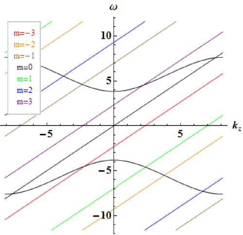
Figure 1: Normal mode diagram for$\frac{\Delta t}{\Delta z}=0.7$, $\beta=0$, and $k_{x}=\nicefrac{{1}}{{2}}\,\frac{\pi}{\Delta x}$, showing numerically distorted electromagnetic modes and spurious beam modes, $m_{z}=\left[-3,\,3\right]$. Numerical Cherenkov instabilities occur near mode intersections.

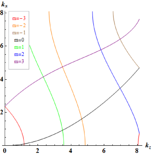
Figure 2: Locations in k-space of resonances between electromagnetic modes and beam modes, $m_{z}=\left[-3,\,3\right]$ for $\frac{\Delta t}{\Delta z}=0.7$ and $\beta=0$. Intersecting resonance curves occur at different frequencies and, therefore, do not interact.

Coupling between these beam numerical modes and electromagnetic modes (the roots of $C_{0}=0$) gives rise to what has become known as the numerical Cherenkov instability [10, 25], which can be quite virulent. Fig. 1 is a typical normal mode diagram, showing the two electromagnetic modes and beam aliases $m_{z}=$ [-3, 3] for $\Delta t=0.7\Delta z$, $\beta_{x}=\beta_{z}=0$, and $k_{x}=\nicefrac{{1}}{{2}}\,\frac{\pi}{\Delta x}$. (Unless otherwise noted, other parameters for this and other figures are $n=1$ and $\Delta x=\Delta z=0.3868$.) Fig. 2 depicts the locations in k-space of normal mode intersections, such as those in Fig. 1, as $k_{x}$ is varied.

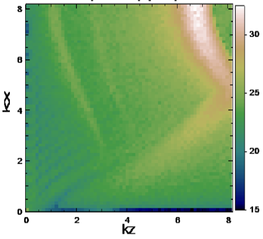
Figure 3: Fourier-transformed $E_{z}$ (log scale) at $t=16$ from a WARP simulation with Galerkin field interpolation, $\frac{\Delta t}{\Delta z}=0.7$, and $\beta=0$.

Comparing Fig. 2 with corresponding WARP results in Fig. 3 indicates that the strongest instabilities lie along the $m_{z}$= -1 and 0 resonance curves at larger $k_{x}$. (The WARP simulations were performed on a $128\times 128$ square grid with periodic boundary conditions and a uniformly distributed plasma moving axially at an energy of $\gamma=130$, seeded with a small random transverse velocity. Plots similar to Fig. 3 appear in [26, 27].) Also visible, although just barely, are much more slowly growing instabilities along the $m_{z}$= +1 and $m_{z}$= -2 resonance curves. We now proceed to estimate these instability growth rates.

Resonance curves, such as those in Fig. 2, are given by Eq. (29) with $\omega$ replaced by $k_{z}^{\prime}$ , solved for $k_{x}$ as a function of $k_{z}^{\prime}$. (Recall that $\sin^{2}\left(k_{z}^{\prime}\frac{\Delta z}{2}\right)=\sin^{2}\left(k_{z}\frac{\Delta z}{2}\right)$.)

$$k_{x}^{r}=\frac{2}{\Delta x}\arcsin\left(\sqrt{\frac{\left(\frac{\Delta t}{\Delta z}\right)^{2}\sin^{2}\left(k_{z}^{\prime}\frac{\Delta t}{2}\right)-\left(\frac{\Delta x}{\Delta z}\right)^{2}\sin^{2}\left(k_{z}^{\prime}\frac{\Delta z}{2}\right)}{1-4\sin^{2}\left(k_{z}^{\prime}\frac{\Delta z}{2}\right)\left(\beta_{x}+\beta_{z}\left(\frac{\Delta x}{\Delta z}\right)^{2}\right)}}\right)$$ (32)

To obtain an estimate of the numerical instability growth rate along a resonance curve, we expand $C_{0}$ and the cosecants in Eq. (28) to first order in $\left(\omega-k_{z}^{\prime}\right)$, set $C_{1}=0$, and set $\omega=k_{z}^{\prime}$ in $C_{2}$. The resulting cubic equation has one unstable root,

$$Im\left(\omega\right)\simeq\frac{\sqrt{3}}{2}\sqrt[3]{\frac{n}{2}D_{x}^{*}[k_{x}]\sum_{m_{x}}k_{x}^{\prime}S^{J}\left|\frac{\frac{\Delta t}{2}S^{E_{x}}}{\sin\left(k_{z}^{\prime}\frac{\Delta t}{2}\right)}-\frac{\frac{\Delta z}{2}S^{B_{y}}}{\sin\left(k_{z}^{\prime}\frac{\Delta z}{2}\right)}\right|\csc\left(k_{z}^{\prime}\frac{\Delta t}{2}\right)},$$ (33)

evaluated at $k_{x}=k_{x}^{r}$. Although it may appear that Eq. (33) becomes singular when $k_{z}^{\prime}$ approaches zero, $k_{x}^{r}$ approaches zero there also, as $k_{z}^{\prime}$². Consequently, the growth rate vanishes in that limit.

For completeness, we note that instability also occurs off-resonance when $C_{0}C_{2}>C_{1}^{\,2}/4$, evaluated at $\omega\simeq k_{z}^{\prime}$ and arbitrary $k_{x}$. The resulting growth rate is

$$Im\left(\omega\right)\simeq\frac{\sqrt{C_{1}^{\,2}/4-C_{0}C_{2}}}{C_{0}}.$$ (34)

Although off-resonance growth is weaker than on-resonance, it often occurs at smaller $k_{z}$, where it may be more difficult to filter. (The residual instabilities after digital filtering discussed in the fourth paragraph of Sec. 5 are, for instance, of this sort.)

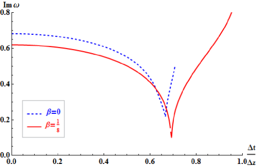
Figure 4: Approximate peak growth rate vs $\Delta t/\Delta z$ for Galerkin field interpolation with $\beta=0,\nicefrac{{1}}{{8}}$.

Fig. 4 displays maximum instability growth rates for the Galerkin field interpolation algorithm as $\Delta t/\Delta z$ varies over its range of allowed values for $\beta_{z}=\beta_{x}$ (collectively, $\beta)$ = 0 and $\nicefrac{{1}}{{8}}$. (Intermediate values of $\beta$ produce curves intermediate in shape.) The pronounced dip in both curves, at $\Delta t/\Delta z$$\approx 0.66$ for $\beta=0$ and 0.69 for $\beta=\nicefrac{{1}}{{8}}$, previously has been observed in simulations [8]. It occurs because $Im\left(\omega\right)$ vanishes for some value of $k_{z}$, which occurs when

$$\frac{\Delta t}{\Delta z}\sin^{2}\left(k_{z}^{\prime}\frac{\Delta z}{2}\right)=k_{z}^{\prime}\frac{\Delta z}{4}\sin\left(k_{z}^{\prime}\Delta t\right).$$ (35)

Eq. (35) has solutions for the $m_{z}$= -1 and 0 resonances only over a narrow range of time steps, $\sqrt{2}/2\geq\Delta t/\Delta z\gtrsim 0.65$. Precisely where the minimum falls within this range depends on algorithmic details.

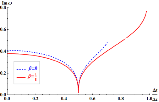
Figure 5: Approximate peak growth rate vs $\Delta t/\Delta z$ for uniform field interpolation with $\beta=0,\nicefrac{{1}}{{8}}$. The growth rate vanishes at $\Delta t=\Delta z/2$ for all values of $\beta$.

Similarly, Fig. 5 displays maximum instability growth rates for the uniform field interpolation algorithm as $\Delta t/\Delta z$ varies over its range of allowed values for $\beta$ = 0 and $\nicefrac{{1}}{{8}}$. For all values of $\beta$, the growth rate vanishes at $\Delta t/\Delta z$ = $\nicefrac{{1}}{{2}}$. Why this should be so is evident from

$$\frac{\Delta t}{\Delta z}\sin\left(k_{z}^{\prime}\frac{\Delta z}{2}\right)=\frac{1}{2}\sin\left(k_{z}^{\prime}\Delta t\right),$$ (36)

which differs from its Galerkin counterpart, Eq. (35), by a factor of $\sin\left(k_{z}^{\prime}\frac{\Delta z}{2}\right)/\left(k_{z}^{\prime}\frac{\Delta z}{2}\right)$. Eq. (36) is satisfied for all $k_{z}^{\prime}$ at $\Delta t/\Delta z$ = $\nicefrac{{1}}{{2}}$, and for no values (apart from 0) of $k_{z}^{\prime}$ otherwise.

Eq. (33) also provides a simple means for estimating the effect of current filtering on numerical Cherenkov instabilities, because the Fourier transform of the digital filtering function appears simply as a factor multiplying n. Given the substantial growth rates of this instability, filtering must reduce currents in regions of k-space where the instability is strong by some three orders of magnitude. Of course, any physical phenomena occurring in those same regions also will be suppressed. Using higher order interpolation (i.e., larger $\ell$’s in Eqs. (20) - (23)) also reduces numerical instability growth, especially for higher order aliases. However, for typical simulation parameters it reduces the $m_{z}$= -1 and 0 instability growth rates by comparable, modest factors. Employing cubic rather than linear splines, for instance, would be expected to reduce maximum growth rates by of order $\left(2/\pi\right)^{\nicefrac{{4}}{{3}}}$. On this basis current digital filtering usually is more cost effective than higher order interpolation for suppressing numerical Cherenkov instabilities.

5 Numerical solutions

Reliably finding the roots of Eq. (11) can be accomplished as follows. Given how strongly even linear interpolation suppresses all but the first few aliases, we safely can truncate the infinite series in $m_{z}$ to a range of, say, [-3, 3]. (Indeed, the smaller range [-1, 0] works fairly well in most cases.) Then, if the aliases are well separated in $\omega-k$ space (as they are in, for instance, Fig. 1), the growth rates for any particular alias can be evaluated with reasonable accuracy by expanding the dispersion relation as a fourth-order power series in $\left(\omega-k_{z}^{\prime}v\right)$ for the $k_{z}^{\prime}$ in question and calculating all roots with a polynomial root finder. On the other hand, if aliases are separated in frequency by only a few times the typical growth rates, the expansion converges slowly, and an iterative solution is required. The Mathematica [13] FindRoot routine was used for the results that follow in this section, with three real roots or one real root and one conjugate pair of roots found per alias. Evaluations were performed on a 65x65 array in k-space, consistent with the 128x128 spacial grid used in WARP for comparable simulations. Obtaining results for a typical set of parameters required about 15 minutes on a 2.8 GHz, 2 processor desktop computer.

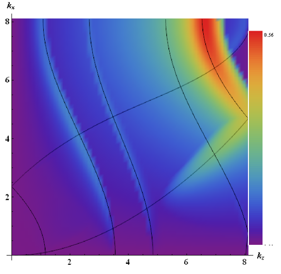
Figure 6: Instability growth rates calculated from the numerical dispersion relation for Galerkin field interpolation, $\frac{\Delta t}{\Delta z}=0.7$, and $\beta=0$. Fig. 3 shows corresponding WARP results. Resonance curves are as in Fig. 2.

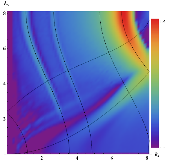
Figure 7: Instability growth rates for Galerkin field interpolation, $\frac{\Delta t}{\Delta z}=0.7$, and $\beta=0$, computed from WARP simulations characterized by Fig. 3

Fig. 6 presents numerical growth rate predictions corresponding to the WARP results in Fig. 3. The $m_{z}$= -1 alias dominates the growth spectrum with a maximum growth rate of 0.56 at short wavelengths in x. (The approximate growth rate based on the analysis in the previous section is 0.48.) Also visible is the fast growing $m_{z}$= 0 alias. The much weaker $m_{z}$= -2 and +1 aliases are evident at smaller $k_{z}$. As noted in the previous section, the $m_{z}$= -1, 0, and +1 aliases all can be seen in Fig. 3, although the last of these aliases is faint, consistent with its relatively slow growth. Fig. 7 depicts grow rates measured in this WARP simulation (actually the average of one hundred such simulations). The agreement between Figs. 6 and 7 is very good, especially when one considers the difficulty in measuring smaller growth rates in simulations, where nonlinear mode coupling and thermal noise can be significant. Thus, the method used to determine automatically the growth rates in WARP works well for the largest growth rates, which are of most interest in any particular simulation, but not so well for the smallest growth rates.

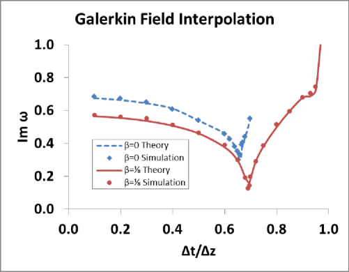
Figure 8: Maximum numerical instability growth rates observed in WARP and calculated from the numerical dispersion relation for Galerkin field interpolation with $\beta=0,\nicefrac{{1}}{{8}}$.

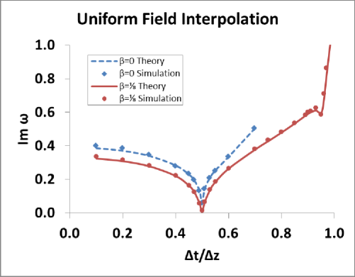
Figure 9: Maximum numerical instability growth rates observed in WARP and calculated from the numerical dispersion relation for uniform field interpolation with $\beta=0,\nicefrac{{1}}{{8}}$.

Maximum numerical growth rates observed in WARP for the Galerkin and uniform current interpolation algorithms with $\beta$=0 and $\nicefrac{{1}}{{8}}$ are compared with the predictions of linear theory in Figs. 8 and 9. Agreement between theory and simulation is very good. Qualitative agreement with the analytical estimates of the previous section is quite acceptable. The sudden rise of growth when $\Delta t/\Delta z$ nears unity for $\beta=\nicefrac{{1}}{{8}}$ comes from an instability of the field solver algorithm at the Nyquist limit and is mitigated by using one or more passes of bilinear filtering of the current density, as explained in Appendix A of [8] and shown below.

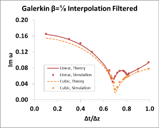
Figure 10: Maximum numerical instability growth rates observed in WARP and calculated from the numerical dispersion relation for digital filtering as described in Sec. 5, overall linear or cubic interpolation in z, and Galerkin field interpolation with $\beta=\nicefrac{{1}}{{8}}$.

Fig. 10 illustrates the effects of digital filtering and of higher order interpolation, in this case ten passes of the bilinear filter (including two compensation steps) described in [8], cubic or linear interpolation in z with Galerkin field gathering, and $\beta=\nicefrac{{1}}{{8}}$. The digital filter has the effect of multiplying n in the dispersion relation by

$$\cos^{16}\left(k_{z}\frac{\Delta z}{2}\right)\left(5-4\cos^{2}\left(k_{z}\frac{\Delta z}{2}\right)\right)^{2}\cos^{16}\left(k_{x}\frac{\Delta x}{2}\right)\left(5-4\cos^{2}\left(k_{x}\frac{\Delta x}{2}\right)\right)^{2}.$$ (37)

It effectively eliminates numerical instabilities for $k_{z}\Delta z/\pi\gtrsim 0.2$ or $k_{x}\Delta x/\pi\gtrsim 0.2$. With linear interpolation the $m_{z}=0$ alias dominates the numerical instabilty growth rate except in the vicinity of $\Delta t/\Delta z\approx 0.69$, where the $m_{z}=+1$ alias dominates. Growth rates are reduced by roughly a factor of four compared to those in Fig. 8. Cubic interpolation has negligible effect on the $m_{z}=0$ alias but almost completely suppresses the $m_{z}=+1$ alias. The minimum growth rate, now at $\Delta t/\Delta z\approx 0.70$, drops by a further factor of three. (Measuring the WARP instability growth rates for Fig. 10 was particularly challenging due to competition between the weak numerical instabilities, and thermal and nonlinear effects.)

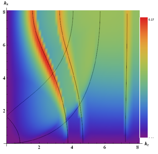
Figure 11: Instability growth rates calculated from the numerical dispersion relation with Galerkin field interpolation, $\frac{\Delta t}{\Delta z}=0.69$, and $\beta=\nicefrac{{1}}{{8}}$.

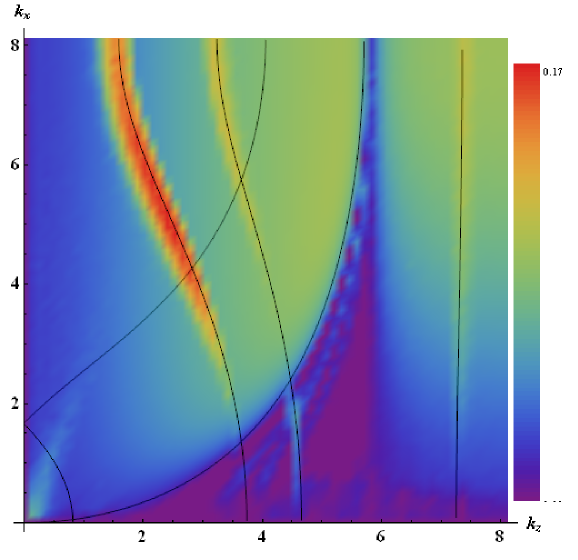
Figure 12: Instability growth rates observed in WARP simulations with Galerkin field interpolation, $\frac{\Delta t}{\Delta z}=0.69$, and $\beta=\nicefrac{{1}}{{8}}$.

As a further comparison between linear theory, Fig. 11, and WARP results, Fig.12 (also averaged over 100 simulations), we present growth rates for Galerkin current interpolation with $\frac{\Delta t}{\Delta z}=0.69$, and $\beta=\nicefrac{{1}}{{8}}$. The dominant alias is $m_{z}=+1$, occurring at the rather small axial wave numbers, $1.5<k_{z}<3.5$, and at most $k_{x}$ values away from the $k_{z}$-axis. Modestly to the right is the $m_{z}=-2$ alias, occurring at $3<k_{z}<4$ for large values of $k_{x}$. Generally, we expect the $m_{z}=+1$ and -2 aliases to have comparable growth rates, just as the $m_{z}=0$ and -1 aliases typically do. Finally, the $m_{z}=-3$ alias is modestly above background on the far right. For all these modes, theory and simulation growth rates agree to within about 15%. However, a region of reduced growth rate in the band $5<k_{z}<6$ occurs only in Fig. 12, although it can be produced in Fig. 11 by artificially removing the off-resonance $m_{z}=-1$ contribution. This minor discrepancy is apparent only for parameters very near those listed in this paragraph.

6 Application to the modeling of laser plasma acceleration

As a verification that the theory that has been developed in this paper applies to the modeling of LPAs, series of two and three dimensional simulations of a 100 MeV class LPA stage were performed, focusing on the plasma wake formation, using the parameters given in table 1. The velocity of the wake in the plasma corresponds to $\gamma\simeq 13.2$, and the simulations were performed in a boosted frame of $\gamma_{f}=13.$

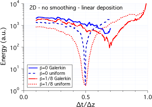
Figure 13: Field energy relative to stable reference level vs $\Delta t/\Delta z$ from two dimensional WARP LPA simulations at $\gamma$ = 13, using Galerkin and uniform field interpolation with $\beta=0,\nicefrac{{1}}{{8}}$, no filtering, and linear interpolation.

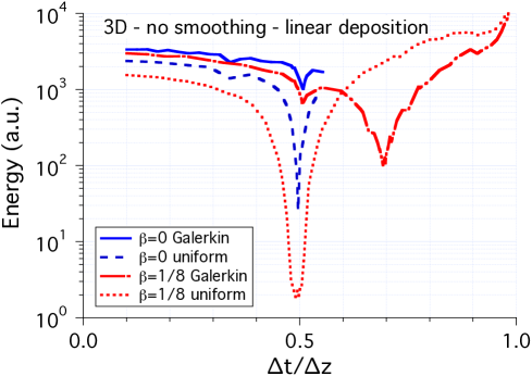
Figure 14: Field energy relative to stable reference level vs $\Delta t/\Delta z$ from three dimensional WARP LPA simulations at $\gamma$ = 13, using Galerkin and uniform field interpolation with $\beta=0,\nicefrac{{1}}{{8}}$.

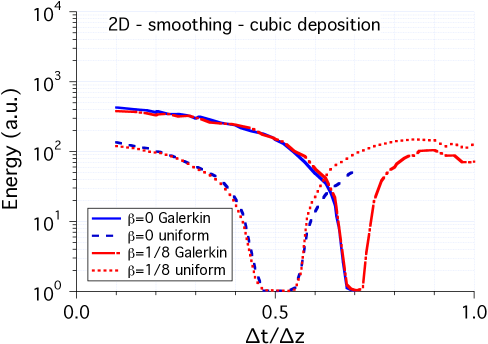
Figure 15: Field energy relative to stable reference level vs $\Delta t/\Delta z$ from three dimensional WARP LPA simulations at $\gamma$ = 13, using Galerkin and uniform field interpolation with $\beta=0,\nicefrac{{1}}{{8}}$.

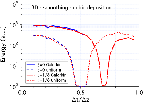
Figure 16: Field energy relative to stable reference level vs $\Delta t/\Delta z$ from three dimensional WARP LPA simulations at $\gamma$ = 13, using Galerkin and uniform field interpolation with $\beta=0,\nicefrac{{1}}{{8}}$.

Reference simulations were run in two and three dimensions for conditions where no instability developed, and the final total field energy $W_{f0}$ was recorded as a reference value in each case. Runs then were conducted for the Yee ($\beta=0$) and Cole-Karkkainnen ($\beta=1/8$) solvers, with Galerkin and uniform field interpolations. The final energy $W_{f}$ was recorded and divided by the reference energy $W_{f0}$. The ratio $W_{f}/W_{f0}$ is plotted versus time step from two dimensional simulations in Fig. 13 and from three dimensional simulations in Fig. 14, using linear current deposition and no smoothing of current and fields. Following the theoretical predictions, for the Galerkin interpolation scheme the instability is minimal around $\triangle t/\triangle z\approx 0.65$ when $\beta=0$ and around $\triangle t/\triangle z\approx 0.69$ when $\beta=1/8$, while for the uniform interpolation scheme the instability is minimal around $\triangle t/\triangle z\approx 0.5$. The ratio $W_{f}/W_{f0}$ also is plotted versus time step from two dimensional simulations in Fig. 15 and from three dimensional simulations in Fig. 16, using, as is common practice in the modeling of laser plasma stages, cubic current deposition and 1 pass of bilinear smoothing plus compensation of current and fields gathered onto macroparticles. The beneficial impact on stability of smoothing and high order deposition is evident from the relatively wide band of stability that is available around $\triangle t/\triangle z\approx 0.5$ with uniform gather, and the narrower band of stability that is available around $\triangle t/\triangle z\approx 0.7$ with Galerkin gather. This verifies that the theoretical results apply to real case simulations in two and three dimensions.

Table 1: List of parameters for a LPA stage simulation at 100 MeV

plasma density on axis	$n_{e}$	$10^{19}$ cm-3
plasma longitudinal profile		flat
plasma length	$L_{p}$	$1.5$ mm
plasma entrance ramp profile		half sine
plasma entrance ramp length		$20$ $\mu$m
laser profile		$a_{0}\exp\left(-r^{2}/2\sigma^{2}\right)\sin\left(\pi z/3L\right)$
normalized vector potential	$a_{0}$	$1$
laser wavelength	$\lambda$	$0.8$ $\mu$m
laser spot size (RMS)	$\sigma$	$8.91$ $\mu$m
laser length (HWHM)	$L$	$3.36$ $\mu$m
normalized laser spot size	$k_{p}\sigma$	$5.3$
normalized laser length	$k_{p}L$	$2$
cell size in x	$\Delta x$	$\lambda/32$
cell size in y (3D only)	$\Delta y$	$\lambda/32$
cell size in z	$\Delta z$	$\lambda/32$
# of plasma particles/cell		1 macro-e-+1 macro-p+

7 Conclusion

The numerical stability properties of multidimensional PIC codes employing the Esirkepov current algorithm have been derived. Just as in PIC codes employing earlier current algorithms, here also fast-growing numerical instabilities are predicted for relativistic beam simulations. These instabilities can, of course, be reduced significantly by short wavelength digital filtering. However, time steps have been identified at which instability growth is reduced even without filtering. Particularly noteworthy is uniform field interpolation with $\Delta t/\Delta z$ = $\nicefrac{{1}}{{2}}$ and any value of $\beta$, for which simulations are numerically stable in the large $\gamma$ limit. These results have been confirmed with the WARP simulation code.

Additionally, WARP LPA simulations performed using uniform field interpolation with $\Delta t/\Delta z$ = $\nicefrac{{1}}{{2}}$ have demonstrated the practical value of this choice of parameters in two and three dimensions. The uniform field interpolation offers much reduced growth rates, enabling faster simulations with fewer grid cells, lower order interpolation, and reduced digital filtering. In three dimensions, it enables existing PIC codes that incorporate the Yee solver, but not the CK solver, to benefit from the reduced growth rates at the special time steps over a wider range of cell aspect ratios (for cubic cells for example, the special time step is accessible only to the CK solver for Galerkin gather, while it is accessible to both the Yee and the CK solvers for uniform gather). The results that were obtained here also should apply readily to more efficient modeling of astrophysical shocks that use the same algorithms.

Finally, the salutary effect of trigonometric functions involving particle velocities in the dispersion relation of the Esirkepov algorithm suggest that further improvements in PIC code stability can be achieved by developing field interpolation algorithms that introduce similar trigonometric functions, perhaps along the lines of Sec. 4 in [14].

8 Acknowledgments

We wish to thank Irving Haber for suggesting this collaboration and for many helpful recommendations. We also are indebted to David Grote for support in using the code WARP at the National Energy Research Supercomputing Center and to Andrew Moylan for advice on using Mathematica to find arrays of roots to transcendental equations. This work was supported in part by the Director, Office of Science, Office of High Energy Physics, U.S. Dept. of Energy under Contract No. DE-AC02-05CH11231 and the US-DOE SciDAC ComPASS collaboration, and used resources of the National Energy Research Scientific Computing Center.

References

This document was prepared as an account of work sponsored in part by the United States Government. While this document is believed to contain correct information, neither the United States Government nor any agency thereof, nor The Regents of the University of California, nor any of their employees, nor the authors makes any warranty, express or implied, or assumes any legal responsibility for the accuracy, completeness, or usefulness of any information, apparatus, product, or process disclosed, or represents that its use would not infringe privately owned rights. Reference herein to any specific commercial product, process, or service by its trade name, trademark, manufacturer, or otherwise, does not necessarily constitute or imply its endorsement, recommendation, or favoring by the United States Government or any agency thereof, or The Regents of the University of California. The views and opinions of authors expressed herein do not necessarily state or reflect those of the United States Government or any agency thereof or The Regents of the University of California.

References

- [1] T. Tajima, J. Dawson, Laser electron-accelerator, Physical Review Letters 43 (4) (1979) 267–270.
- [2] W. P. Leemans, B. Nagler, A. J. Gonsalves, C. Toth, K. Nakamura, C. G. R. Geddes, E. Esarey, C. B. Schroeder, S. M. Hooker, Gev electron beams from a centimetre-scale accelerator, Nature Physics 2 (10) (2006) 696–699. doi:10.1038/nphys418.
- [3] D. Bruhwiler, J. Cary, B. Cowan, K. Paul, C. Geddes, P. Mullowney, P. Messmer, E. Esarey, E. Cormier-Michel, W. Leemans, J.-L. Vay, New developments in the simulation of advanced accelerator concepts, in: AIP Conference Proceedings, Vol. 1086, 2009, pp. 29–37.
- [4] J.-L. Vay, Noninvariance of space- and time-scale ranges under a lorentz transformation and the implications for the study of relativistic interactions, Physical Review Letters 98 (13) (2007) 130405/1–4.
- [5] J. L. Vay, C. G. R. Geddes, E. Esarey, C. B. Schroeder, W. P. Leemans, E. Cormier-Michel, D. P. Grote, Modeling of 10 GeV-1 TeV laser-plasma accelerators using Lorentz boosted simulations, Physics of Plasmas 18 (12). doi:{10.1063/1.3663841}.
- [6] J.-L. Vay, et al., Application of the reduction of scale range in a lorentz boosted frame to the numerical simulation of particle acceleration devices, in: Proc. Particle Accelerator Conference, Vancouver, Canada, 2009, tU1PBI04.
- [7] S. F. Martins, R. A. Fonseca, W. Lu, W. B. Mori, L. O. Silva, Exploring laser-wakefield-accelerator regimes for near-term lasers using particle-in-cell simulation in lorentz-boosted frames, Nature Physics 6 (4) (2010) 311–316. doi:10.1038/NPHYS1538.
- [8] J. L. Vay, C. G. R. Geddes, E. Cormier-Michel, D. P. Grote, Numerical methods for instability mitigation in the modeling of laser wakefield accelerators in a lorentz-boosted frame, Journal of Computational Physics 230 (15) (2011) 5908–5929. doi:10.1016/j.jcp.2011.04.003.
- [9] J. Vay, C. G. R. Geddes, E. Cormier-Michel, D. P. Grote, Effects of hyperbolic rotation in minkowski space on the modeling of plasma accelerators in a lorentz boosted frame, Physics of Plasmas 18 (3) (2011) 030701. doi:10.1063/1.3559483.
- [10] B. Godfrey, Numerical cherenkov instabilities in electromagnetic particle codes, Journal of Computational Physics 15 (4) (1974) 504–521.
- [11] D. Grote, A. Friedman, J.-L. Vay, I. Haber, The warp code: modeling high intensity ion beams, in: AIP Conference Proceedings, no. 749, 2005, pp. 55–8.
- [12] L. Sironi, A. Spitkovsky, private Communication (2011).
- [13] Mathematica, 8th Edition, Wolfram Research Inc., 2011.
- [14] B. Godfrey, Canonical momenta and numerical instabilities in particle codes, Journal of Computational Physics 19 (1) (1975) 58–76.
- [15] T. Esirkepov, Exact charge conservation scheme for particle-in-cell simulation with an arbitrary form-factor, Computer Physics Communications 135 (2) (2001) 144–153.
- [16] K. Yee, Numerical solution of initial boundary value problems involving maxwells equations in isotropic media, IEEE Transactions on Antennas and Propagation AP14 (3) (1966) 302–307.
- [17] B. Godfrey, L. Thode, Galerkin difference schemes for plasma simulation codes, Proc. Seventh Conf. Num. Sim. Plas., New York (1975) 87.
- [18] H. Lewis, Variational algorithms for numerical simulation of collisionless plasma with point particles including electromagnetic interactions, Journal of Computational Physics 10 (3) (1972) 400–419.
- [19] A. Langdon, Energy-conserving plasma simulation algorithms, Journal of Computational Physics 12 (2) (1973) 247–268.
- [20] C. Birdsall, A. Langdon, Plasma physics via computer simulation, Adam-Hilger, 1991.
- [21] J. Cole, A high-accuracy realization of the yee algorithm using non-standard finite differences, IEEE Transactions on Microwave Theory and Techniques 45 (6) (1997) 991–996.
- [22] J. Cole, High-accuracy yee algorithm based on nonstandard finite differences: New developments and verifications, IEEE Transactions on Antennas and Propagation 50 (9) (2002) 1185–1191. doi:10.1109/TAP.2002.801268.
- [23] M. Karkkainen, E. Gjonaj, T. Lau, T. Weiland, Low-dispersionwake field calculation tools, in: Proc. of International Computational Accelerator Physics Conference, Chamonix, France, 2006, pp. 35–40.
- [24] I. Gradshteyn, I. Ryzhik, Table of Integrals, Series, and Products, 3rd Edition, Academic Press, Inc., 1965.
- [25] B. Godfrey, Electromagnetic, strictly two-dimensional numerical instability in particle codes, Conference on Particle and Hybrid Codes in Fusion, Napa, California.
- [26] P. Yu, X. Xu, F. Tsung, W. Lu, V. K. Decyk, W. B. Mori, J. Vieira, R. A. Fonseca, L. O. Silva, Numerical instability due to relativistic plasma drift in EM-PIC code, American Institute of Physics, 2012.
- [27] J.-L. Vay, C. Benedetti, D. Bruhwiler, E. Cormier-Michel, B. Cowan, R. Fonseca, D. Gordon, A. Lifshitz, W. Mori, Efficient Particle-In-Cell algorithms for the modeling of advanced accelerators, American Institute of Physics, 2012.