Average-Atom Model for X-ray Scattering from Warm Dense Matter

Abstract

A scheme for analyzing Thomson scattering of x-rays by warm dense matter, based on the average-atom model, is developed. Emphasis is given to x-ray scattering by bound electrons. Contributions to the scattered x-ray spectrum from elastic scattering by electrons moving with the ions and from inelastic scattering by free and bound electrons are evaluated using parameters (chemical potential, average ionic charge, free electron density, bound and continuum wave functions, and occupation numbers) taken from the average-atom model. The resulting scheme provides a relatively simple diagnostic for use in connection with x-ray scattering measurements. Applications are given to dense hydrogen, beryllium, aluminum, titanium, and tin plasmas. At high momentum transfer, contributions from inelastic scattering by bound electrons are dominant features of the scattered x-ray spectrum for aluminum, titanium, and tin.

1 Introduction

Measurements of Thomson scattering of x-rays provide information on temperatures, densities and ionization balance in warm dense matter. Various techniques for inferring plasma properties from x-ray scattering measurements have been developed over the past decade GGL:02 ; LB:02 ; GG:03 ; LM:03 ; GGL:03 ; GGL:03a ; HR:04 ; GGL:06 ; GL:07 ; TB:08 ; KN:08 ; FT:09 ; DL:09 ; KG:09 ; GL:10 ; MM:10 ; TB:10 ; RR:10 ; KD:11 ; VD:12 ; FL:12 ; ZB:12 . Many of these techniques, together with the underlying theory, were reviewed by Glenzer and Redmer in Ref. GR:09 .

The present average-atom scheme is based on a theoretical description of x-ray scattering proposed by Gregori GG:03 , the important difference being that parameters used to evaluate the Thomson-scattering dynamic structure function are taken from the average-atom model. The average-atom model used here was introduced in Ref. JGB:06 to study electromagnetic properties of plasmas. The scheme developed here to analyze Thomson scattering is closely related to that of Sahoo et al. SG:08 , where a somewhat different version of the average-atom model was used. Predictions from the present model differ substantially from those in Ref. SG:08 . The origin and consequences of these differences will be discussed later.

The Thomson scattering cross section for an incident photon with energy, momentum ($\hbar\omega_{0},\,\hbar{\bm{k}}_{0}$), and polarization ${\bm{\epsilon}}_{0}$ scattering to a state with energy, momentum ($\hbar\omega_{1},\,\hbar{\bm{k}}_{1}$), and polarization ${\bm{\epsilon}}_{1}$ is

$$\frac{d\sigma}{d\hbar\omega_{1}d\Omega}=\left(\frac{d\sigma}{d\Omega}\right)_{\!\text{Th}}\frac{\omega_{1}}{\omega_{0}}\ S(k,\omega),$$ (1)

where

$$\left(\frac{d\sigma}{d\Omega}\right)_{\!\text{Th}}=\,|{\bm{\epsilon}}_{0}\cdot{\bm{\epsilon}}_{1}|^{2}\left(\frac{e^{2}}{mc^{2}}\right)^{\!\!2}.$$ (2)

The dynamic structure function $S(k,\omega)$ appearing in Eq. (1) depends on two variables: $k=|{\bm{k}}_{0}-{\bm{k}}_{1}|$ and $\omega=\omega_{0}-\omega_{1}$. As shown in the seminal work of Chihara CH:87 ; CH:00 , $S(k,\omega)$ can be decomposed into three terms: the first $S_{ii}(k,\omega)$ is the contribution from elastic scattering by electrons that follow the ion motion, the second $S_{ee}(k,\omega)$ is the contribution from scattering by free electrons, and the third $S_{b}(k,\omega)$ is the contribution from bound-free transitions (inelastic scattering by bound electrons) modulated by the ionic motion. The modulation factor is ignored here when evaluating the bound-free contribution. For the bound-free scattering, calculations are carried out using both average-atom final states and plane-wave final states. Substantial differences are found between average-atom and plane-wave calculations, particularly in the low-momentum transfer region of the scattered x-ray spectrum.

The average-atom model is discussed in Sec. 2 followed by a discussion of the three contributions to the structure functions in Sec. 3. In Sec. 4, applications are given to hydrogen, beryllium, aluminum, titanium, and tin plasmas.

2 Average-Atom Model

The average-atom model is a quantum mechanical version of the temperature-dependent Thomas-Fermi model of a plasma developed sixty-three years ago by Feynman, Metropolis and Teller FMT:49 . In this model, the plasma is divided into neutral Wigner-Seitz (WS) cells (volume per atom $V_{\scriptscriptstyle WS}=A/\rho N_{\rm A}$, where $A$ is the atomic weight, $\rho$ is the mass density, and $N_{\rm A}$ is Avogadro’s number). Inside each WS cell is a nucleus of charge $Z$ and $Z$ electrons. Some of these electrons are in bound states and some in continuum states. The continuum density is finite at the cell boundary and merges into the uniform free-electron density $n_{e}=Z_{f}/V_{\scriptscriptstyle WS}$ outside the cell, where $Z_{f}$ is the number of free electrons per ion. Each neutral cell can, therefore, be regarded as an ion imbedded in a uniform sea of free electrons. To maintain overall neutrality, it is necessary to introduce a uniform (but inert) positive background density $Z_{f}/V_{\text{\tiny WS}}$. The model, therefore, describes an isolated (neutral) ion floating in a (neutral) “jellium” sea.

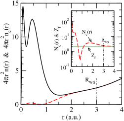
Figure 1: Main plot: The radial density $4\pi r^{2}n(r)$ in a.u. for metallic Al at $k_{\scriptscriptstyle B}T=5$ eV (solid black curve) integrates to $Z=13$ for $r\leq R_{\text{\tiny WS}}=2.991~{}a_{0}$. The continuum contribution $4\pi r^{2}n_{c}(r)$ (dashed red curve), also in a.u., integrates to 3 for $r\leq R_{\text{\tiny WS}}$. The bound $1s$, $2s$, and $2p$ shells are completely occupied at this temperature. Inset: The dashed red curve illustrates the Friedel oscillations of the continuum density and shows how $N_{c}(r)=n_{c}(r)V_{\text{\tiny WS}}$ converges to $Z_{f}=n_{e}V_{\text{\tiny WS}}$ (solid green line) for $r>R_{\text{\tiny WS}}$. The chemical potential predicted by the model is $\mu=0.2406$ a.u. and the number of free electrons per ion is $Z_{f}=2.146$.

The quantum-mechanical model here, which is discussed in Ref. JGB:06 , is a nonrelativistic version of the Inferno model of Liberman DL:79 and the more recent Purgatorio model of Wilson et al. BS:06 ; it is similar to the nonrelativistic average-atom model described by Blinski and Ishikawa BI:95 . Specifically, each electron in the ion is assumed to satisfy the central-field Schrödinger equation

$$\left[\frac{p^{2}}{2}-\frac{Z}{r}+V\right]\psi_{a}({\bm{r}})=\epsilon_{a}\,\psi_{a}({\bm{r}}),$$ (3)

where $a=(n,l)$ for bound states or $(\epsilon,l)$ for continuum states. Atomic units (a.u.) where $e=\hbar=m=4\pi\epsilon_{0}=1$ are used here. In particular, 1 a.u. in energy equals 2 Rydbergs (27.211 eV), and 1 a.u. in length equals 1 Bohr radius $a_{0}$ (0.529 Å).

The wave function $\psi_{a}({\bm{r}})$ is decomposed in a spherical basis as

$$\psi_{a}({\bm{r}})=\frac{1}{r}P_{a}(r)\,Y_{l_{a}m_{a}}(\hat{r})\,\chi_{\sigma_{a}},$$ (4)

where $Y_{lm}(\hat{r})$ is a spherical harmonic and $\chi_{\sigma}$ is a two-component electron spinor. The bound and continuum radial functions $P_{a}(r)$ are normalized as

$$\int_{0}^{\infty}\!\!dr\,P_{nl}(r)\,P_{n^{\prime}l}(r) ={}\delta_{nn^{\prime}},$$ (5)

$$\int_{0}^{\infty}\!\!dr\,P_{\epsilon l}(r)\,P_{\epsilon^{\prime}l}(r) ={}\delta(\epsilon-\epsilon^{\prime}),$$ (6)

respectively. The central potential $V(r)$ in Eq. (3) is taken to be the self-consistent Kohn-Sham potential kohnsham

$$V(r)=4\pi\!\int\!\frac{1}{r_{>}}\,r^{\prime 2}\,n(r^{\prime})\,dr^{\prime}-\bigg{[}\frac{3}{\pi}\,n(r)\bigg{]}^{\!\frac{1}{3}},$$ (7)

where the first term in the right-hand side is the direct screening potential with $r_{>}=\text{max}(r,\,r^{\prime})$ and the second term is the Kohn-Sham exchange potential. While electron-electron interactions inside the Wigner-Seitz cells are reasonably well accounted for by this simple model, it should be noted that eigenvalues in the Kohn-Sham potential are poor approximations to ionization energies, leading to inaccurate thresholds and peaks of bound-free contributions to $S(k,\omega)$, which can differ from experiment by 20 – 30%. The electron density $n(r)$ in Eq. (7) has contributions from bound states $n_{b}(r)$ and from continuum states $n_{c}(r)$,

$$n(r)=n_{b}(r)+n_{c}(r).$$ (8)

The bound-state contribution to the density $n_{b}(r)$ is

$$4\pi r^{2}n_{b}(r)=\sum_{nl}\frac{2(2l+1)}{1+\exp[(\epsilon_{nl}-\mu)/k_{\scriptscriptstyle B}T]}\,P_{nl}(r)^{2},$$ (9)

where $\epsilon_{nl}$ is the bound-state energy, $\mu$ is the chemical potential, and the sum over $(n,l)$ ranges over all bound subshells. The continuum contribution to the density $n_{c}(r)$ is given by

$$4\pi r^{2}n_{c}(r)=\sum_{l}\int_{0}^{\infty}\!\!d\epsilon\,\frac{2(2l+1)}{1+\exp[(\epsilon-\mu)/k_{\scriptscriptstyle B}T]}\,P_{\epsilon l}(r)^{2}.$$ (10)

Finally, the chemical potential $\mu$ is chosen to ensure charge neutrality inside the WS cell:

$$Z=\int_{r\leq R_{\text{\tiny WS}}}\!\!n(r)\,d^{3}r\equiv\int_{0}^{R_{\text{\tiny WS}}}\!\!4\pi r^{2}n(r)\,dr\ .$$ (11)

Equations (3–11) above are solved self-consistently to give the chemical potential $\mu$, the potential energy function $V(r)$ and the electron density $n(r)$.

The upper limit in Eq. (9) is determined by systematic trial and error. The values of $n$ and $l$ are increased starting from $n=1$ and $l=0$. If a state is bound, it is included in the sum, otherwise not. At metallic densities and temperatures below 100 eV (warm dense matter) fewer than a dozen states typically bind. To carry out the sum-integral in Eq. (10) for the continuum density, we typically use 12 partial waves ($l$) and 40 to 50 energy points ($\epsilon$) for each partial wave. The energy grid for the integral in Eq. (10) is chosen using a modified Gauss-Laguerre scheme. Thus, one is faced with solving a system of roughly 500 coupled second-order differential equations. These equations are solved iteratively using a predict-correct scheme based on Adam’s method (book, , Chap. 2.3).

The boundary conditions used in solving Eq. (3) deserve some mention. Bound-state wave functions and their derivatives are matched at the boundary $r=R_{\text{\tiny WS}}$ to solutions outside the WS sphere (where $V=0$) that vanish exponentially as $r\to\infty$. Similarly, continuum functions and their derivatives are matched to phase-shifted free-particle wave functions at $r=R_{\text{\tiny WS}}$. It should be noticed that the continuum density $n_{c}(r)$ inside the WS sphere, which oscillates as predicted by Freidel JF:54 , is distinctly different from the uniform free electron density $n_{e}$. In the present model, $n_{c}(r)$ smoothly approaches $n_{e}$ outside the sphere. These points are illustrated in Fig. 1, where the bound-state and continuum densities are plotted for Al at metallic density and temperature $k_{\scriptscriptstyle B}T=5$ eV. Occupation numbers of bound states and continuum partial-wave states inside the WS sphere are given along with bound-state eigenvalues in Table 1.

Table 1: Aluminum at density 2.70 g/cc and $k_{\scriptscriptstyle B}T=5$ eV. Bound-state and continuum partial-wave occupation numbers inside the WS sphere are given, along with bound-state eigenenergies. The Ne-like core is seen to be almost completely occupied. The sum of the bound-state and continuum occupation numbers is precisely $Z=13$.

Bound States				Continuum
State	occ#	$\epsilon$(eV)		$l$	occ#
$1s$	2.0000	-1485.07		0	0.9130
$2s$	2.0000	-92.16		1	1.3263
$2p$	5.9998	-54.87		2	0.6192
				3	0.1173
				4	0.0209
				5	0.0031
				6	0.0004
				7	0.0000
$N_{b}$	9.9998			$N_{c}$	3.0002

The boundary conditions used here differ from those used by Sahoo et al. in Ref. SG:08 , where the first derivative of the wave function is required to vanish at $R_{\text{\tiny WS}}$. The differences in boundary conditions lead to major differences in the average-atom structure. For example, the model used in Ref. SG:08 predicts that the $M$ shell of metallic Al is partially occupied at temperatures $k_{\scriptscriptstyle B}T\leq 10$ eV, whereas the present model predicts that the $M$ shell is empty in this temperature range. Consequences of such differences are discussed later in Sec. 4.

3 Dynamic Structure Function

As noted in the introduction, the theoretical model developed by Gregori et al. GG:03 , with input from the average-atom model, is used here to evaluate the dynamic structure function $S(k,\omega)$. The ion-ion contribution $S_{ii}(k,\omega)$ is evaluated in terms of Fourier-transforms of electron densities and the static ion-ion structure function $S_{ii}(k)$. Formulas for $S_{ii}(k)$ are given in Ref. AD:98 . Here, we use modified formulas that include options discussed in Ref. GGL:06 for different electron and ion temperatures. The dominant effect of different electron and ion temperatures is to modify the relative size of elastic to inelastic contributions to $S(k,\omega)$. The use of different temperatures is, therefore, a convenient tool for fitting experimental data, even in cases where equilibrium is reached. The inability to fit experimental data in some equilibrium cases without such an artifice is a weakness in the present scheme and is the subject of current research. The electron-electron contribution $S_{ee}(k,\omega)$ is expressed in terms of the dielectric function $\epsilon(k,\omega)$ of the free electrons which in turn is evaluated using the random-phase approximation (RPA). Plasmon resonances are present in $S_{ee}(k,\omega)$ at low momentum transfers $k$. Finally, bound-state contributions to the dynamic structure function are evaluated using average-atom bound-state wave functions for the initial state. The final-state continuum wave function is described in two different ways: (1) approximating the final-state by a plane wave as in Ref. SG:08 , and (2) using an average-atom final-state that approaches a plane wave asymptotically. There are dramatic differences between these two choices, especially at low momentum transfers. The more realistic average-atom choice automatically includes ionic Coulomb-field effects.

3.1 Ion-Ion Structure Function

The contribution to the dynamic structure function from elastic scattering by electrons following the ion motion $S_{ii}(k,\omega)$ is expressed in terms of the corresponding static ion-ion structure function $S_{ii}(k)$ as:

$$S_{ii}(k,\omega)=|f(k)+q(k)|^{2}\,S_{ii}(k)\,\delta(\omega).$$ (12)

In the above, $f(k)$ is the Fourier transform of the bound-state density and $q(k)$ is the Fourier transform of the density of electrons that screen the ionic charge. In the average-atom approximation, the screening electrons are the continuum electrons inside the Wigner-Seitz sphere and

$$f(k)+q(k)=4\pi\!\int_{0}^{R_{\scriptscriptstyle WS}}\!\!r^{2}\left[n_{b}(r)+n_{c}(r)\right]j_{0}(kr)\,dr,$$ (13)

where $j_{0}(z)$ is a spherical Bessel functions of order $0$. Note that $f(0)+q(0)=Z$ in the average-atom model. In the applications discussed later, $\delta(\omega)$ is replaced by an “instrumental” Gaussian, with full-width at half maximum = 10 eV. This value is chosen because typical experiments in Be DL:09 utilize a spectrometer with a 10-eV instrument width and use a Cl Ly-$\alpha$ source at 2.96 keV.

Approximate schemes to evaluate the static structure functions $S_{ii}(k)$ are discussed, for example, in Ref. JPH:06 . Here, we follow Gregori et al. GG:03 and make use of formulas given by Arkhipov and Davletov AD:98 that account for both quantum-mechanical and screening effects. The function $S_{ii}(k)$ in Ref. AD:98 is expressed in terms of the Fourier transform of the ion-ion interaction potential $\Phi_{ii}(r)$ through the relation:

$$S_{ii}(k)=1-\frac{n_{i}}{k_{\scriptscriptstyle B}T}\Phi_{ii}(k).$$ (14)

Different Electron and Ion Temperatures

In the average-atom model, $T$ is the electron temperature $T_{e}$ which, in equilibrium, is equal to the ion temperature $T_{i}$. To allow for different electron and ion temperatures, the equations for $S_{ii}(k)$ given by Arkhipov and Davletov AD:98 are modified following the prescription laid out by Gregori et al. GGL:06 . The electron temperature $T_{e}$ is replaced by an effective temperature $T_{e}^{\prime}$ that accounts for degeneracy effects at temperatures lower than the Fermi temperature $T_{F}$. Similarly, the ion temperature $T_{i}$ is replaced by an effective temperature $T_{i}^{\prime}$ that accounts for ion degeneracy effects at temperatures lower than the ion screened Debye temperature $T_{D}$. Explicit formulas for $S_{ii}(k)$ are found in Ref. GGL:06 . The dramatic effect of different electron and ion temperatures on the static structure functions $S_{ii}(k)$ for metallic Be at $T_{e}=20$ eV are illustrated in the left panel of Fig. 2. This figure is similar to the upper-left panel of Fig. 1 in Ref. GGL:06 , which was obtained under similar condition. In the right panel of Fig. 2, contributions to $S_{ii}(k,\omega)$ for Be at $T_{e}=20$ eV and $T_{i}=2$ eV are shown.

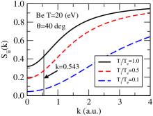
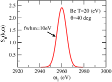
Figure 2: Left panel: $S_{ii}(k)$ is shown for Be metal at electron temperature $k_{\scriptscriptstyle B}T_{e}=20$ eV and ion-electron temperature ratios $T_{i}/T_{e}=(1,\ 0.5,\ 0.1)$ illustrated in solid, short-dashed and long dashed curves , respectively. The value $k$ = 0.543 corresponds to an incident photon $\omega_{0}=2960$ eV scattered at angle 40${}^{\circ}\!$. Right panel: $S_{ii}(k,\omega)$ in a.u. for Be metal at $k_{\scriptscriptstyle B}T_{e}=20$ eV and $T_{i}/T_{e}=0.1$, where the function $\delta(\omega)$ is replaced by a Gaussian of width 10 eV and $\omega_{1}=\omega_{0}-\omega$ is the energy of the scattered x-ray.

3.2 Electron-Electron Structure Function

The electron-electron structure function $S_{ee}(k,\omega)$ is expressed in terms of the free-electron dielectric function $\epsilon(k,\omega)$ through the relation Eq. (42) in Ref. CH:00 :

$$S_{ee}(k,\omega)=-\frac{1}{1-\exp(-\omega/k_{\scriptscriptstyle B}T)}\frac{k^{2}}{4\pi^{2}n_{e}}\text{Im}\left[\frac{1}{\epsilon(k,\omega)}\right].$$ (15)

We follow Gregori et al. GG:03 and evaluate the dielectric function in the random-phase approximation (RPA):

$$\epsilon(k,\omega)=1+\frac{4}{\pi k^{2}}\int_{0}^{\infty}\!\!{\mathcal{F}}(p)\,p^{2}dp\\ \times\int_{-1}^{1}d\mu\left[\frac{1}{k^{2}-2pk\mu+2\omega+i\nu}+\frac{1}{k^{2}+2pk\mu-2\omega-i\nu}\right],$$ (16)

where

$${\mathcal{F}}(p)=\frac{1}{1+\exp[(p^{2}/2-\mu)/k_{\scriptscriptstyle B}T]}$$ (17)

is the free-electron Fermi distribution. The parameter $\nu$ in Eq. 16 is a positive infinitesimal. The chemical potential $\mu$ is obtained from the average-atom model. It should be noted that the RPA dielectric function reduces to the Lindhard dielectric function Li:54 ; Ma:00 in the limit $k_{\scriptscriptstyle B}T\to 0$, where ${\mathcal{F}}(p)$ reduces to a unit step function that vanishes for $p>k_{\scriptscriptstyle F}$. In the finite $T$ case, we find

$$\int_{-1}^{1}\frac{d\mu}{k^{2}-2pk\mu+2\omega+i\nu} =\ \frac{1}{2pk}\,\ln\!\left[\frac{k^{2}+2pk+2\omega+i\nu}{k^{2}-2pk+2\omega+i\nu}\right]$$ (18)

$$\int_{-1}^{1}\frac{d\mu}{k^{2}+2pk\mu-2\omega-i\nu} =\ \frac{1}{2pk}\,\ln\!\left[\frac{k^{2}+2pk-2\omega-i\nu}{k^{2}-2pk-2\omega-i\nu}\right].$$ (19)

From the above expressions, it is clear that $\text{Re}[\epsilon(k,\omega)]$ is an even function of $\omega$ and that $\text{Im}[\epsilon(k,\omega)]$ is an odd function of $\omega$. Therefore, we can limit ourselves to cases where $\omega$ is positive. For $\omega>0$, one obtains in the limit $\nu\to 0+$,

$$\lim_{\nu\to 0}\left\{\ln\left[\frac{k^{2}+2pk+2\omega+i\nu}{k^{2}-2pk+2\omega+i\nu}\right]+\ln\left[\frac{k^{2}+2pk-2\omega-i\nu}{k^{2}-2pk-2\omega-i\nu}\right]\right\}\\ =\ln\left|\frac{k^{2}+2pk+2\omega}{k^{2}-2pk+2\omega}\right|+\ln\left|\frac{k^{2}+2pk-2\omega}{k^{2}-2pk-2\omega}\right|\\ +i\pi\ \text{only in the interval}\ |k^{2}-2\omega|\leq 2pk\leq k^{2}+2\omega.$$ (20)

It follows that

$$\text{Re}[\epsilon(k,\omega)]=1+\frac{2}{\pi k^{3}}\int_{0}^{\infty}{\mathcal{F}}(p)\,p\,dp\\ \times\left[\ln\left|\frac{k^{2}+2pk+2\omega}{k^{2}-2pk+2\omega}\right|+\ln\left|\frac{k^{2}+2pk-2\omega}{k^{2}-2pk-2\omega}\right|\right]$$ (21)

and

$$\text{Im}[\epsilon(k,\omega)]=\frac{2}{k^{3}}\int_{a}^{b}{\mathcal{F}}(p)\,p\,dp=\frac{2k_{\scriptscriptstyle B}T}{k^{3}}\log\left[\frac{1+\exp[(\mu-a^{2}/2)/k_{\scriptscriptstyle B}T]}{1+\exp[(\mu-b^{2}/2)/k_{\scriptscriptstyle B}T]}\right]$$ (22)

with $a=|2\omega-k^{2}|/2k$ and $b=(2\omega+k^{2})/2k$. From Eq. (15) and the fact that $\text{Im}[1/\epsilon(k,\omega)]$ is an odd function of $\omega$, it follows that

$$S_{ee}(k,\omega)=\exp(\omega/{k_{\scriptscriptstyle B}T})S_{ee}(k,-\omega).$$ (23)

Therefore, in the absence of bound-state contributions, measuring the cross-section ratio at down-shifted and up-shifted plasmon peaks, provides an experimental method for determining the plasma temperature.

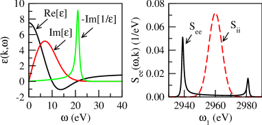
Figure 3: Left panel: Real and Imaginary parts of the dielectric function $\epsilon(k,\omega)$ are plotted along with $-\text{Im}[1/\epsilon]$ for coherent scattering of a 2960-eV photon at 20${}^{\circ}\!$ from Be metal at $k_{\scriptscriptstyle B}T=18$ eV. Right panel: The resulting electron-electron structure function $S_{ee}(k,\omega)$ (solid line) is shown together with $S_{ii}(k,\omega)$ (dashed line) which has an instrumental width of 10 eV. In this example $k=0.2757$ a.u. and $\omega_{1}=2960-\omega$ (eV) is the energy of the scattered x-ray.

The real and imaginary parts of $\epsilon(k,\omega)$, along with $-\text{Im}[1/\epsilon(k,\omega)]$, are shown in the left panel of Fig. 3 for Be metal at temperature $k_{\scriptscriptstyle B}T=18$ eV. A plasmon peak, associated with coherent scattering of the incident x-ray by the electrons in the plasma, is seen near $\omega=20$ eV, where the real part of the dielectric function vanishes. The corresponding structure function $S_{ee}(k,\omega)$, illustrating up- and down-shifted plasmon features, is shown in the right-hand panel. For comparison purposes, the elastic-scattering structure function $S_{ii}(k,\omega)$ is also shown in the right-hand panel. The functions displayed in this plot correspond to scattering of an incident 2960-eV photon at an angle 20${}^{\circ}\!$. The classical plasma frequency for this case ($n_{e}=2.05\times 10^{23}$ cc^-1) is $\omega_{\text{pl}}=16.8$ eV.

The amplitude and width of plasmon peaks is governed by the coherence parameter $\alpha=1/(\lambda_{s}k)$, defined in Eqs. (5-7) of Ref. GR:09 . Here, $\lambda_{s}$ is the shielding length given by

$$\lambda_{s}=\sqrt{\frac{k_{\scriptscriptstyle B}TF_{1/2}(\mu/{k_{\scriptscriptstyle B}T})}{4\pi n_{e}F_{-1/2}(\mu/{k_{\scriptscriptstyle B}T})}}\,,$$ (24)

where $F_{j}(x)$ is a complete Fermi-Dirac integral,

$$F_{\nu}(x)=\frac{1}{\Gamma(1+\nu)}\int_{0}^{\infty}\!\!dy\,\frac{y^{\nu}}{1+\exp(y-x)}\,.$$ (25)

For the example shown in Fig. 3, the screening length $\lambda_{s}=1.440$ and the corresponding coherence parameter $\alpha=2.520$, so one expects and observes plasmon resonances. At values of $\alpha$ less than than one, coherent scattering by the plasma no longer occurs and the plasmon peak in the dielectric function disappears. An example of this behavior is illustrated in Fig. 4, where the dielectric function for scattering of a 2960-eV photon at 90${}^{\circ}\!$ from Be metal at $k_{\scriptscriptstyle B}T=18$ eV is illustrated. The screening radius in this case remains unchanged $\lambda_{s}=1.440$, but the momentum transfer increases to $k=1.123$ and the resulting coherence parameter is $\alpha=0.6188$. Therefore, as expected, all signs of plasmon resonances are absent in $S_{ee}(k,\omega)$.

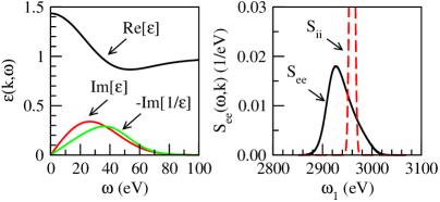
Figure 4: Left panel: Real and Imaginary parts of the dielectric function $\epsilon(k,\omega)$ are plotted along with $-\text{Im}[1/\epsilon]$ for incoherent scattering of a 2960-eV photon at 90${}^{\circ}\!$ from Be metal at $k_{\scriptscriptstyle B}T=18$ eV. Right panel: The electron-electron structure function $S_{ee}(k,\omega)$ (solid line) is shown together with $S_{ii}(k,\omega)$ (dashed line) which is assumed to have an instrumental width of 10 eV. The corresponding momentum transfer is $k=1.123$ a.u. and $\omega_{1}=2960-\omega$ (eV) is the energy of the scattered x-ray.

3.3 Bound-Free Structure Function

The contribution to the dynamic structure function for Thomson scattering from ionic bound states $S_{b}(k,\omega)$ is the sum over contributions from individual subshells with quantum numbers $(n,l)$:

$$S_{b}(k,\omega) =\ \sum_{nl}S_{nl}(k,\omega)$$ (26)

$$S_{nl}(k,\omega) =\ \frac{o_{nl}}{2l+1}\sum_{m}\int\frac{p\,d\Omega_{p}}{(2\pi)^{3}}\,\left|\int\!\!d^{3}r\,\psi^{\dagger}_{\bm{p}}(\bm{r})\,e^{i\bm{k}\cdot\bm{r}}\,\psi_{nlm}(\bm{r})\right|^{2}_{\epsilon_{p}=\omega+\epsilon_{nl}},$$ (27)

where $o_{nm}$ is the fractional occupation number of subshell $(n,l)$, and ${\bm{k}}={\bm{k}}_{0}-{\bm{k}}_{1}$ and $\omega=\omega_{0}-\omega_{1}$ are the momentum and energy transfers, respectively, from the incident to the scattered photon as defined in Eq. (1). In the above, $\psi_{\bm{p}}(\bm{r})$ is an average-atom wave function that approaches a plane wave $e^{i\bm{p\cdot r}}$ asymptotically. We consider two cases below: firstly, the case where $\psi_{\bm{p}}(\bm{r})$ is approximated by a plane wave and secondly, the case where $\psi_{\bm{p}}(\bm{r})$ is an average-atom scattering function that approaches a plane wave asymptotically.

Plane-wave final states

Approximating the final state wave function by a plane wave $\psi_{\bm{p}}(\bm{r})=e^{i\bm{p}\cdot\bm{r}}$, the bound-free structure function in Eq. (27) can be rewritten as

$$S_{nl}(k,\omega)=\frac{o_{nl}}{2l+1}\sum_{m}\int\frac{p\,d\Omega_{p}}{(2\pi)^{3}}\left|\int\!d^{3}r\,e^{i\bm{q}\cdot\bm{r}}\,\psi_{nlm}(\bm{r})\right|^{2},$$ (28)

where $\epsilon_{p}=\omega+\epsilon_{nl}$ and ${\bm{q}}={\bm{k}}-{\bm{p}}$. Note that ${\bm{q}}$ is the momentum transferred to the ion. This expression may be simplified to

$$S_{nl}(k,\omega)=\frac{o_{nl}}{\pi k}\int_{|p-k|}^{p+k}q\,dq\,|K_{nl}(q)|^{2},$$ (29)

$$K_{nl}(q)=\int_{0}^{\infty}\!\!r\,dr\,j_{l}(qr)P_{nl}(r).$$ (30)

$S_{nl}(k,\omega)$ in Eq. (29) depends implicitly on $\omega$ through the relation

$$p=\sqrt{2(\omega+\epsilon_{nl}})\ .$$

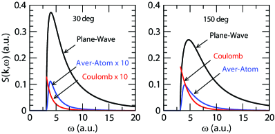
Figure 5: The beryllium $K$-shell structure function $S_{1s}(k,\omega)$ is shown for incident photon energy 2960 eV and scattering angles 30${}^{\circ}\!$ and 150${}^{\circ}\!$. The black curves show plane-wave results, the blue lines show the result obtained using an average-atom final-state wave function and the red lines show exact nonrelativistic Coulomb results. The dramatic suppression of average-atom and Coulomb structure functions at forward angles (the corresponding curves are multiplied by 10) is evident in the left panel.

Average-atom final states

In the average-atom approach, the final state wave function consists of a plane wave plus an incoming spherical wave. (N.B. An outgoing spherical wave is associated with an incident electron. Time-reversal invariance, therefore, requires that a converging spherical wave be associated with an emerging electron.) The scattering wave function $\psi_{\bm{p}}(\bm{r})$ in Eq. (27) may be written

$$\psi_{\bm{p}}(\bm{r})=\frac{4\pi}{p}\sum_{l_{1}m_{1}}i^{\,l_{1}}e^{-i\delta_{l_{1}}}\frac{1}{r}P_{\epsilon l_{1}}(r)\,Y^{\ast}_{l_{1}m_{1}}(\hat{p})\,Y_{l_{1}m_{1}}(\hat{r}),$$ (31)

where the continuum wave function is normalized to a phase-shifted sine wave asymptotically

$$P_{\epsilon l}(r)\to\sin(pr-l\pi/2+\delta_{l}).$$ (32)

The factor $e^{i\bm{k\cdot r}}$ in Eq. (27) is expanded as

$$e^{1\bm{k\cdot r}}=4\pi\sum_{l_{2}m_{2}}i^{\,l_{2}}j_{l_{2}}(kr)\,Y^{\ast}_{l_{2}m_{2}}(\hat{k})\,Y_{l_{2}m_{2}}(\hat{r}).$$ (33)

The bound-free structure function in Eq. (27) may then be expressed as

$$S_{nl}=\frac{o_{nl}}{2l+1}\int\frac{p\,d\Omega_{p}}{(2\pi)^{3}}\sum_{m}\left|J_{nlm}\right|^{2},$$ (34)

where

$$J_{nlm}=\frac{(4\pi)^{2}}{p}\sum_{l_{1}l_{2}}i^{\,l_{2}-l_{1}}\,I_{l_{1}l\,l_{2}}(p,k)\!\sum_{m_{1}m_{2}}\!\left<l_{1}m_{1}|Y_{lm}|l_{2}m_{2}\right>Y_{l_{1}m_{1}}(\hat{p})\,Y_{l_{2}m_{2}}^{\ast}(\hat{k}),$$ (35)

with

$$I_{l_{1}l\,l_{2}}(p,k)=\frac{1}{p}\,e^{i\delta_{l_{1}}\!\!(p)}\!\int_{0}^{\infty}\!drP_{\epsilon l_{1}}(r)P_{nl}(r)j_{l_{2}}(kr)$$ (36)

and

$$\left<l_{1}m_{1}|Y_{lm}|l_{2}m_{2}\right>=\int\!d\Omega\,Y^{\ast}_{l_{1}m_{1}}(\hat{r})\,Y_{lm}(\hat{r})\,Y_{l_{2}m_{2}}(\hat{r}).$$ (37)

Squaring $J_{nlm}$, integrating over angles of $\bm{p}$, and summing over magnetic quantum numbers, one obtains

$$S_{nl}=\frac{2p}{\pi}o_{nl}\sum_{l_{1}l_{2}}A_{l_{1}l\,l_{2}}\left|I_{l_{1}l\,l_{2}}(p,k)\right|^{2}$$ (38)

where

$$A_{l_{1}l\,l_{2}}=(2l_{1}+1)(2l_{2}+1)\left(\begin{array}[]{ccc}l_{1}&l&l_{2}\\ 0&0&0\end{array}\right)^{\!2}.$$ (39)

In Fig. 5, several calculations of the structure function $S_{1s}(k,\omega)$ are compared for a photon of incident energy 2960 eV scattered at 30${}^{\circ}\!$ ($k=0.411$ a.u.) and 150${}^{\circ}\!$ ($k=1.533$ a.u.) from the $K$ shell of beryllium metal at $k_{\scriptscriptstyle B}T$ = 20 eV. The results of calculations carried out using average-atom final states are smaller than those using plane-wave final states by a factor of about 40 at $\theta=30^{\circ}\!$ and 2.5 at $\theta=150^{\circ}\!$. This suppression is a characteristic Coulomb field effect. Indeed, exact nonrelativistic Coulomb-field calculations of Thomson scattering EP:70 , with nuclear charge adjusted to align the Coulomb and average-atom thresholds, illustrated by the curves labeled “Coulomb” in Fig. 5, show a similar suppression.

The situation is quite different at much higher momentum transfer. This fact is illustrated in the left panel of Fig. 6, where we consider scattering of an 18-keV photon at 130${}^{\circ}\!$ ($k=8.750$ a.u.) from Be metal at $k_{\scriptscriptstyle B}T$ = 12 eV. The solid black curve shows the bound-state contribution to the $S(k,\omega)$ evaluated using an average-atom final state, while the dashed green line shows the contribution evaluated using a plane-wave final state. In this high-momentum transfer case, the two calculations differ qualitatively near threshold and the peak energies differ by a few percent, but the average-atom and plane-wave results are otherwise quite similar.

In the right panel of Fig. 6, we consider a more complex example, scattering of a 9300-eV x-ray at 130${}^{\circ}\!$ ($k=4.521$ a.u.) from tin metal at $k_{\scriptscriptstyle B}T=10$ eV. Contributions from individual subshells are shown together with their sum $S_{b}(k,\omega)$.

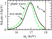
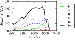
Figure 6: Left panel: The dynamic structure function for the $1s$ state of Be metal at $k_{\scriptscriptstyle B}T=12$ eV is shown for scattering of an incident x-ray with energy $\omega_{0}$ = 18-keV x-ray at 130${}^{\circ}\!$. The solid black and dashed green lines are results calculated using average-atom and plane-wave final states, respectively. The dashed red line is the elastic scattering contribution $S_{ii}(k,\omega)$ with instrumental width 10 eV. Right panel: The total bound-free dynamic structure function $S_{b}(k,\omega)$ with average-atom final states is shown for tin ($Z=50$) at metallic density and $k_{\scriptscriptstyle B}T=10$ eV is shown, along with contributions from individual subshells. The incident x-ray energy is $\omega_{0}=9.3$ keV and the scattering angle is 130${}^{\circ}\!$. In the above, $\omega_{1}=\omega_{0}-\omega$ is the energy of the scattered x-ray.

4 Applications

The scheme developed in the previous sections is applied to several examples of current or possible future interest. The example of hydrogen at electron density 10²⁴ cc^-1 and temperature 50 eV is considered first. In this example, the H ion is completely stripped and inelastic scattering is determined completely by $S_{ee}(k,\omega)$. The plasmon resonances present in the hydrogen spectrum at forward scattering angles fade rapidly with increasing angle. The case of beryllium metal at 18 eV, which has been well studied both theoretically and experimentally, is considered next and good agreement is found between average-atom predictions and experimental data. For beryllium, the bound-state contribution is small and beyond the range of available experimental data. As a third example, calculations of $S(k,\omega)$ for scattering of 9.3-keV and 3.1-keV x-rays from aluminum metal at $k_{\scriptscriptstyle B}T=5$ eV are evaluated and compared with the average-atom predictions by Sahoo et al. SG:08 . Finally, Thomson scattering of 9.3-keV x-rays from titanium and tin at 30${}^{\circ}\!$ and 130${}^{\circ}\!$ are considered to illustrate cases where bound-state contributions are the dominant features of the scattered x-ray spectrum. In Table 2, we list some important average-atom properties for the elements considered in the following subsections.

Table 2: Average-atom parameters for the examples of hydrogen, beryllium, aluminum, titanium, and tin presented in Sec. 4.

	H	Be	Al	Ti	Sn
$k_{\scriptscriptstyle B}T$ (eV)	50	18	5	10	10
$\rho$ (g/cc)	1.931	1.635	2.700	4.540	7.310
$R_{\scriptscriptstyle WS}$ $(a_{0})$	1.118	2.452	2.991	3.044	3.515
$\mu$ (a.u.)	1.091	-0.531	0.241	-0.044	-0.071
$N_{\text{bound}}$	0	1.966	10.000	17.341	45.622
$N_{\text{cont}}$	1	2.036	3.000	4.659	4.378
$Z_{f}$	0.867	1.647	2.146	2.322	3.374
$n_{e}$ ($10^{23}$ cc-1)	10	1.800	1.292	1.326	1.251

4.1 Hydrogen

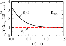
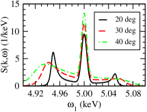
Figure 7: Left panel: The continuum density $n_{c}(r)$ inside the WS sphere for hydrogen at $k_{\scriptscriptstyle B}T=50$ eV and density 1.931 g/cc is seen to converge smoothly to the free-electron density $n_{e}=10^{24}$ cc^-1 beyond the WS radius $R_{\scriptscriptstyle WS}$. Right panel: The dynamic structure function $S(k,\omega)$ for H at $k_{\scriptscriptstyle B}T=50$ eV and $n_{e}=10^{24}$ cc^-1 is plotted for scattering of a 5-keV photon at angles 20${}^{\circ}\!$, 30${}^{\circ}\!$ and 40${}^{\circ}\!$, and $\omega_{1}=5-\omega$ (keV) is the energy of the scattered x-ray.

In the average-atom model, a density $\rho=1.931$ g/cc is required at $k_{\scriptscriptstyle B}T=50$ eV to achieve free-electron density $n_{e}=10^{24}$ cc^-1. Physical properties of the plasma under these conditions are listed in the second column of Table 2. The single electron in hydrogen is completely stripped, leaving only the continuum inside the WS sphere. The continuum density $n_{c}(r)$ merges into the uniform free-electron density $n_{e}$ outside the sphere. The total number of electrons inside the WS sphere $N_{c}=4\pi\int_{0}^{R_{\text{\tiny WS}}}r^{2}n_{c}(r)dr=1$, however, the number of free electrons per ion is $Z_{f}=0.867$. These points are illustrated in the left panel of Fig, 7.

Since there are no bound electrons, only $S_{ee}(k,\omega)$ contributes to the inelastic scattering. The dynamic structure functions for scattering of a 5-keV x-ray at angles 20${}^{\circ}\!$, 30${}^{\circ}\!$ and 40${}^{\circ}\!$ are shown in the right panel of Fig. 7. The prominent plasmon peaks at $\theta=20^{\circ}\!$ wash out at as the scattering angle (and momentum transfer $k$) is increased. For this particular case, the screening length $\lambda_{s}=1.071$ a.u. differs only slightly from the WS radius $R_{\text{\tiny WS}}=1.118$ a.u.. The values of the coherence parameter $\alpha$ for $\theta=(20^{\circ}\!,\ 30^{\circ}\!,\ 40^{\circ}\!)$ are $\alpha=(2.005,\ 1.345,\ 1.018)$, respectively. The resonant features in Fig. 7 are seen to be distinct for $\alpha>1$ but disappear as $\alpha$ approaches 1. It should be noted that the (unperturbed) plasma frequency for hydrogen at $n_{e}=10^{24}$ cc^-1 is $\omega_{\text{pl}}=37.1$ eV.

4.2 Beryllium

In the left panel of Fig. 8, the dynamic structure function for scattering of a 2963-eV photon at 40${}^{\circ}\!$ from beryllium (density = 1.635 g/cc) at $k_{\scriptscriptstyle B}T=18$ eV is shown. The $L$-shell electrons are completely stripped under these conditions but the $K$ shell remains 97% occupied. The ion temperature, which governs the amplitude of the elastic peak, is chosen to be $2.1$ eV in this example. For the case at hand, the coherence parameter is $\alpha=1.21>1$, so one expects and observes plasmon peaks in the scattering intensity profile. In the average-atom approximation, the threshold energy for bound-state contributions is the average-atom eigenvalue $\epsilon_{1s}=-86.8$ eV. (As mentioned earlier, average-atom eigenvalues are inaccurate approximations to removal energies. The average-atom threshold $|\epsilon_{1s}|$ is 20% smaller than the measured $K$-shell threshold 111 eV in beryllium metal PRD .) In the average-atom approximation, bound-state contributions to $S(k,\omega)$ from $K$-shell electrons have a threshold at $\omega_{1}=2963-86.8=2876.2$ eV. The $K$-shell contribution multiplied by 50 is shown in the left panel. The average-atom parameters used in this calculation are listed in column three of Table 2.

To validate the present average-atom model against experimental data, a Be experiment done at the Omega laser facility that used a Cl Ly-$\alpha$ source to scatter from nearly solid Be at an angle of 40^∘ is used. An electron temperature of 18 eV, ion temperature of 2.1 eV, and density of 1.635 g/cc used in the average-atom model gives an electron density of $1.8\times 10^{23}$ cc^-1, in agreement with the analysis in Ref. GD:12 . The right panel of Fig. 8 shows the experimental source function from the Cl Ly-$\alpha$ line as a blue dashed line. Because of satellite structure in the source we approximate the source by three lines: a Cl Ly-$\alpha$ line at 2963 eV with amplitude 1 and two satellites at 2934 and 2946 eV with relative amplitudes of 0.075 and 0.037, respectively. Doing the Thomson scattering calculation using the three weighted lines, we calculate the scattering amplitude for Thomson scattering (red solid line) and compare against the experimental data (black solid line) here. We observe excellent agreement within the experimental noise. Contributions from the bound $1s$ electrons, which have a threshold at 2876 eV, are beyond the range of the data shown in the right panel.

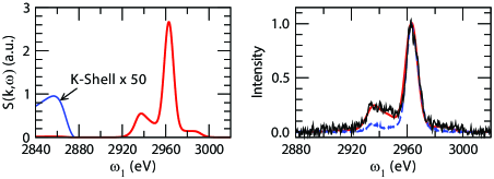
Figure 8: Left panel: Structure function $S(k,\omega)$ for scattering of a 2963-eV photon at 40^∘ from beryllium at $n_{e}=1.8\times 10^{23}$ cc^-1 and electron temperature $18$ eV. The bound-state contribution is scaled up by a factor of 50. Right panel: Intensities (arbitrary units) for scattering of a Cl Ly-$\alpha$ x-ray from beryllium at 40${}^{\circ}\!$ GD:12 ; measured data (black solid line), source function (blue dashed line), and the average-atom fit (red solid line). In the above, $\omega_{1}$ is the energy of the scattered x-ray.

4.3 Aluminum

As mentioned in the introduction, the present average-atom calculations disagree in various ways with those in Ref. SG:08 , where Thomson scattering from aluminum metal at several temperatures was considered. To clarify the differences, we compare results of the present calculations for the case of aluminum at $k_{\scriptscriptstyle B}T=5$ eV with the corresponding results presented in Ref. SG:08 . The dimensionless product $S(k,\omega)\,\omega_{\text{pl}}$ is shown for scattering of 9300-eV and 3100-eV x-rays in the left and right panels of Fig. 9, respectively. The upper and lower panels of Fig. 9 show results for scattering angles of 30${}^{\circ}\!$ and 130${}^{\circ}\!$, respectively. The plots in Fig. 9 can be compared directly with those in Fig. 6 and Fig. 7 of SG:08 , where similar plots for 9300-eV and 3100-eV x-ray energies can be found. The size and shape of the free-electron contributions shown in Fig. 9 are in agreement with those shown in the corresponding figures in SG:08 , however, the $L$-shell contributions to $S(k,\omega)$ in SG:08 are larger by a factor of approximately 5 than those shown in Fig. 9. Moreover, contributions from the $M$ shell, which dominate the spectrum just below the elastic peak in SG:08 are completely absent in Fig. 9. Owing to the differences in bound-free contributions $S_{b}(k,\omega)$, the present prediction for the aluminum dynamic structure function $S(k,\omega)$ differs in both size and shape from that given in SG:08 .

Differences in boundary conditions between the two average-atom models account for the presence or absence of bound $M$-shell electrons as discussed in Sec. 2. Furthermore, difference in the relative size of the $L$-shell contributions at forward angles may owe in part to the use of plane-wave final states in SG:08 . However, the substantial difference in size of the $L$-shell contributions at backward angles remains a mystery. The average-atom parameters for aluminum used in the present calculation are given in the fourth column of Table 2.

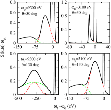
Figure 9: $S(k,\omega)\,\omega_{\text{pl}}$ is shown for scattering of 9300-eV and 3100-eV x-rays at 30${}^{\circ}\!$ and 130${}^{\circ}\!$ from Al metal at $k_{\scriptscriptstyle B}T$ = 5 eV. The short-dashed red curves are contributions $S_{ee}(k,\omega)$ from free electrons, the long-dashed green curves give contributions $S_{b}(k,\omega)$ from bound $2s$ and $2p$ electrons and the solid black curves show the total dynamic structure function. Instrumental widths of 0.1%$\omega_{0}$ were used. For Al metal at $k_{\scriptscriptstyle B}T$ = 5 eV, the plasma frequency is $\omega_{\text{pl}}=13.35$ eV. In the above figure, $\omega_{1}$ and $\omega_{0}$ are energies of the scattered and incident x-rays, respectively, and $\omega=\omega_{0}-\omega_{1}$.

4.4 Titanium & Tin

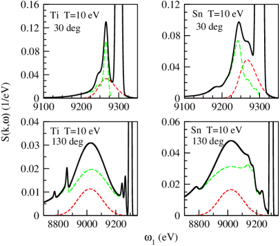
Figure 10: Left panels: $S(k,\omega)$ for scattering of a 9.3-keV x-ray at $\theta=30^{\circ}\!$ and 130${}^{\circ}\!$ from Ti metal at $k_{\scriptscriptstyle B}=10$ eV is shown in the solid black line. The free-electron contribution $S_{ee}(k,\omega)$ is shown in the short-dashed red line while the contribution from bound states $S_{b}(k,\omega)$ is shown in the long-dashed green line. Right panel: Same as left panel, except scattering from Sn metal at $k_{\scriptscriptstyle B}=10$ eV. Contributions from individual subshells of Sn are shown in the right panel of Fig. 10. In the figure above, $\omega_{1}=9300-\omega$ (eV) is the energy of the scattered x-ray.

Table 3: Comparison of the theoretical average-atom thresholds ($-\epsilon_{nl}$) and experimental thresholds from the NIST database PRD for contributions to $S_{b}(k,\omega)$ from individual subshells in titanium and tin.

Titanium					Tin
$nl$	theory	expt.	$\Delta$%		$nl$	theory	expt.	$\Delta$%
$2s$	512.7	563.7	9		$3d$	477.8	488.2	2
$2p$	426.8	457.5	7		$4s$	118.9	136.5	13
$3s$	45.4	60.3	25		$4p$	83.1	86.6	4
$3p$	22.8	34.6	34		$4d$	22.4	23.9	6
					$5s$	2.1	–	–

The average-atom model predicts that a titanium metal at 10 eV is in an Ar-like configuration with completely filled $K$ and $L$ shells together with 1.97 $3s$ electrons 5.36 $3p$ electrons in the $M$ shell. This is an interesting case where contributions to $S_{b}(k,\omega)$ from the $L$ and $M$ shells are substantial. In the left panels of Fig. 10, the dynamic structure function $S(k,\omega)$ is shown in the solid black line for an incident 9.3-keV x-ray scattered at 30${}^{\circ}\!$ and 130${}^{\circ}\!$. Contributions from $S_{b}(k,\omega)$ shown in the long-dashed green lines dominate the free-electron contributions $S_{ee}(k,\omega)$ shown in the short-dashed red lines. As seen in the lower-left panel, sharp features associated with excitation of the $M$ subshells ($3p$ and $3s$) show up just below the elastic peak at $\omega_{1}=\omega_{0}$, whereas features associated with excitation of the $L$ subshells ($2p$ and $2s$) show up 400 to 500 eV below the elastic peak. The bound-state thresholds for titanium are compared with measured thresholds from the National Institute for Standards & Technology (NIST) database PRD in Table 3.

Metallic tin at 10 eV has a Pd configuration with 45.6 bound electrons. The resulting dynamic structure function $S(k,\omega)$ is shown in the right panels of Fig. 10 for scattering angles of 30${}^{\circ}\!$ and 130${}^{\circ}\!$. The situation is similar to that for titanium; bound-free contributions dominate those from free-electrons. The irregularities in the bound-state contributions are associated with the onset of contributions from individual subshells. For scattering at 130${}^{\circ}\!$, contributions from individual subshells are shown in the right panel of Fig. 6. Average-atom thresholds for tin are compared with values from the NIST database PRD in Table 3.

5 Summary

A scheme for analysis of Thomson scattering from plasmas based on the average-atom model is presented. Given the plasma composition $(Z,A)$, density $\rho$ and temperature $T$, the model gives, in addition to the equation of state of the plasma, all parameters needed for a complete description of the Thomson scattering process. In particular, the average-atom code predicts wave functions for bound and continuum electrons, densities of bound, screening, and free electrons, and the chemical potential. Predictions of the present average-atom model disagree with those in Ref. SG:08 where a similar model with different boundary conditions was used. In the average-atom model used in Ref. SG:08 , $3d$ ($M$ shell) electrons are bound in metallic Al for temperatures between 2 and 10 eV, leading to substantial bound-state contributions to the dynamic structure function. In the present model, by contrast, the $M$ shell of metallic aluminum is vacant in the temperature range $k_{\scriptscriptstyle B}T\leq 10$ eV and the corresponding bound-state features are absent.

Elastic scattering from bound and screening electrons is treated here following the model proposed by Gergori et al. GG:03 which makes use of formulas for the static ion-ion structure function $S_{ii}(k)$ given by Arkhipov and Davletov AD:98 . Modifications suggested in Ref. GGL:06 to account for different electron and ion temperatures are also included. Specifically, in the applications considered here, the amplitude of the elastic peak is adjusted artificially by choosing an ion temperature that is different from the electron temperature, even in cases where equilibrium is expected. Such an adjustment was used to fit the experimental data for beryllium shown in Fig. 8. The dynamic structure function for scattering from free electrons depends sensitively on the free-electron dielectric function $\epsilon(k,\omega)$. Again, we follow the model proposed in Ref. GG:03 and evaluate the dielectric function in the random-phase approximation. The RPA dielectric function includes features such as plasmon resonant peaks that show up in experimental intensity profiles and can be used in connection with the principle of detailed balance to determine electron temperatures. Bound-state features are easily included in the present scheme, inasmuch as the average-atom model provides bound-state and continuum wave functions. Ionic Coulomb-field effects are features of calculations carried out using average-atom wave functions rather than plane waves to describe the final state electrons. In conclusion, the average-atom model provides a simple and consistent point of departure for the theoretical analysis of Thomson scattering from plasmas.

References

- (1) G. Gregori, S. Glenzer, R. Lee, D. Hicks, J. Pasley, G. Collins, P. Celliers, M. Bastea, J. Eggert, S. Pollaine, O. Landen, in Spectral Line Shapes, AIP Conference Proceedings, vol. 645, ed. by C. Back (2002), AIP Conference Proceedings, vol. 645, pp. 359–368
- (2) R. Lee, H. Baldis, R. Cauble, O. Landen, J. Wark, A. Ng, S. Rose, C. Lewis, D. Riley, J. Gauthier, P. Audebert, Laser Part. Beams 20, 527 (2002)
- (3) G. Gregori, S.H. Glenzer, W. Rozmus, R.W. Lee, O.L. Landen, Phys. Rev. E 67, 026412 (2003)
- (4) R. Lee, S. Moon, H. Chung, W. Rozmus, H. Baldis, G. Gregori, R. Cauble, O. Landen, J. Wark, A. Ng, S. Rose, C. Lewis, D. Riley, J. Gauthier, P. Audebert, J. Opt. Soc. Am. B 20, 770 (2003)
- (5) S.H. Glenzer, G. Gregori, R.W. Lee, F.J. Rogers, S.W. Pollaine, O.L. Landen, Phys. Rev. Lett. 90, 175002 (2003)
- (6) G. Gregori, S. Glenzer, O. Landen, J. Phys. A 36, 5971 (2003)
- (7) A. Höll, R. Redmer, G. Röpke, H. Reinholz, Eur. Phys. J. D 29, 159 (2004)
- (8) G. Gregori, S.H. Glenzer, O.L. Landen, Phys. Rev. E 74, 026402 (2006)
- (9) S.H. Glenzer, O.L. Landen, P. Neumayer, R.W. Lee, K. Widmann, S.W. Pollaine, R.J. Wallace, G. Gregori, A. Höll, T. Bornath, R. Thiele, V. Schwarz, W.D. Kraeft, R. Redmer, Phys. Rev. Lett. 98, 065002 (2007)
- (10) R. Thiele, T. Bornath, C. Fortmann, A. Höll, R. Redmer, H. Reinholz, G. Röpke, A. Wierling, S.H. Glenzer, G. Gregori, Phys. Rev. E 78, 026411 (2008)
- (11) A.L. Kritcher, P. Neumayer, H.J. Lee, T. Döppner, R.W. Falcone, S.H. Glenzer, E.C. Morse, Rev. Sci. Instrum. 79, 10E739 (2008)
- (12) R.R. Fäustlin, S. Toleikis, T. Bomath, L. Cao, T. Döppner, S. Düsterer, E. Förster, C. Fortmann, S.H. Glenzer, S. Göde, G. Gregori, A. Höll, R. Irsig, T. Laarmann, H.J. Lee, K.H. Meiwes-Broer, A. Przystawik, P. Radcliffe, R. Redmer, H. Reinholz, G. Röpke, R. Thiele, J. Tiggesbaeumker, N.X. Truong, I. Uschmann, U. Zastrau, T. Tschentscher, in Ultrafast Phenomena XVI, Springer Series in Chemical Physics, vol. 92, ed. by P. Corkum, S. DeSilvestri, K. Nelson, E. Riedle (2009), Springer Series in Chemical Physics, vol. 92, pp. 241–243. 16th International Conference on Ultrafast Phenomena, European Phys Soc, Stresa, Italy, Jun. 09-13, 2008
- (13) T. Döppner, O.L. Landen, H.J. Lee, P. Neumayer, S.P. Regan, S.H. Glenzer, High Energy Density Phys. 5, 182 (2009)
- (14) N.L. Kugland, G. Gregori, S. Bandyopadhyay, C.M. Brenner, C.R.D. Brown, C. Constantin, S.H. Glenzer, F.Y. Khattak, A.L. Kritcher, C. Niemann, A. Otten, J. Pasley, A. Pelka, M. Roth, C. Spindloe, D. Riley, Phys. Rev. E 80, 066406 (2009)
- (15) S.H. Glenzer, H.J. Lee, P. Davis, T. Döppner, R.W. Falcone, C. Fortmann, B.A. Hammel, A.L. Kritcher, O.L. Landen, R.W. Lee, D.H. Munro, R. Redmer, S. Weber, High Energy Density Phys. 6, 1 (2010)
- (16) M.S. Murillo, Phys. Rev. E 81, 036403 (2010)
- (17) S. Toleikis, T. Bornath, T. Döppner, S. Düsterer, R.R. Fäustlin, E. Förster, C. Fortmann, S.H. Glenzer, S. Göde, G. Gregori, R. Irsig, T. Laarmann, H.J. Lee, B. Li, K.H. Meiwes-Broer, J. Mithen, B. Nagler, A. Przystawik, P. Radcliffe, H. Redlin, R. Redmer, H. Reinholz, G. Röpke, F. Tavella, R. Thiele, J. Tiggesbaeumker, I. Uschmann, S.M. Vinko, T. Whitcher, U. Zastrau, B. Ziaja, T. Tschentscher, J. Phys. B 43, 194017 (2010)
- (18) R. Redmer, G. Röpke, Contrib. Plasm, Phys. 50, 970 (2010)
- (19) A.L. Kritcher, T. Döppner, C. Fortmann, O.L. Landen, R. Wallace, S.H. Glenzer, High Energy Density Phys. 7, 271 (2011)
- (20) A.J. Visco, R.P. Drake, S.H. Glenzer, T. Döppner, G. Gregori, D.H. Froula, M.J. Grosskopf, Phys. Rev. Lett. 108, 145001 (2012)
- (21) C. Fortmann, H.J. Lee, T. Döppner, R.W. Falcone, A.L. Kritcher, O.L. Landen, C. Niemann, S.H. Glenzer, Contrib. Plasma Phys. 52, 186 (2012)
- (22) U. Zastrau, T. Burian, J. Chalupsky, T. Döppner, T.W.J. Dzelzainis, R.R. Fäustlin, C. Fortmann, E. Galtier, S.H. Glenzer, G. Gregori, L. Juha, H.J. Lee, R.W. Lee, C.L.S. Lewis, N. Medvedev, B. Nagler, A.J. Nelson, D. Riley, F.B. Rosmej, S. Toleikis, T. Tschentscher, I. Uschmann, S.M. Vinko, J.S. Wark, T. Whitcher, E. Förster, Laser Part. Beams 30, 45 (2012)
- (23) S.H. Glenzer, R. Redmer, Rev. Mod. Phys. 81, 1625 (2009)
- (24) W.R. Johnson, C. Guet, G.F. Bertsch, J. Quant. Spectros. & Radiat. Transfer 99, 327 (2006)
- (25) S. Sahoo, G.F. Gribakin, G. Shabbir Naz, J. Kohanoff, D. Riley, Phys. Rev. E 77, 046402 (2008)
- (26) J. Chihara, J. Phys. F: Met. Phys. 17, 295 (1987)
- (27) J. Chihara, J. Phys.: Condens. Matter 12, 231 (2000)
- (28) R.P. Feynman, N. Metropolis, E. Teller, Phys. Rev. 75, 1561 (1949)
- (29) D.A. Liberman, Phys. Rev. B 20, 4981 (1979)
- (30) B. Wilson, V. Sonnad, P. Sterne, W. Isaacs, J. Quant. Spectros. Radiat. Transfer 99, 658 (2006)
- (31) T. Blenski, K. Ishikawa, Phys. Rev. E 51, 4869 (1995)
- (32) W. Kohn, L.J. Sham, Phys. Rev. 140, A1133 (1965)
- (33) W.R. Johnaon, Atomic Structure Theory (Springer-Verlag, 2007)
- (34) J. Friedel, Adv. Phys. 3, 507 (1954)
- (35) Y. Arkhipov, A. Davletov, Phys. Letts. A 227, 339 (1998)
- (36) J.P. Hansen, I.R. McDonald, Theory of Simple Liquids, 3rd edn. (Academic, London, Orlando, 2006)
- (37) J. Lindhard, Kgl. Danske Videnskab. Selskab, Mat.-Fys. Medd. 28, No. 8 (1954)
- (38) G.D. Mahan, Many-Particle Physics, 3rd edn. (Springer-Verlag, 2000)
- (39) P. Eisenberger, P.M. Platzman, Phys. Rev. A 2, 415 (1970)
- (40) physics.nist.gov/PhysRefData/FFast/html/form.html
- (41) S.H. Glenzer, T. Döppner (2012). Private communication