A new analysis of the WASP-3 system: no evidence for an additional companion

Abstract

In this work we investigate the problem concerning the presence of additional bodies gravitationally bounded with the WASP-3 system. We present eight new transits of this planet gathered between May 2009 and September 2011 by using the 30-cm Telescope at the Crow Observatory-Portalegre, and analyse all the photometric and radial velocity data published so far. We did not observe significant periodicities in the Fourier spectrum of the observed minus calculated (O-C) transit timing and radial velocity diagrams (the highest peak having false alarm probabilities equal to 56 per cent and 31 per cent respectively) or long term trends. Combining all the available information, we conclude that the radial velocity and transit timing techniques exclude at 99 per cent confidence limit any perturber more massive than $\rm M\gtrsim 100\,\rm M_{earth}$ with periods up to ten times the period of the inner planet. We also investigate the possible presence of an exomoon on this system and determined that considering the scatter of the O-C transit timing residuals a coplanar exomoon would likely produce detectable transits. This hypothesis is however apparently ruled out by observations conducted by other researchers. In case the orbit of the moon is not coplanar the accuracy of our transit timing and transit duration measurements prevents any significant statement. Interestingly, on the basis of our reanalysis of SOPHIE data we noted that WASP-3 passed from a less active ($\log{\rm R}^{{}^{\prime}}_{\rm hk}=-4.95$) to a more active ($\log{\rm R}^{{}^{\prime}}_{\rm hk}=-4.8$) state during the 3 yr monitoring period spanned by the observations. Despite no clear spot crossing has been reported for this system, this analysis claims for a more intensive monitoring of the activity level of this star in order to understand its impact on photometric and radial velocity measurements.

1 Introduction

The field of exoplanets is blessed in these years by an impressive flow of new exciting discoveries. As the sample of known exoplanetary systems increases several interesting characteristics become evident posing new challanging issues for theories of planet formation and evolution. Given their short periods and their large masses the so called Hot-Jupiters were the first class of exoplanets being discovered around solar type stars (Mayor & Queloz 1995). Those among them later found to transit in front of the disk of the star (Charbonneau et al. 2000) also gained a special importance given that they allow us to acquire physical informations like the radius and the density of the planet which would remain otherwise inaccessible. At the time of writing this paper, there were 187 known and confirmed transiting planets, and 87 of them have a period smaller than 10 days and a mass larger than 0.7 $\rm M_{\rm jup}$.

Several hypothesis were endeavored to explain the origin of these objects involving scenarios where these giant planets, while originally forming in remote regions of the planetary system, were then moved to their actual position by means of different possible mechanisms which can be essentially grouped in three broad classes: (i) planet-protoplanetary disk interactions leading to inward migration of the giant planet (Goldreich & Tremaine 1980; Nelson et al. 2000); (ii) planet-planet scattering in multi-planetary systems (Weidenschilling & Marzari 1996; Chatterjee et al. 2008; Jurić & Tremaine 2008); (iii) Kozai-induced migration in inclined planetary or binary stellar systems (Kozai 1962; Wu & Murray 2003; Fabrycky & Tremaine 2007). While the first class of mechanisms would produce in principle a smooth migration leading to circularized orbits preserving the original alignment between the spin axis of the star and the orbital angular momentum axis of the planet, the other two processes may result in final eccentric orbits and largely misalinged spin-orbit angles. As it was evidenced by exploiting the Rossiter-McLaughlin effect (Rossiter 1924; McLaughlin 1924, hereafter RM effect), most transiting exoplanets have spin-orbit angles perfectly consistent with zero, but some of them present surprisingly large misaligned angles (Triaud et al. 2010). These differences highlight the fact that probably all these processes are playing a role in shaping the structure of these systems (Nagasawa et al. 2008).

To further clarify the relative importance of these different theoretical scenarios and understand under which situations one mechanism may prevail over the others, some additional and important related questions need to be carefully examinated. One of them concerns the need to understand if these objects are actually isolated or if other planets or even stellar companions are gravitationally bounded with the system. Despite the importance of this topic in the framework of our understanding of Hot-Jupiter planets, our knowledge is still far from being complete.

In this paper, while attempting to shed new light on this problem, we considered the case of the transiting Hot-Jupiter WASP-3b, collecting all the photometric and radial velocity data acquired so far as well as presenting our new photometric measurements. We used this database to investigate the presence of an additional companion in this system.

WASP-3b is a Hot-Jupiter planet with a mass of $(2.00\,\pm\,0.09)\,\rm M_{jup}$ revolving around a main sequence star of spectral type F7-8V with a period of $\sim 1.8$ days. Its discovery was announced in 2008 by the WASP Consortium (Pollacco et al. 2008) as a result of a photometric campaign conducted with the robotically controlled WASP-North Observatory located in La Palma and subsequent radial velocity follow-up obtained with the SOPHIE spectrograph at the Observatory de Haute-Provence. The first photometry of WASP-3b was presented in the discovery paper of Pollacco et al. (2008) which used SuperWASP-N together with IAC80cm and Keele 80cm telescopes data to refine the properties of the transiting object. Two additional transits of WASP-3b were observed by Gibson et al. (2008) with the RISE instrument mounted on the fully robotic 2m Liverpool Telescope. Tripathi et al. (2010) observed six transits of WASP-3b at the 1.2m FLOW telescope and at the 2.2m University of Hawaii Telescope. Joining their results with those of Pollacco et al. (2008) and Gibson et al. (2008) they concluded that a linear fit to the observed ephemerides was not satisfactory, and that either the errors were underestimated or there was a genuine period variation. Maciejewski et al. (2010) presented six new transits gathered at two 1m class Telescopes (Jena and Rozhen) pointing out that a periodic signal was present in the observed minus calculated (hereafter O-C) transit timing diagram, and that an outer perturbing planet in the system could have best explained the observations. Later on Christiansen et al. (2011) discussed eight new transits of WASP-3b observed during the NASA EPOXI Mission of Opportunity. Despite the high precision of their transit timing measurements, these data have never been used so far to analyze transit timing variations of WASP-3b. Recently Littlefield (2011) reported five additional transit measurements of WASP-3b which were observed with the 11-inch Schmidt-Cassegrain telescope at Jordan Hall on the University of Notre Dame Campus. Despite the larger uncertainties with respect to previous studies the analysis of Littlefield apparently provided an initial modest support to the hypothesis of Maciejewski et al. (2010). Very recently Sada et al. (2012) obtained three additional lightcurves of WASP-3b observing with the KPNO visitor center 0.5m Telescope and one with the 2.1m KPNO Telescope.

Here we present a study of eight new homogeneously observed transits of WASP-3b. This paper is structured as follows: in Sect. 2, we present our observations of WASP-3b; in Sect. 4 we derive the stellar paramters of the host star; in Sect. 3, we describe the reduction process; In Sect. 5, we describe our analysis of the photometric data; in Sect. 6, we present the radial velocity data. In Sect. 7, we describe our analysis of the radial velocity data. In Sect. 8, we discuss the O-C trasit timing diagram while in Sect. 9 the O-C radial velocity diagram. In Sect.10 we discuss our results. Finally in Sect. 11, we summarize our results and conclude.

Table 1: Informations on our observing runs.

Date	Epoch	Texp	Airmass range	N.images
15/05/2009	196	90	2.016-1.002	178
13/04/2011	574	90	1.873-1.004	104
26/04/2011	581	90	2.055-1.005	123
02/06/2011	601	150	1.532-1.024	96
20/07/2011	627	150	1.029-2.019	98
13/08/2011	640	150	1.032-1.635	77
26/08/2011	647	150	1.002-1.644	77
08/09/2011	654	150	1.002-1.333	61

Table 2: Technical specifications of the acquisition camera.

Camera Sbig ST8XME specifications
CCD	Kodak KAF-1603ME + TI TC-237
Pixel Array	1530 $\times$ 1020 pix
CCD Size	13.8 $\times$ 9.2 mm
Total Pixels	1.6 million
Pixel Size	9$\mu$m $\times$ 9$\mu$m
Full Well Capacity	$\sim$100,000 ${}^{-}e$
Dark Current	1 ${}^{-}e$/pix/sec at 0 ∘C.
Readout Specifications
Shutter	Electromechanical
Exposure	0.12 to 3600 sec
resolution	10 msec
A/D Converter	16 bits
A/D Gain	2.17 ${}^{-}e$/ADU
Read Noise	15 ${}^{-}e$ RMS
Binning Modes	1 $\times$ 1, 2 $\times$ 2, 3 $\times$ 3
Full Frame Download	$\sim$4 sec

2 Observations

The data described here were acquired at the Crow Observatory-Portalegre in Portugal. Eight different transits of WASP-3b were observed as documented in Table 1. The telescope is a 30 cm aperture Meade LX200 F10, reduced at F5.56 (1668 mm) focal lenght yielding a total field of view of $\sim$28${}^{{}^{\prime}}$x19${}^{{}^{\prime}}$. The images were acquired with a Sbig ST8XME camera which technical characteristics are reported in Table 2. The pixel scale is 1.1${}^{{}^{\prime\prime}}$/pix. The exposure time was fixed either to 90 sec or to 150 sec, the overhead was 4 sec due to the full frame download time. A total number equal to 814 images were acquired and analyzed. All of them were in the $I$-band filter.

3 Data reduction

Bias subtraction and flat fielding were performed with our own software in a standard manner. We construct a master dark image to identify defective pixels in the image and applied a bad pixel correction algorithm which interpolated the values of the bad pixels with those of the surrounding pixels. Then we used daophot (Stetson 1987) to derive initial aperture photometry and calculate the point spread function (PSF) of our images. allstar was used to refine magnitude estimates and centroid positions. We then selected our best seeing image as astrometric reference frame. Coordinate transformations among all the other frames and the reference were calculated using daomatch and daomaster. We took the first ten best seeing images to construct a master high S/N reference frame with montage2, and a master list of objects. After that centroid positions and magnitudes were further refined using allframe (Stetson 1994). Finally we rederive aperture photometry for each source after subtracting the PSF of all the other objects in our images. After some experiments we decided to set the aperture radius for each frame to 2.3 times the value of the FWHM of the corresponding PSF.

3.1 Corrected lightcurves

We then constructed the flux ratios between our target source (WASP-3b) and several other surrounding comparison stars. We used the first twenty brightest stars in our field of view, and calculated a robust weighted average of their fluxes after removing any linear differential extinction trend as measured in the out-of-transit segments of the lightcurves. Since the telescope has a german mount once it crosses the meridian it flips around the field of view of 180 degrees. Once this event happend we found it was necessary to apply two distinct normalizations before and after the meridian crossing in order to match the photometric zero points.

3.2 Time stamps

We report all the mid-exposure times of our measurements to the Barycentric Julian Date (BJD) reference frame and barycentric dynamical time standard (TDB) using the on-line converter provided by Jason Eastman (Eastman, Siverd & Gaudi 2010).

4 Stellar parameters

We used a combined spectrum of WASP-3 to derive spectroscopic stellar atmospheric parameters, including its effective temperature and metallicity. The spectrum used is a stacked of 8 individual spectra obtained between July and August 2007 (Pollacco et al. 2008). The spectra were downloaded from the OHP-SOPHIE archive. All spectra were obtained in the HE mode (R$\sim$40 000) placing the fiber B on the sky. We used the spectrum in fiber B to subtract any contamination light in fiber A (pointing to WASP-3), after correcting for the relative efficiency of the two fibers. The final spectrum has a S/N of the order of 100 in the 6500 A region.

We used the metholology and line-list described in Santos et al. (2004). In brief, after the measurement of the line equivalent widths (EWs), the parameters are obtained making use of a line-list of 22 FeI and 9 FeII lines and forcing both excitation and ionization equilibrium. We refer to Santos et al. for details. The analysis was done in LTR using a grid of Kurucz (1993) model atmospheres and a recent version of the radiative transfer code MOOG Sneden (1973). The EWs were derived manually using the IRAF splot task.

The final obtained stellar parameters are as follows: T_eff=6448$\pm$123 K, $\log{g}$=4.49$\pm$0.08 dex, $\xi_{t}$=2.01$\pm$0.40 kmṡ^-1, and [Fe/H]=-0.02$\pm$0.08 dex. As a double check, we also independently derived the effective temperature of the star using the line-ratio procedure described in Sousa et al. (2010). This procedure uses a different line-list, and the EWs are measured automatically using the ares (Sousa et al. 2007) code. The effective temperature derived using this method is 6432$\pm$94 K, in perfect agreement with the value mentioned above. These values are in agreement with the ones presented in the planet announcement paper (Pollacco et al. 2008), who derived a temperature of 6400$\pm$100 K, a surface gravity of 4.25$\pm$0.05 dex, and a metallicity of 0.00$\pm$0.20 dex.

5 Transit analysis

We modeled the observed transits considering the analytical formula of Mandel & Agol (2002). We adopted in particular the following parametrization for the planet distance to the stellar center normalized to the stellar radius ($z$):

$$z^{2}(t)\, = \Big{(}\frac{8\,\pi^{2}\,\rm G}{3\,\rm P}\Big{)}^{2/3}\,\rho_{\star}^{2/3}\,\Big{[}(t-T_{0})^{2}-\Big{(}\frac{T_{d}}{2}\Big{)}^{2}\Big{]}\,+$$ (1)

$$+ \,(1\,+\,r)^{2}$$

where G is the gravitational constant, P is the orbital period of the planet, $\rho_{\star}$ is the mean stellar density, $T_{0}$ is the time of transit minimum, $T_{d}$ is the total transit duration (from the first to the fourth contact) and $r$ is the ratio of the planetary radius to the stellar radius. We fit each lightcurve with the Levemberg-Marquardt algorithm (Press 1992). We made use of the partial derivatives of the flux loss calculated by Pál (2008) as a function of the radius ratio $r$ and the normalized distance $z$.

The flux $F$ of the star at each given instant of time $t$ during the transit (corresponding to the normalized distance $z$) was assumed to be

$$F(z(t))\,=\,F_{MA}(z(t))\,+\,$A$\,\times\,\rm Air(t)\,+\,$B$,$$ (2)

where $F_{MA}$ is the flux loss predicted by the Mandel & Agol (2002) formula, Air(t) is the airmass at the instant $t$, and $A$ and $B$ are two parameters to account for a residual photometric trend with airmass and a constant zero point offset. We therefore assumed six free parameters: the time of transit minimum ($T_{0}$), the airmass coefficient ($A$), the constant zero point $B$, the planet to star radius ratio ($r$), the transit duration ($T_{d}$) and the mean stellar density ($\rho_{\star}$).

We assumed a quadratic limb darkening law which coefficients were fixed interpolating the tables of Claret & Bloemen (2011) in correpondence to the spectroscopic parameters of the star. This procedure yielded the following coefficients in the $I$-band: $g_{1}=0.2150$ for the linear term and $g_{2}=0.3034$ for the quadratic term. The orbital period of the planet was fixed as well at the value of $P=1.846834$ days (Pollacco et al. 2008). For each iteration the Levemberg-Marquardt algorithm calculated the reduced $\chi_{red}$ of the fit defined as:

$$\chi_{red}\,=\,\sqrt{\sum_{i=1}^{i=N}\frac{(O_{i}-F_{i})^{2}}{N-N_{free}}}$$ (3)

where $O_{i}$ is the observed flux corresponding to the i-th measurement, $F_{i}$ is the model calculated flux as described above, $N$ is the total number of measurements, and $N_{free}$ the number of free parameters. The Levemberg-Marquardt algorithm found the best solution by means of $\chi_{red}$ minimization. This solution is however only a formal solution, the best parameters and their uncertainties were then found using a Markov Chain algorithm as described below.

5.1 Uncertainties of the observations

To each measurement in our datasets we associated an uncertainty accordingly to the photon noise and the read out noise as determined by daophot. These errors were then added in quadrature to the scatter of the residual fluxes of the comparison stars around our derived mean averaged values (see Sect. 3.1), and then rescaled in such a way that the best models we fit to the data produced a $\chi^{2}$=1. As pointed out by Pont et al. (2006) the presence of correlated noise in the data strongly limits the precision of the observations. The uncertainties calculated by daophot already accounted for some obvious noise correlations. This is evident in Fig. 1 where we plot the uncertainty of the measurements as a function of airmass and seeing. This ensured that the transits are fitted giving more weight to those measurements acquired under the best observing conditions. Nonetheless, it may well be that the noise in our data is correlated also with some other non trivial variables that our reduction did not take into account. In order to verify this hypothesis we created some mock lightcurves of our model-subtracted lightcurves assuming that each simulated point was distributed normally around zero but with a time-dependent dispersion equal to the uncertainty of the correspondent real data. We then compared the RMS of the real and simulated lightcurves averaged over timescales comprised in between 10 min to 30 min. The average ratio of the dispersions of the real to the simulated data ($\sigma_{r}/\sigma_{s}$) was always smaller than one with the exception of epoch 574 ($\sigma_{r}/\sigma_{s}=1.09$), and epoch 627 ($\sigma_{r}/\sigma_{s}=1.04$) observations. For these two nights we expanded our uncertainties by these factors, whereas for the remaining nights we didn’t apply any other correction.

5.2 Markov Chain Monte Carlo analysis

A commonly used approach to derive parameter uncertainties in exoplanetary literature (e. g. Gazak, J. et al. 2012) is based on Markov Chain Monte Carlo analysis. We implemented our own version of the Markov Chain algorithm along the following lines. For each transit lightcurve we created five chains of 10⁵ steps. Each chain is started from a point 5-$\sigma$ away (in one randomly selected free parameter) from the best-fitting solution obtained by the Levenberg-Marquardt algorithm, where the $\sigma$ values of the parameters considered are those that are obtained by the same transit fitting algorithm as described in Sect. 5. The $\chi^{2}_{\rm old}$ of the fit of this initial solution is recorded and compared with the $\chi^{2}_{\rm new}$ obtained in the following step. The following step is obtained jumping from the initial position to another one in the multidimensional parameter space randomly selecting one of the free parameters and changing its value by an arbitrary amount which is dependent on a jump constant and the uncertainty $\sigma$ of the parameter itself. Steps are accepted or rejected accordingly to the Metropolis-Hastings criterium. If $\chi^{2}_{\rm new}$ is lower than $\chi^{2}_{\rm old}$ the step is executed, otherwise the execution probability is $P=e^{-\Delta\chi^{2}/2}$ where $\Delta\chi^{2}=\chi^{2}_{\rm new}-\chi^{2}_{\rm old}$. In this latter situation a random number between 0 and 1 is drawn from a uniform probability distribution. If this number is lower than $P$ then the step is executed, otherwise the step is rejected and the previous step is repeated instead in the chain. In any case the value of the $\chi^{2}$ of the last step is recorded and compared with the one of the following step up to the end of the chain. We adjusted the jump constants (one for each parameter) in such a way that the step acceptance rate for all the parameters was around 25 per cent. The convergence among the five separate chains was checked comparing the variances within and between the different chains by means of the Gelman & Rubin (1992) statistic. In all cases the values of the Gelman-Rubin statistic was within a few percent from unity indicating that the chains were converged and well mixed. We then excluded the first 20 per cent steps of each chain to avoid the initial burn-in phase, and for each parameter we merged the remaining part of the chains together. Then we derived the mode of the resulting distributions, and the 68.3 per cent confidence limits defined by the 15.85th and the 84.15th percentiles in the cumulative distributions.

We run two separate groups of chains first considering as free parameters $T_{0}$, $A$ and $B$ while retaining the others fixed at the best values obtained by the Levemberg-Marquardt algorithm. In a second step we instead perturbed $\rho_{\star}$, $T_{d}$ and $r$ while retaining the remaining parameters fixed at the values obtained in the first step. Perturbing all the parameters together lead in general to unstable convergence in particular for the airmass and zero point coefficients so we decided to split the procedure in two steps.

5.3 Mean stellar density

The mean stellar density is one of the most important parameters that can be extracted from transiting planet lightcurves (Sozzetti et al. 2007). It is interesting to compare the stellar density derived from the analysis of our lightcurves to the value obtained from the analysis of other datasets.

We then considered the precise transit lightcurve of WASP-3b obtained by Tripathi et al. (2010) in the Sloan z^′-band filter with the University of Hawaii 2.2m Telescope. We chose this transit because all the other transits of WASP-3b published so far (both by Tripathi and by other authors) have been observed with smaller telescopes, and because being the observations carried out in a near infrared filter the impact of limb-darkening on the transit shape should be lower than at shorter wavelenghts. We performed on this lightcurve the fit and the statistical analysis previously described obtaining final values for the parameters consistent with those of Tripathi et al. (2010). For the mean stellar density we obtained $\rho_{\star}\,=\,0.50^{+0.15}_{-0.06}$ g$\,\rm cm^{-3}$. On the contrary the analysis of our lightcurves favours a larger density equal to $\rho_{\star}\,=\,(0.80\,\pm\,0.07)$ g$\,\rm cm^{-3}$ by taking the mean average of the results reported in Table 3. We note that while these estimates are consistent within 2$\sigma$ the value obtained from our lightcurves is more similar to the one reported by Pollacco et al. (2008), $\rho_{\star}\,=\,(0.55^{+0.15}_{−0.05})\,\rho_{\odot}\,=\,0.77^{+0.21}_{-0.07}$ g$\,\rm cm^{-3}$ and Miller et al. (2010) $\rho_{\star}\,=\,(0.67^{+0.05}_{−0.06})\,\rho_{\odot}\,=\,0.94^{+0.07}_{-0.08}$ g$\,\rm cm^{-3}$.

5.4 Results

In Table 3 we reported for each transit our measured transit durations ($\rm T_{d}$) and planet to stellar radius ratios ($\rm r$). In particular we observed a weighted average transit duration $\rm T_{d}$ equal to $\rm T_{d}=(158\,\pm\,1)$ min, which is closer to the value reported by Pollacco et al. (2008) $\rm T_{d}=(159.8^{+1.3}_{-2.6})$ min and Maciejewski et al. (2010) $\rm T_{d}=(161.2\,\pm\,2.3)$ min, than those reported by Tripathi et al. (2010), $\rm T_{d}=(168.8\,\pm\,0.7)$ min and Gibson et al. (2008) $\rm T_{d}=(165.2^{+1.2}_{-0.8})$ min.

Our weighted average planet to stellar radius ratio is equal to $\rm r=(0.1061\pm 0.0007)$ and it is consistent with the value reported by Maciejewski et al. (2010) $\rm r=(0.108\pm 0.003)$ and Tripathi et al. (2010) for the $z^{\prime}$ filter $\rm r=0.1099^{+0.0006}_{-0.0010}$, but it is larger than the values given by Pollacco et al. (2008) $\rm r=0.1030^{+0.0010}_{-0.0015}$ and Gibson et al. (2008) $\rm r=0.1014^{+0.0010}_{-0.0008}$.

Table 4 lists the collection of transit timings of WASP-3b presented in published papers, along with our new measurements. Our timing errors are comprised between 80 sec and 233 sec. Note that Maciejewski et al. (2010) transit timings are expressed in BJD based on TT (Terrestrial Time). The difference with respect to BJD based on TDB is however negligible for our purposes (Eastman, Siverd & Gaudi 2010). Transit timings of Pollacco et al. (2008), Tripathi et al. (2010) and Gibson et al. (2008) have been corrected to account for the conversion between HJD and $\rm BJD_{TDB}$.

We considered all the transit ephemerides presented in Table 4 and recalculated the transit period by fitting a weighted linear least square model to all the data obtaining:

$$T_{C}(E) = \,(2454605.5601\,\pm\,0.0002)\,+$$ (4)

$$+ E\,\times\,(1.846834\,\pm\,0.000001)$$

where $E$ is the transit epoch. We then subtracted the model from the observed ephemerides which gave the (O-C) residuals presented in Table 4 and in Fig. 3. Our measurements are consistent with the calculated ephemerides with the exception of those relative to epochs 196 and 574. The reduced chi-squared value of the fit ($\sqrt{\chi^{2}_{r}}$) is equal to 2.30, obtained from all the 40 measurements reported in Table 4 and considering 2 degrees of freedom.

Figure 1: Noise correlation with atmospheric indicators relative to April 13, 2011.

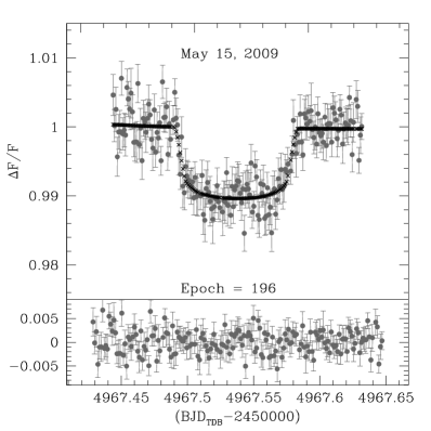
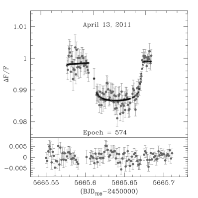
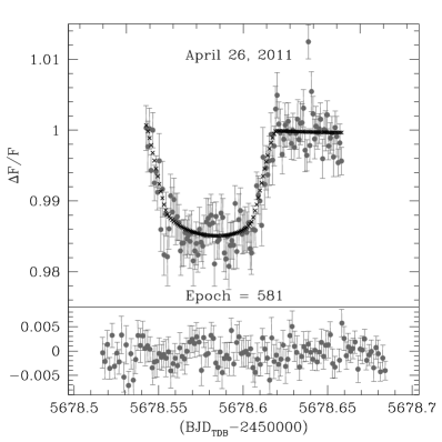
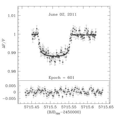
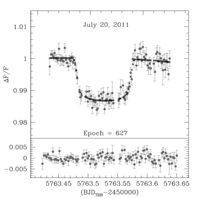
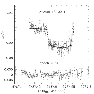
Figure 2: Observed transits of WASP-3b along with our best-fitting models and residuals.

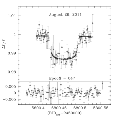
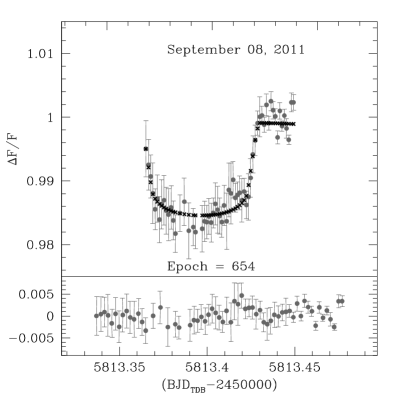
Figure 2: – Continued

In order to further check our ephemerides measurements we applied the barycentric method (Szabó et al. 2006, Oshagh et al. 2012). This technique calculates the transit center ($\rm T_{C}$) as the flux weighted average epoch across the transit:

$$T_{C}\,=\,\frac{\sum_{i=1}^{i=N}\,t_{i}\,(1\,-\,f_{i})}{\sum_{i=1}^{i=N}\,(1\,-\,f_{i})}$$ (5)

where $f_{i}$ is the normalized flux, $t_{i}$ the time and N the total number of measurements within one transit. Transit fitting and barycentric method results agree within 1.9-$\sigma$ (where the $\sigma$ is the average of the uncertainties reported in Table 4) for all the transits with the exception of the transit occurring at epoch 640 (3.7-$\sigma$). In any case, we notice that this transit is almost a partial transit which is at the limit of applicability of the barycentric method.

Table 3: Best-fitting transit parameters.

Date	Epoch ($E$)	Slope ($s$)	Constant ($c$)	$\rm\frac{R_{p}}{R_{s}}$ ($\rm r$)	Duration ($\rm T_{d}$)	Mean stellar density ($\rho_{\star}$)
					(min)	(g$\rm\,cm^{-3}$)
15/05/2009	196	$0.00060_{-0.00060}^{+0.00074}$	$0.99913_{-0.00094}^{+0.00077}$	$0.09506_{-0.00123}^{+0.00309}$	$156.4_{-2.3}^{+4.7}$	$1.05740_{-0.42994}^{+0.02047}$
13/04/2011	574	$-0.00164_{-0.00172}^{+0.00115}$	$1.00068_{-0.00135}^{+0.00203}$	$0.10383_{-0.00110}^{+0.00256}$	$145.4_{-2.6}^{+3.2}$	$1.37746_{-0.45132}^{+0.02257}$
26/04/2011	581	$0.00393_{-0.00268}^{+0.00115}$	$0.99571_{-0.00225}^{+0.00225}$	$0.12177_{-0.00319}^{+0.00172}$	$166.0_{-5.0}^{+5.0}$	$0.51945_{-0.06303}^{+0.25213}$
02/06/2011	601	$0.00078_{-0.00185}^{+0.00123}$	$0.99882_{-0.00153}^{+0.00187}$	$0.10226_{-0.00134}^{+0.00269}$	$162.1_{-2.5}^{+5.0}$	$0.80799_{-0.24422}^{+0.16908}$
20/07/2011	627	$-0.00223_{-0.00106}^{+0.00106}$	$1.00243_{-0.00142}^{+0.00095}$	$0.10904_{-0.00192}^{+0.00128}$	$168.1_{-2.3}^{+3.8}$	$0.82458_{-0.20157}^{+0.09406}$
13/08/2011	640	$-0.00274_{-0.00163}^{+0.00163}$	$1.00208_{-0.00223}^{+0.00149}$	$0.10222_{-0.00166}^{+0.00249}$	$157.8_{-2.0}^{+5.1}$	$1.01379_{-0.35486}^{+0.03735}$
26/08/2011	647	$-0.00080_{-0.00137}^{+0.00150}$	$0.99998_{-0.00175}^{+0.00143}$	$0.10534_{-0.00293}^{+0.00267}$	$147.0_{-4.2}^{+10.4}$	$1.09265_{-0.48430}^{+0.22601}$
08/09/2011	654	$-0.00122_{-0.00308}^{+0.00205}$	$1.00056_{-0.00312}^{+0.00312}$	$0.11422_{-0.00203}^{+0.00304}$	$163.8_{-3.3}^{+5.4}$	$0.95100_{-0.31570}^{+0.05262}$

Table 4: Collection of transit timing measurements of WASP-3b in chronological order.

Epoch	Time of transit minimum	$\Delta^{-}(\rm BJD_{TDB})$	$\Delta^{+}(\rm BJD_{TDB})$	$\rm(O\,-\,C)$	$\Delta^{-}(\rm O\,-\,C)$	$\Delta^{+}(\rm O\,-\,C)$	Reference
	($\rm BJD_{TDB}$-2450000)	(days)	(days)	(sec)	(sec)	(sec)
-250.	4143.85104	0.00040	0.00040	-46.	35.	35.	Pollacco et al. (2008)
-2.	4601.86588	0.00027	0.00027	-44.	23.	23.	Tripathi et al. (2010)
0.	4605.56030	0.00035	0.00035	21.	30.	30.	Gibson et al. (2008)
12.	4627.72172	0.00031	0.00031	-30.	27.	27.	Tripathi et al. (2010)
18.	4638.80403	0.00031	0.00031	83.	27.	27.	Tripathi et al. (2010)
30.	4660.96509	0.00021	0.00021	1.	18.	18.	Tripathi et al. (2010)
40.	4679.43269	0.00050	0.00050	-63.	43.	43.	Christiansen et. al. (2011)
41.	4681.27911	0.00040	0.00040	-99.	35.	35.	Christiansen et. al. (2011)
42.	4683.12740	0.00035	0.00035	27.	30.	30.	Christiansen et. al. (2011)
43.	4684.97486	0.00027	0.00027	81.	23.	23.	Christiansen et. al. (2011)
44.	4686.82053	0.00059	0.00059	-19.	51.	51.	Christiansen et. al. (2011)
46.	4690.51381	0.00055	0.00055	-53.	48.	48.	Christiansen et. al. (2011)
47.	4692.36117	0.00043	0.00043	-7.	37.	37.	Christiansen et. al. (2011)
48.	4694.20711	0.00042	0.00042	-84.	36.	36.	Christiansen et. al. (2011)
59.	4714.52284	0.00036	0.00036	-36.	31.	31.	Gibson et al. (2008)
194.	4963.84436	0.00072	0.00072	-128.	62.	62.	Tripathi et al. (2010)
194.	4963.84563	0.00055	0.00055	-18.	48.	48.	Sada et al. (2012)
196.	4967.53651	0.00057	0.00085	-259.	49.	73.	This work
201.	4976.77365	0.00051	0.00051	-3.	44.	44.	Tripathi et al. (2010)
236.	5041.41271	0.00049	0.00049	-14.	42.	42.	Maciejewski et al. (2010)
249.	5065.41995	0.00059	0.00059	-152.	51.	51.	Maciejewski et al. (2010)
256.	5078.34873	0.00058	0.00058	-71.	50.	50.	Maciejewski et al. (2010)
269.	5102.35933	0.00056	0.00056	81.	48.	48.	Maciejewski et al. (2010)
289.	5139.29713	0.00049	0.00049	178.	42.	42.	Maciejewski et al. (2010)
379.	5305.51082	0.00039	0.00039	60.	34.	34.	Maciejewski et al. (2010)
403.	5349.83457	0.00039	0.00039	37.	34.	34.	Sada et al. (2012)
403.	5349.83182	0.00039	0.00039	-200.	34.	34.	Sada et al. (2012)
404.	5351.68320	0.00110	0.00110	192.	95.	95.	Littlefield (2011)
430.	5399.69990	0.00150	0.00150	108.	130.	130.	Littlefield (2011)
436.	5410.78020	0.00130	0.00130	47.	112.	112.	Littlefield (2011)
450.	5436.63590	0.00080	0.00080	49.	69.	69.	Littlefield (2011)
456.	5447.71550	0.00080	0.00080	-72.	69.	69.	Littlefield (2011)
574.	5665.64627	0.00069	0.00056	305.	60.	48.	This work
581.	5678.57065	0.00106	0.00087	6.	92.	75.	This work
592.	5698.88358	0.00060	0.00060	-188.	52.	52.	Sada et al. (2012)
601.	5715.50608	0.00074	0.00060	-102.	64.	52.	This work
627.	5763.52552	0.00070	0.00047	50.	60.	41.	This work
640.	5787.53379	0.00080	0.00080	1.	69.	69.	This work
647.	5800.46112	0.00113	0.00170	-43.	98.	147.	This work
654.	5813.38792	0.00098	0.00080	-133.	85.	69.	This work

6 Radial velocities

Radial velocities can be used together with transit timing variations to place more stringent constrains on the presence of a perturbing object in the WASP-3b system. We therefore gathered all the radial velocity measurements of WASP-3b publically available from the Exoplanet Orbit database. These measurements were presented in Pollacco et al. (2008), Simpson et al. (2010) and Tripathi et al. (2010) and in the following we first introduced in more detail these datasets.

6.1 Available data sets

Pollacco et al (2008) obtained seven radial velocity measurements of WASP-3 using the SOPHIE spectrograph at the 1.93-m telescope at Haute-Provence Observatory. The observations were performed between 2007 July 2-5 and August 27-30. All the measurements were acquired outside the transit. Simpson et al. (2010) acquired 26 spectra of WASP-3 during the transit occurring on the night of 2008 September 30. The observations were also obtained with the SOPHIE spectrograph at the 1.93-m telescope at Haute-Provence Observatory. These authors also reanalysed the seven measurements presented in Pollacco et al. (2008) based on an updated version of the SOPHIE pipeline. We therefore decided to use these data in our study and not the original data presented in Pollacco et al. (2008).

Figure 3: Observed minus calculated times of transit minimum. Filled circles denote previous literature results, open circles the new measurements presented in this work.

Tripathi et al. (2010) obtained 33 radial velocity measurements of WASP-3b with the High Resolution Spectrometer (HIRES; Vogt et al. 1994) on the Keck I 10 m telescope at the W. M. Keck Observatory on Mauna Kea. The observations were acquired both during the transit (on 2008 June 19, 21 and on 2009 June 3) and outside the transit on several other nights in 2008 and 2009.

7 Analysis of the radial velocity data

We analyzed simultaneously all the radial velocity measurements presented both by Tripathi et al. (2010) and Simpson et al. (2010). Since many measurements were acquired during the transit, we fit the data with a model describing both the Keplerian motion of the host star and the Rossiter-McLaughlin anomaly. On one hand we modeled the Keplerian motion as:

$$RV\,=\,\tilde{K}\frac{\cos u+k}{\sqrt{1-h^{2}-k^{2}}}+\gamma$$ (6)

where $\tilde{K}$ is the radial velocity semi-amplitude without the contribution of the eccentricity $e$, $k=e\,\cos\omega$, $h=e\,\sin\omega$, $\gamma$ is the barycentric radial velocity and $u=\nu+\omega$ is the true argument of latitude with $\nu$ the true anomaly and $\omega$ the argument of the pericenter.

On the other hand we accounted for the Rossiter-McLaughlin (RM) anomaly following Hirano et al. (2010) but including an improved treatment of the RM effect during the partial phases of the transit (as detailed in Appendix B):

$$RV_{RM}\,=-df\,\times\,v_{p}\,\Big{[}p-q\,\Big{(}\frac{v_{p}}{v\sin i}\Big{)}^{2}\Big{]}$$ (7)

where $df$ is the flux loss due to the transit of the planet in front of the disk of the star, which we modeled as in Mandel & Agol (2002), $p$ and $q$ are two parameters related to modellization of the Rossiter-McLaughlin effect as proposed by Hirano et al. (2010) and were fixed to the values adopted by Tripathi et al. (2010) and Simpson et al. (2010) as reported in Table 5, $v_{p}$ is the average velocity of the star below the area occulted by the planet (Hirano et al. 2010 and Appendix B), and $v\sin i$ is the rotation velocity of the star.

Table 5: Adopted values for the $p$ and $q$ parameters and for the limb darkening coefficients entering in the Rossiter-McLaughlin model.

$p$	$q$	$g_{1}$	$g_{2}$	Reference
1.51	0.44	0.596	0.215	Tripathi et al. (2010)
1.72	0.00546	0.69	0.	Simpson et al. (2010)

We considered as free parameters: $\tilde{K}$, $h$, $k$, $\lambda$ (the spin-orbit angle), $v\sin i$, and $\gamma$. Both Tripathi et al. (2010) and Simpson et al. (2010) distinguished two different groups of data in their own dataset to account for possible systematic radial velocity variations during their observing runs. We decided to perform the fit twice, first following the analysis of those authors and therefore allowing for a total number of four different barycentric radial velocities. Then, we redid the fit considering only two different barycentric radial velocities for the Tripathi et al. (2010) and Simpson et al. (2010) datasets. This second approach was intended to check for possible long-term variations among the RV residuals that could have been canceled out by the adoption of a larger number of free parameters. Then, in the end, we considered either nine or seven free parameters for the two fits respectively. We notice that Tripathi et al. (2010) excluded from the fit three data points which were presenting a clearly deviant radial velocity with respect to the remaining measurements. This radial velocity $spike$ was ultimately attributed by the authors to residual moonlight unexpectedly leaking into the spectrograph and therefore we neglected them hereafter. Additionally Tripathi et al. (2010) added in quadrature to the uncertainties of their data a value equal to 14.8$\rm\,m\,s^{-1}$ to account for jitter noise. Since, however, it is not clear which is the origin of this noise, we didn’t apply this correction.

The convergence toward the best-fit solution was obtained by means of a Levenberg-Marquardt algorithm, and the uncertainties and the best fit values of the parameters by means of a Markov Chain Monte Carlo analysis as done for the photometric data. The radial velocity measurements after subtraction of the barycentric velocities, along with the best fit model and distinguished in the four (two) different groups of data to which the different $\gamma$ were applied are shown in Fig. 4 (upper panels). The result after the subtraction of the RM anomaly is shown in the middle panels of Fig. 4, and the residual velocities after subtracting the Keplerian orbit also are shown in the bottom panels. Our best-fit parameters are given in Table 6 along with the values obtained by other authors. Our best-fit model corresponds to a $\sqrt{\chi_{r}^{2}}=1.5$ for the four $\gamma$ solution and to $\sqrt{\chi_{r}^{2}}=1.6$ for the two $\gamma$ solution. Our results are in agreement with the literature values. The barycentric velocities for the case of the four $\gamma$ solution are consistent with those derived by Tripathi et al. (2010) and Simpson et al. (2010), and in the case of the 2$\gamma$ solution our values for each dataset are in between the results reported by those authors for their own data. We obtained a value of the spin-orbit angle consistent with zero. We also notice that the rotation velocity we obtained for the four $\gamma$ solution ($\rm v\sin(i)=13.9^{+0.3}_{-0.5}$) is perfectly consistent with the result of Miller et al. (2010) implying $\rm v\sin(i)=13.9^{+0.03}_{-0.03}$. For the two $\gamma$ solution we obtained instead a larger value of the rotation velocity ($\rm v\sin(i)=14.5^{+0.3}_{-0.3}$).

Table 6: Best-fit parameters obtained from our reanalysis of the radial velocity measurements (TW=This work), and from the study of Simpson et al. (2010, SI10), Tripathi et al. (2010, TR10), Miller et al. (2010, MI10) and Pollacco et al. (2008, PO08).

$v\sin i$	$\lambda$	$\tilde{K}$	$k$	$h$	$\gamma_{1}$	$\gamma_{2}$	$\gamma_{3}$	$\gamma_{4}$	Ref
(km$\rm\,s^{-1}$)	(deg)	(m$\rm\,s^{-1}$)			(km$\rm\,s^{-1}$)	(km$\rm\,s^{-1}$)	(km$\rm\,s^{-1}$)	(km$\rm\,s^{-1}$)
13.9${}^{+0.3}_{-0.5}$	-3${}^{+1}_{-2}$	282${}^{-5}_{+7}$	0.04${}^{+0.02}_{-0.01}$	0.03${}^{+0.01}_{-0.01}$	0.029${}^{+0.007}_{-0.002}$	0.048${}^{+0.003}_{-0.007}$	-5.453${}^{+0.005}_{-0.010}$	-5.483${}^{+0.01}_{-0.007}$	TW (4$\gamma$)
14.5${}^{+0.3}_{-0.3}$	-1.9${}^{+1.4}_{-0.9}$	287${}^{+3}_{-9}$	0.060${}^{+0.009}_{-0.024}$	0.035${}^{+0.007}_{-0.016}$	0.040${}^{+0.003}_{-0.004}$	-	-5.469${}^{+0.007}_{-0.005}$	-	TW (2$\gamma$)
15.7${}^{+1.4}_{-1.3}$	13${}^{+9}_{-7}$	276$\,\pm\,$11	-	-	-	-	-5.458$\,\pm\,0.007$	-5.487$\,\pm\,0.009$	SI10
14.1${}^{+1.5}_{-1.3}$	3.3${}^{+2.5}_{-4.4}$	290.5${}^{+9.8}_{-9.2}$	-	-	0.0335${}^{+0.0063}_{-0.0045}$	0.0476${}^{+0.0062}_{-0.0069}$	-	-	TR10
13.9${}^{+0.03}_{-0.03}$	5${}^{+6}_{-5}$	278.2${}^{+13.8}_{-13.4}$	-	-	-	-	-5.4599${}^{+0.0037}_{-0.0036}$	-	MI10
13.4$\,\pm\,$1.5	-	251.2${}^{+7.9}_{-10.8}$	-	-	-	-	-5.4887${}^{+0.0013}_{-0.0018}$	-	PO08

Figure 4: Radial velocity fit once considering four and two values of $\gamma$ as described in the text (left and right panels respectively). Top panels: radial velocity measurements along with our best fit models. Barycentric radial velocities are subtracted. Middle panels: all radial velocity measurements after subtraction of the barycentric velocities and the Rossiter-McLaughlin anomaly. Lower panels: radial velocity measurements after subtraction of the barycentric velocities, the Rossiter-McLaughlin anomaly and the Keplerian orbit.

8 Analysis of the (O-C) transit timing diagram

In a first step, we analyse whether or not a quadratic departure from a linear fit is present in the transit timings. This could result from the direct interaction with a perturber on an extended orbit (Borkovits et al. 2011), or from the light travel timing produced by the motion of the star also induced by a hypothetical distant companion (Montalto 2010). This test can be performed following the approach of Pringle (1975) which measures the improvement of a fit by a quadratic parabola with respect to a simpler one by a straight line. However, the quadratic coefficient obtained by least square is already zero within the errorbars $(-0.9\pm 3.5)\,\times 10^{-9}$ days. We thus conclude that there is no significant long term quadratic trend in the data.

Then, we follow the analysis of Maciejewski et al. (2010). We compute a Lomb-Scargle periodogram on the Transit Timing Variation (TTV) signal in order to detect a periodic oscillation that would reflect the perturbation of a close-in undetected body in the system. For that purpose, we use the generalized version (GLS) of the Lomb-Scargle periodogram (Zechmeister & K$\rm\ddot{u}$rster 2009). Basically the GLS fits a sinusoid to the data for each frequency by using the least square method, as the Lomb-Scargle algorithm, but in addition to that it allows for the presence of an additional constant term. False-alarm probabilities (FAP) are estimated by computing GLS periodograms on a large number of sets of artificial observations in which, for each epoch where a transit has been observed, we replace the measured (O-C) by a random value normally distributed around zero with a standard deviation equal to the uncertainty of that point. The number of periodograms containing a peak with an power above a given threshold out of the total number of trials represents our estimation of the FAP for that given threshold.

Fig. 5(a) shows the GLS periodogram obtained when considering only the transits used by Maciejewski et al. (2010, Fig. 3). We obtain a dominant peak at a frequency $f_{\rm TTV}=0.0145$ cycle $P^{-1}$, which corresponds to P$\rm{}_{TTV}\,=\,127$ days and an power of 0.61, as shown by the arrow, in complete agreement with the result of Maciejewski et al. (2010). Nevertheless the false-alarm probability associated to that power is 27$\%$. There is thus more than one chance out of 4 for this peak to be fortuitous. For the sake of completeness, the false-alarm probability thresholds of 0.1, $10^{-2}$, and $10^{-3}$ are represented by three horizontal lines in the two panels of Fig. 5. We did again the same analysis with all the data of the table 4. The results are displayed in Fig. 5(b). In that case, the peak with the highest power is now at $f_{\rm TTV}=0.0201$ cycle $P^{-1}$ with a FAP equal to 56$\%$. It thus seems that the TTV signal does not contain any significant periodic oscillations.

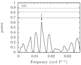
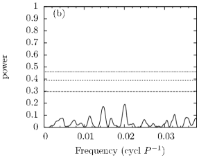
Figure 5: Periodograms of the TTV signal. (a) Considering only the data used in Maciejewski et al. 2010. (b) Using all the data present in Tab. 4. The horizontal lines (from bottom to top) give the FAP thresholds 0.1, $10^{-2}$, and $10^{-3}$.

9 Analysis of the (O-C) radial velocity diagram

We initially checked for the presence of either a linear or a quadratic term in the (O-C) radial velocity residuals by using the Pringle (1975) test. We considered the 2$\gamma$ solution and obtained that in both cases the coefficients are consistent with zero ($0.00001\,\pm\,0.00012$ for the quadratic term) and ($-0.030\,\pm\,0.035$ for the linear term).

A GLS periodogram was then computed. We considered initially the case of the residuals obtained fitting the 4$\gamma$ solution (Sect. 7). As seen in Fig. 6, no significant peaks can be found in the periodogram. The highest peak is at 0.35 days and has a FAP of 31$\%$. Alternative, considering the residuals obtained by the 2$\gamma$ solution, we obtained the highest peak at 0.36 days with a FAP=39$\%$. The FAP of the peaks are estimated with a bootstraping method in the same way as in the previous section. The only difference is that the artificial data are made by shuffling (with repetition) the residuals instead of drawing random values from a normal distribution.

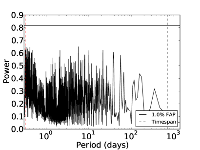
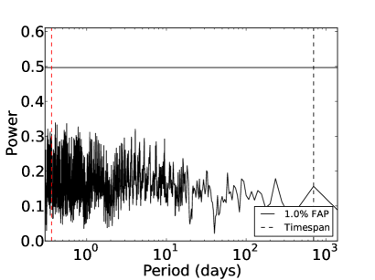
Figure 6: Periodogram of the radial velocity residuals considering the 4$\gamma$ solution (left) and the 2$\gamma$ solution (right). The continuous line denotes the 1$\%$ FAP while the dashed line the time-span of the observations.

10 Discussion

Since the TTV signal does not present any long term variations, nor short period oscillations, one cannot assert that the system actually contains an additional planet. And, if such a companion does exist, its orbital parameters and its mass are poorly constrained due to the lack of expected patterns in the current available data. Nevertheless, the residuals of the fit are quite large ($\sqrt{\chi_{r}^{2}}\simeq 2.30$ and $\sqrt{\chi_{r}^{2}}\simeq 1.5$ for transit and RV respectively). As noticed also by other investigators in the past these values do not indicate a satisfactory fit to the (O-C). The model is thus not complete. Several causes can be at the origin of this result among which we consider here stellar activity, the presence of an additional planet or exomoon and underestimated timing uncertainties.

10.1 Stellar activity

A possible source of TTVs can be the activity of WASP-3. Indeed, the existence of spots on the surface of the star, partially covered by the planet during transits, should produce fluctuations in the luminosity leading to some errors in the determination of the times of transit minimum (e. g. Sanchis-Ojeda et al. 2011; Oshagh et al. 2012). Moreover, the spots, if they exist, should not be the same between the beginning and the end of the observations given the long time span that has been covered ($\sim 4.5$ years). This would explain why no periodic oscillation is detected. Tripathi et al. (2010) reported fractional transit depth variations of the order of $7\%$, even if the same authors were not confident whether these variations were genuine or due to systematics in their data. In addition, they report a mean logR${}^{{}^{\prime}}_{\rm HK}$=-4.9 from their Keck spectra taken in 2008-2009.

On the other hand, we reanalysed the spectra taken with SOPHIE. From the 2007 observations (Pollacco et al. 2008) we derived a $\log{\rm R}^{{}^{\prime}}_{\rm HK}$ value of -4.95, whereas the 2009-2010 observations (Simpson et al. 2010) provided a higher value for the activity index of $\log{\rm R}^{{}^{\prime}}_{\rm HK}$=-4.80. Therefore it appears that the mean activity level of the star changed during these years approaching an active phase in 2010. Once considering also the upper limit on the stellar age and the rotation period reported by Miller et al. (2010, age$<2$ Gyr and $\rm P_{rot}=$ 4.3 days) the presence of active regions on this star may not appear a rare circumstance. Despite no clear evidence of starspots crossing has been reported yet, this analysis clearly claims for a more intensive monitoring of the activity level of WASP-3 in order to understand its impact on photometric and radial velocity measurements.

10.2 Additional planet

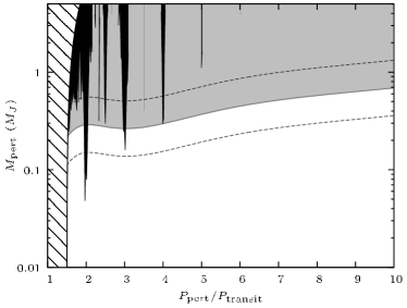
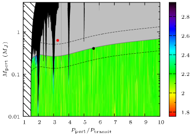
Figure 7: Left: constraints on the maximal mass of a perturber: 99$\%$ confidence detection limits from periodograms of transit timing (black) and radial velocity data (grey). The dashed lines denotes the uncertainty range of the radial velocity detection region. The hatched lines indicates unstable orbits. Right: reduced $\sqrt{\chi^{2}_{r}}$ values resulting from the fit of the observed O-C timing residuals with our model. The calculation is extended over the radial velocity undetectability region, but we also show the regions that produce a $3\,\sigma$ in black. Notice that these regions overlap with the transit timing detectability regions of the left panel.

We now give some constraints on the mass of a hypothetical planetary perturber. For that, we use both the dispersion of the O-C radial velocity and photometric diagrams. For what concerns the radial velocity residuals we adopted here the results coming from the 2$\gamma$ solution, since no significant difference was found adopting instead the 4$\gamma$ solution.

10.2.1 Radial velocities

In the literature, two main approaches are used to find the detection limits in radial velocity data. One is based on $\chi^{2}$- and $F$-tests (e.g. Lagrange et al. 2009, Sozzetti et al. 2009), another is based on a periodogram analysis (Cumming, Marcy & Butler 1999, Endl et al. 2001, Cumming 2004, Narayan, Cumming & Lin 2005). Here, the second approach was chosen due to the number of measurements which is considered high enough for a reliable periodogram analysis.

For each period, a fake eccentric planetary signal is inserted in the data, while the original data is treated as random noise. On these new RV series, the power (in the periodogram) is calculated. The semi-amplitude of the fake signal is changed untill the FAP level is reached for all eccentricities $e$, times of periastron $T_{c}$ and longitudes of periastron $\varpi$. In this paper, a FAP of $1\%$, determined with $1000$ shuffled time series, is used. Fake signals are tested for periods $P$ between 1 and 20 days. The orbital elements of the eccentric signals range, in 10 steps, as follows: $0\leq e\leq 1$, $0\leq T_{c}\leq P$ and $0\leq\varpi\leq 2\pi$. The final semi-amplitude can be transformed in planetary mass and expresses the lower limit for detectable planets at that period with these data.

$$M_{p}\sin i=1.2\cdot 10^{-3}K\sqrt{1-e^{2}}\left(\frac{PM_{\ast}^{2}}{2\pi G}\right)^{1/3}$$ (8)

with the planetary mass in Earth mass, the semi-amplitude $K$ in m/s, the period $P$ in days, the stellar mass $M_{\ast}$ in solar masses and the gravitational constant $G$ in m³kg^-1s^-2. Therefore the continuous grey line in Fig. 7 denotes the limit in the perturber mass beyond which a signal would have been detected in the radial velocity data with a confidence limit equal to $99\%$. The dashed lines shows the 1-$\sigma$ uncertainty range of the radial velocity detection limit.

10.2.2 Photometry

We exclude compact systems which lead to unstable evolutions. Only circular and coplanar systems have been considered since they provide the strongest constraints and because the projected spin-orbit angle measure on WASP-3b by the Rossiter-McLaughlin effect is compatible with zero as demonstrated above, suggesting that if a planetary companion exists, the system is likely coplanar.

The radial velocity measurements are used to exclude any perturbers that would induce RV signal with an amplitude larger than the 1$\%$ FAP threshold. The same exercise has been performed with the O-C of the transit timing measurements. For that, we simulated a large number of O-C on a grid of parameters of the perturber. We considered 400 periods $P_{\rm pert}$ ranging between 1.5 and 10 $P_{\rm transit}$ (where $P_{\rm transit}=P$ is the period of the transiting planet), and 100 masses $M_{\rm pert}$ evenly distributed in logarithm between 0.01 and 5 $M_{J}$. For each period and mass, 60 simulations are performed with different initial longitudes between 0 and 360^∘. Among the 60 simulations, the one giving the periodogram with the lowest maximum amplitude is kept. If this amplitude is above the 1$\%$ FAP threshold determined in section 8, then the corresponding perturber should have been detected in the periodogram of the O-C (see Fig. 5), otherwise the perturber can exist but it is not detectable.

Figure 7 (left) shows the results. The hatched region, which extends up to a period ratio of 1.5, delineates the chaotic orbits which are excluded. The boundary of this region has been derived from the stability criterion of (Gladman 1993). The gray curve fixes the limit of the perturber’s mass from the radial velocity measurements. Any perturber in the gray region would induce a periodic RV signal with a significant amplitude. And finally, the black regions delineate the perturbers that produce TTVs with significant oscillating terms. Combining all the information, it turns out that the radial velocity technique excludes any perturber as massive as Jupiter up to a period ratio of 10, and the TTV measurements provide stronger constraints close to mean motion resonances.

In a second step, we focused on perturbers that do not produce any significant periodic RV signals nor periodic TTV signals. Such perturbers are located in the white region of Fig. 7 (left). For those perturbers, we check whether they can reproduce the O-C transit timing diagram or not. In that purpose, we use the same grid of parameters as in Fig. 7 (left), and for each initial conditions, we compute the expected TTVs and the reduced chi-square with respect to the observations. The results are displayed in Fig. 7 (right). The hached and the gray regions are the same as in Fig. 7 (left). The black regions correspond now to simulated TTVs above the 3-$\sigma$ level. This threshold is obtained from the $\chi^{2}$-distribution with 33 degrees of freedom. It corresponds to $\chi_{r}^{2}=\chi_{r,\rm min}^{2}(1+1.821)$, or $\sqrt{\chi_{r}^{2}}=2.95$. The colour scale represents the $\sqrt{\chi_{r}^{2}}$ from the lowest values in red up to the 3-$\sigma$ threshold in dark violet. The red circle shows the best fit to the observation with $\sqrt{\chi_{r}^{2}}=1.76$. However, such a perturber, with a mass of 0.63 $M_{J}$ should have been detected in the radial velocity analysis. The best fit within the undetectable perturbers is just below the RV detection threshold with $M_{\rm pert}=0.41M_{J}$ and $P_{\rm pert}=5.63P_{\rm transit}$, but the corresponding reduced chi-square is only $\sqrt{\chi_{r}^{2}}=1.83$. The improvement is very weak. Moreover, from Fig. 7 (right), one can see that such values of the reduced chi-square are spread more or less randomly within the undetectable region.

As noted by Maciejewski et al. (2010), the presence of an outer companion less massive than WASP-3b but still on a short period orbit would make the system quite unusual. Multiplanetary systems containing at least a Jupiter-mass planet are indeed much wider, and the less massive planet is usually the closest to the star (e. g. Lissauer et al. 2011).

10.3 Exomoon

An exomoon is also supposed to generate a periodic oscillation in the TTV. However, Maciejewski et al. (2010) have already discarded this hypothesis since the transits do not show any duration variations shifted in phase by $\pi/2$ with respect to the timing variations. Here, we perform a more detailled analysis based on the results of Kipping (2009).

First of all, we check that an exomoon can have a stable orbit. If the moon is less than twice as dense as the planet the minimum distance of the moon is set by the Roche limit. Let $\xi$ be the semi-major axis of a hypothetical satellite divided by the Hill Radius, i.e. $a_{s}=\xi R_{H}$ where $a_{s}$ is the semi-major axis of the moon and $R_{H}$ the Hill Radius. According to Kipping (2009), $\xi$ should satisfy the following inequality

$$\chi_{\rm min}\lesssim\xi\lesssim\frac{1}{3}\ ,$$ (9)

where $\xi_{\rm min}=1/186\times(M_{s}/M_{\oplus})^{-0.063}(P/1{\rm d})^{-2/3}$ represents the Roche limit. In this expression, $M_{s}$ is the mass of the satellite and $P$ is the orbital period of the planet. For an exomoon of the mass of the Earth’s Moon, we get $\xi_{\rm min}=0.0047$, and for an exomoon of the mass of the Earth, $\xi_{\rm min}=0.0036$. In both cases $\chi_{\rm min}$ is lower than $1/3$. For moons which density is more than twice that of the planet the Roche limit would be inside the planet, therefore the minimum distance would correspond to the planetary radius and the above inequality would be automatically satisfied. Therefore an exomoon can exist on a stable orbit around WASP-3.

Then, we estimate the maximal RMS amplitude ($\delta_{\rm TTV}$) of TTV that an exomoon on a coplanar circular orbit can produce. According to Kipping (2009), this amplitude is given by

$$\delta_{\rm TTV}=\frac{1}{\sqrt{2}}\frac{P}{2\pi}\left(\frac{M_{ps}}{3M_{\star}}\right)^{1/3}\mu(1-\mu)^{1/3}\xi\ ,$$ (10)

with $\mu=M_{s}/M_{ps}$ and $M_{ps}$ is the sum of the planet mass and the satellite mass. Without any constraint on $\mu$, the maximum of the product $\mu(1-\mu)^{1/3}$ is attained for $\mu=3/4$, and is equal to $3/4^{1/3}$. However, by definition, the Moon should have a lower mass than the planet. If the transit lightcurves are those of the planet, $\mu$ should be lower than $1/2$, and probably much lower. But let us assume that $\mu=1/2$, this will provide the upper limit of $\delta_{\rm TTV}$. If the planet has an exomoon, the Keplerian orbit derived in the previous section is that of the planet-satellite barycenter around the star. Thus the fitted mass corresponds to $M_{sp}$. Using $M_{sp}/M_{\star}=1.5\times 10^{-3}$, one obtains

$$\delta_{\rm TTV}\leq\frac{1}{\sqrt{2}}\frac{1}{2^{4/3}}\frac{P}{2\pi}\left(\frac{M_{sp}}{3M_{\star}}\right)^{1/3}\xi=9.4\,\xi\quad{\rm[min]}\ .$$ (11)

For $\xi=\xi_{\rm max}=1/3$, this leads to $\delta_{\rm TTV}\leq 3.1$ min. The result is larger than the observed RMS of the O-C which is equal to 1.1 min. Thus, a “satellite” as massive as the planet ($\mu=1/2$) is able to produce significant TTV with an amplitude comparable to the observed one.

We now assume that the observed O-C is only due to an hypothetical satellite. Expecting that this satellite should have a much smaller mass than the planet, we derive its mass for $\xi=\xi_{\rm max}=1/3$ such that $\delta_{\rm TTV}=1.1$ min. One gets $\mu=0.14$, which corresponds to a mass ratio of $M_{s}/M_{p}=0.17$, or $M_{s}\approx 0.35M_{J}$. Thus, the lowest massive satellite, on circular orbit, that can account for the observed RMS of the O-C is still large. Assuming the same density as a giant planet like Jupiter, the radius of this satellite should be $0.46R_{J}$. Such a big satellite, if it existed, would produce detectable transits in the lightcurve. We also noticed that a search for additional transiting objects in the NASA $EPOXI$ mission WASP-3 lightcurve resulted in a null detection (Ballard et al. 2011). However, we note that accordingly to Domingos et al. (2006) the value of the critical semi-major axis could approach the value of 0.9309 in units of the Hill radius, for retrogade moons. In this case we can obtain a more stringent constraint on the maximum mass of the moon which could be equal to $M_{s}/M_{p}=0.04$ or $M_{s}\approx 0.07\,M_{J}$. In Fig. 8, we also show our transit durations against the O-C residuals. In case of an exomoon being responsible for the claimed TTVs, we should expect the observations to trace an ellipse in this diagram since the TTVs and the TDVs (Transit Duration Variations) produced by an exomoon are shifted in phase by $\pi/2$ (Kipping 2009). For illustration, we overplot the expected signal that the above-mentioned prograde satellite ($M_{s}=0.35M_{J}$ and $\chi=1/3$) should generate. Evidently given the large errorbars of our measurements it is not possible to explore this possiblity, and additional more accurate measurements are required for this analysis.

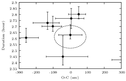
Figure 8: Transit durations against O-C transit timing residuals for the new transits presented in this work. Overplot a representative signal produced by an exomoon having $M_{s}=0.35M_{J}$ and period $\chi=1/3$.

10.4 Underestimated uncertainties

It is difficult to ascertain up to which level different instruments, observing conditions, reduction and transit fitting procedures may affect the results reported in Table 4. To address this point it would be necessary to homogeneously reduce and analyze all the data collected so far by all the different groups, an approach which is not easy to put into practice. In principle all the transits considered here were presented in referred journals and this ensures that accurate procedures like those ones reported here have been applied to estimate transit timing errors. It is our opinion however that error underestimation cannot be completely ruled out. New observations will be certainly welcome to clarify this problem.

11 Conclusions

In this work we provided a throughout analysis on the presence of additional bodies in the WASP-3 system. This analysis serves to improve our understanding of close-in Jupiters and in particular to clarify if these planets are indeed isolated or not.

In addition to present eight new transits of WASP-3b acquired at the Crow-Observatory-Portalegre in Portugal we reanalized all the photometric and radial velcocity measurements aquired so far for this system. We concluded that there is no convincing evidence of additional planetary companions in this system; both the transit timing and the radial velocity residuals do not present significant periodicities (FAP=56$\%$ and FAP=$31\%$ for transit and radial velocity in the best case scenario respectively) nor long term trends.

Combining all transit timing and radial velocity informations, we obtained that any perturber more massive than $\rm M\gtrsim 100\rm M_{\oplus}$ and with period up to ten times the period of the inner planets is excluded at 99$\%$ confidence limit.

We also investigated the possible presence of an exomoon on this system and determined that considering the scatter of the O-C transit timing residuals a coplanar exomoon would likely produce detectable transits, an hypothesis that can be ruled out by observations conducted by other researchers. In case the orbit of the moon is not complanar the current accuracy of transit timing and transit duration measurements prevents to make any significant statement. For retrogade moons the maximum mass allowed at the critical semi-major axis is around 0.1 $M_{J}$.

Finally on the basis of our reanalysis of SOPHIE data we noted that WASP-3 passed from a less active ( $\log{\rm R}^{{}^{\prime}}_{\rm hk}=-4.95$) to a more active ( $\log{\rm R}^{{}^{\prime}}_{\rm hk}=-4.8$) state between 2007 and 2010. Despite no clear spot crossing has been reported for this system so far we therefore pointed out the need for a more intensive monitoring of the activity level of this star in order to understand its impact on photometric and radial velocity measurements.

Our lightcurves are made available through the on-line version of this journal.

Appendix A: the normalized planet distance

Here we derive the expression for the normalized planet distance $z$ presented in Eq. 1. Assuming a circular orbit and a constant projected velocity ($v$) of the transiting planet on the plane of the sky, in any given instant $t$ during the transit the normalized distance $z$ can be written as

$$z^{2}\, = \,\Big{(}\frac{b}{R_{\star}}\Big{)}^{2}\,+\,\Big{(}v\,\frac{t-T_{0}}{R_{\star}}\Big{)}^{2},$$

where $b$ is the impact parameter, $R_{\star}$ is the radius of the star and $T_{0}$ is the time of transit minimum. At the time of the first or the fourth contact we have

$$z^{2}\,=\,(r+1)^{2} = \Big{(}\frac{b}{R_{\star}}\Big{)}^{2}\,+\,\Big{(}v\,\frac{T_{d}}{2\,R_{\star}}\Big{)}^{2},$$

where $r$ is the ratio of the radius of the planet to the radius of the star, and $T_{d}$ is the total transit duration (from the first to the fourth contact). Assuming the projected velocity during the transit to be identical to the orbital velocity we can write

$$v = \sqrt{\frac{G\,M_{\star}}{a}},$$

where $G$ is the gravitational constant, $M_{\star}$ is the mass of the star, $a$ is the semi-major axis and we neglected the mass of the planet. Eliminating in the first equation above the impact parameter derived from the second, using the third Kepler law and introducing the definition of the mean stellar density

$$\rho_{\star} = \frac{M_{\star}}{\frac{4}{3}\pi\,R_{\star}^{3}},$$

we obtain Eq. 1:

$$z^{2}(t)\, = \Big{(}\frac{8\,\pi^{2}\,\rm G}{3\,\rm P}\Big{)}^{2/3}\,\rho_{\star}^{2/3}\,\Big{[}(t-T_{0})^{2}-\Big{(}\frac{T_{d}}{2}\Big{)}^{2}\Big{]}\,+$$

$$+ \,(1\,+\,r)^{2}.$$

Appendix B: RM effect during the ingress and the egress

In this Appendix we introduce a new analytic representation of the Rossiter-McLaughlin effect valid during the ingress and the egress of the transit, that is between the first to the second contact and between the third to the fourth contact. During these phases the formula presented by Hirano et al. (2010) accounts for the velocity of the star below the disk of the planet considering the value of the velocity at the center of the disk of the planet, and it is therefore valid for the small planets approximation. We instead integrated the velocity profile below the disk and calculated the average velocity which makes our approach consistent with the calculation of Hirano et al. (2010) for the remaining phases of the transit. This derivation is based on the method described in (Pál 2012).

Therefore if we define X and Y as the coordinates of the center of the planet at a given instant during the transit, accordingly to the choice of parameters we adopted in this paper we have

Figure 9: Definition of the $\psi_{0}$, $\phi_{0}$, $\epsilon$ and $\xi$ angles introduced in the text.

$$X = \frac{(1-e\,\sin\omega)}{\sqrt{1-e^{2}}}\Big{(}\frac{8\pi^{2}G}{3P}\Big{)}^{1/3}\,\rho^{1/3}_{\star}\,(t-T_{0})\ ,$$

$$Y = \frac{(1-e\,\sin\omega)}{\sqrt{1-e^{2}}}\sqrt{(1+r)^{2}-\Big{(}\frac{8\pi^{2}G}{3P}\Big{)}^{2/3}\,\rho^{2/3}_{\star}\Big{(}\frac{T_{d}}{2}\Big{)}^{2}}\ .$$

Then if $\lambda$ is the spin-orbit angle projected on the plane of the sky, in the rotated coordinate system which vertical axis is aligned with the projected spin axis of the star, the coordinates x and y are given by

$$x = X\cos\lambda-Y\sin\lambda\ ,$$

$$y = X\sin\lambda+Y\cos\lambda\ .$$

Let $\psi_{0}$, $\phi_{0}$, $\epsilon$ and $\xi$ be defined as in Fig. LABEL:fig:coordinates with respect to the xy rotated coordinate system, then

$$\psi_{0}\, = \,\rm atan_{2}(y,x)\ ,$$

$$\phi_{0}\, = \,\psi_{0}\,+\,\pi\ .$$

Assuming that the radius of the star is normalized to unity, one gets

$$\epsilon\, = \,\rm acos\Big{(}\frac{1-r^{2}+z^{2}}{2\,z}\Big{)}\ ,$$

$$\xi\, = \,\rm acos\Big{(}\frac{r^{2}+z^{2}-1}{2\,r\,z}\Big{)}\ ,$$

where

$$z\, = \,\sqrt{x^{2}+y^{2}}\ .$$

Defining now the angles $\psi_{a}$, $\psi_{b}$, $\phi_{a}$ and $\phi_{b}$ as

$$\psi_{a}\, = \psi_{0}\,-\,\epsilon\ ,$$

$$\psi_{b}\, = \psi_{0}\,+\,\epsilon\ ,$$

$$\phi_{a}\, = \phi_{0}\,-\,\xi\ ,$$

$$\phi_{b}\, = \phi_{0}\,+\,\xi\ ,$$

and defining the following functions

$$A(\alpha,\beta,\gamma) = \frac{1}{2}\alpha^{2}\beta\sin\gamma+\frac{1}{2}\alpha\beta^{2}\left(\gamma+\frac{1}{2}\sin 2\gamma\right)$$

$$+ \frac{1}{2}\beta^{3}\left(\gamma+\frac{1}{3}\sin^{3}2\gamma\right)\ ,$$

$$B(\alpha,\beta,\gamma) = \frac{1}{2}\alpha\beta\sin\gamma+\frac{1}{2}\beta^{2}\left(\gamma+\frac{1}{2}\sin 2\gamma\right)\ ,$$

the subplanet velocity $v_{p}$ is given by

$$\frac{v_{p}}{v\sin i}\, = \,\frac{A_{\rm tot}}{B_{\rm tot}}$$

where

$$A_{\rm tot} = A(0,1,\psi_{b})-A(0,1,\psi_{a})+A(x,r,\phi_{b})-A(x,r,\phi_{a})\ ,$$

$$B_{\rm tot} = B(0,1,\psi_{b})-B(0,1,\psi_{a})+B(x,r,\phi_{b})-B(x,r,\phi_{a})\ .$$

During the full transit pahse, Eq. 10 reduces to

$$\frac{v_{p}}{v\sin i} = x\ ,$$

which is equal to Eq. A8 of Hirano et al. (2010).

References

- Ballard et al. (2011) Ballard S. et al., 2011, ApJ, 732, 41
- Borkovits et al. (2011) Borkovits T., Csizmadia Sz., Forgács-Dajka E., Hegeds T., 2011, A&A, 528, 53
- Claret et al. (2011) Claret A., Bloemen S., 2011, A&A, 529, 75
- Charbonneau et al. (2000) Charbonneau D., Brown T. M., Latham D. W., Mayor M., 2000, ApJ, 529, 45
- Chatterjee et al. (2008) Chatterjee S., Ford E. B., Matsumura S., Rasio F. A., 2008, ApJ, 686, 580
- Christiansen et al. (2011) Christiansen J. L. et. al., 2011, ApJ, 726, 94
- Cumming et al. (1999) Cumming A., Marcy G. W., Butler R. P., 1999, ApJ, 526, 890
- Cumming (2004) Cumming A., 2004, MNRAS, 354, 1165
- Domingos et al. (2006) Domingos R. C., Winter O. C., Yokoyama T., 2006, MNRAS, 373, 1227
- Eastman et al. (2010) Eastman J., Siverd R., Gaudi B. S., 2010, PASP, 122, 935
- Endl et al. (2001) Endl M., Krster M., Els S., Hatzes A. P., Cochran W. D., 2001, A&A, 374, 675
- Fabricky et al. (2007) Fabrycky D., Tremaine S., 2007, ApJ, 669, 1298
- Gazak et al. (2012) Gazak J. Z., Johnson J. A., Tonry J., Dragomir D., Eastman J., Mann A. W., Agol E., 2012, Adv. Astron., 2012, 30
- Gelman et al. (1992) Gelman A., Rubin D. B., 1992, Stat. Sci., 7, 457
- Gibson et al. (2008) Gibson N. P. et al., 2008, A&A, 492, 603
- Gladman (1993) Gladman B., 1993, Icarus, 106, 247
- Goldreich et al. (1980) Goldreich P., Tremaine S., 1980, ApJ, 241, 425
- Hirano et al. (2010) Hirano T., Suto Y., Taruya A., Narita N., Sato B., Johnson J. A., Winn J. N., 2010, ApJ, 709, 458
- Juric et al. (2008) Jurić M., Tremaine S., 2008, ApJ, 686, 603
- Kipping (2009) Kipping D. M., 2009, MNRAS, 392, 181
- Kozai (1962) Kozai Y., 1962, AJ, 67, 591
- Kurucz (1993) Kurucz R. L., 1993, ASP Conf. Ser. Vol. 44 P. 87 Astron. Soc. Pac., San Francisco. Title, Peculiar versus Normal Phenomena in A-type and Related Stars, Editors, M. M. Dworetsky, F. Castelli, R. Faraggiana
- Lagrange et al. (2009) Lagrange A.-M., Desort M., Galland F., Udry S., Mayor M., 2009, A&A, 495, 335
- Lissauer (2011) Lissauer J. J. et al., 2011, ApJS, 197, 8
- Littlefield (2011) Littlefield C., 2011, preprint (arXiv1106.4312L)
- Maciejewski et al. (2010) Maciejewski G. et al., 2010, MNRAS, 407, 2625
- Mandel et al. (2002) Mandel K., Agol E., 2002, ApJ, 580, 171
- Mayor et al. (1995) Mayor M., Queloz D., 1995, Nat, 378, 355
- McLaughlin (1924) McLaughlin D. B., 1924, ApJ, 60, 22
- Miller et al. (2010) Miller G. R. M. et al., 2010, A&A, 523, 52
- Montalto (2010) Montalto M., 2010, A&A, 521, 60
- Nagasawa et al. (2008) Nagasawa M., Ida S., Bessho T., 2008, ApJ, 678, 498
- Narayan et al. (2005) Narayan R., Cumming A., Lin D. N. C., 2005, ApJ, 620, 1002
- Nelson et al. (2000) Nelson R. P., Papaloizou J. C. B., Masset F., Kley W., 2000, MNRAS, 318, 18
- Oshagh et al. (2012) Oshagh M., Boué G., Haghighipour N., Montalto M., Figueira P., Santos N. C. 2012, A&A, 540, 62
- Pal (2008) Pál A., 2008, MNRAS, 390, 281
- Pal (2008) Pál A., 2012, MNRAS, 420, 1630
- Pollacco et al. (2008) Pollacco D. et al., 2008, MNRAS, 385, 1576
- Pont et al. (2006) Pont F., Zucker S., Queloz D., 2006, MNRAS, 373, 231
- Pringle (1975) Pringle J. E., 1975, MNRAS, 170, 633
- Rossiter (1924) Rossiter R. A., 1924, ApJ, 60, 15
- Press et al. (1992) Press W. H., Teukolsky S. A., Vetterling W. T., Flannery B. P., 1992, Cambridge: University Press, c1992, 2nd ed.
- Sada et al. (2012) Sada P. V. et al., 2012, PASP, 124, 212
- Sanchis-Ojeda et al. (2011) Sanchis-Ojeda R., Winn J. N., Holman M. J., Carter J. A., Osip D. J., Fuentes C. I., 2011, ApJ, 733, 127
- Santos et al. (2004) Santos N. C., Israelian G., Mayor M., 2004, A&A, 415, 1153
- Simpson et al. (2010) Simpson E. K. et al., 2010, MNRAS, 405, 1867
- Sneden (1973) Sneden C., 1973, ApJ, 184, 839
- Sousa et al. (2007) Sousa S., Santos N. C., Israelian G., Mayor M., Monteiro M. J. P. F. G., 2007, A&A, 469, 783
- Sousa et al. (2010) Sousa S., Alapini A., Israelian G., Santos N. C., 2010, A&A, 512, 13
- Sozzetti et al. (2007) Sozzetti A., Torres G., Charbonneau D., Latham D. W., Holman M. J., Winn J. N., Laird J. B., O’Donovan F. T., 2007, ApJ, 664, 1190
- Sozzetti et al. (2009) Sozzetti A., Torres, G., Latham D. W., Stefanik R. P., Korzennik S. G., Boss A. P., Carney B. W., Laird J. B., 2009, ApJ, 697, 544
- Stetson (1987) Stetson, P. B. 1987, PASP, 99, 191
- Stetson (1994) Stetson, P. B. 1994, PASP, 106, 250
- Szabo (2006) Szabó Gy. M., Szatmáry K., Divéki Zs., Simon A., 2006, A&A, 450, 395
- Triaud et al. (2010) Triaud A. H. M. J. et al., 2010, A&A, 524, 25
- Tripathi et al. (2010) Tripathi A. et al., 2010, ApJ, 715, 421
- Vogt et al. (1994) Vogt S. S. et al., 1994, SPIE, 2198, 362
- Weidenschilling et al. (1996) Weidenschilling S. J., Marzari F., 1996, Nat, 384, 619
- Wu et al. (2003) Wu Y., Murray N., 2003, ApJ, 589, 605
- Zechmeister et al. (2009) Zechmeister M., Krster M., 2009, A&A, 496, 577