Basic parameters and properties of the rapidly rotating magnetic helium strong B star HR 7355

Abstract

The spectral and magnetic properties and variability of the B2Vnp emission-line magnetosphere star HR 7355 were analyzed. The object rotates at almost 90% of the critical value, meaning it is a magnetic star for which oblateness and gravity darkening effects cannot be ignored any longer. A detailed modeling of the photospheric parameters indicate that the star is significantly cooler than suggested by the B2 spectral type, with R${}_{\rm eff}=17\,500$ K atypically cool for a star with a helium enriched surface. The spectroscopic variability of helium and metal lines due to the photospheric abundance pattern is far more complex than a largely dipolar, oblique magnetic field of about 11 to 12 kG may suggest. Doppler imaging shows that globally the most He enriched areas coincide with the magnetic poles and metal enriched areas with the magnetic equator. While most of the stellar surface is helium enriched with respect to the solar value, some isolated patches are depleted. The stellar wind in the circumstellar environment is governed by the magnetic field, i.e. the stellar magnetosphere is rigidly corotating with the star. The magnetosphere of HR 7355 is similar to the well known $\sigma$ Ori E: the gas trapped in the magnetospheric clouds is fairly dense, and at the limit to being optically thick in the hydrogen emission. Apart from a different magnetic obliquity, HR 7355 and the more recently identified HR 5907 have virtually identical stellar and magnetic parameters.

1 Introduction

The helium-strong star HR 7355 (Rivinius et al. 2008) has recently been found to host a magnetic field with several kilogauss longitudinal strength ($<B_{Z}>$) (Rivinius et al. 2010; Oksala et al. 2010). The rotational period of $P=0.52$ d puts it among the shortest period non-degenerate magnetic stars known, while its $v\sin i\approx 310$ km s ^-1 is the highest for any known non-degenerate magnetic star.

For a long time, rapid rotation (the term “rapid rotation” used here as being at a fraction of well above 50% of break-up velocity) and the presence of a strong magnetic field have been regarded as mutually exclusive for early type stars, and so the sheer existence of this object poses a number of puzzling questions. Most important is the stellar age vs. the expected spin down time. Age estimates for HR 7355 range from 15 to 25 Myr (Mikulášek et al. 2010), much longer than the same authors give for the spin-down timescale, and hence clearly problematic for fossil field explanations. However, the gravity of $\log g=3.95$ found by Oksala et al. (2010) would be more supportive of a younger star. In any case, HR 7355 is a star for which effects like gravity darkening and oblate deformation cannot be ignored. This means traditional analysis methods to derive stellar parameters will, at best, give uncertain results, and at worst misleading ones.

Intriguing is the presence of photospheric abundance nonuniformities, supporting the result that rotational mixing even in rapid rotators should be inhibited at such field strengths (Zahn 2011). Not only are there abundance variations across the stellar surface in HR 7355, but the amplitude of the Hei equivalent width (EW) variations is much larger than in the similar, though less rapidly rotating, Bp star $\sigma$ Ori E.

For the following work we will briefly review the rotational ephemeris in Sect. 1.1, then introduce the new observations in Sect. 2. The first aim of this work is to provide stellar parameters taking into account the rapid stellar rotation, i.e. rotational deformation and gravity darkening, in Sect. 3. The spectroscopic variations are then described and analyzed in detail in Sect. 4, as are the measured properties of the magnetic field in Sect. 5 and of the magnetosphere in Sect. 6. The results are discussed in Sect. 7 and finally the conclusions are drawn in Sect. 8.

1.1 Ephemeris

There are several ephemerides and period determinations, out of which only the one by Rivinius et al. (2008) is clearly obsolete. In order to converge on one, we combined the data used by Rivinius et al. (2010) with the photometric data published by Mikulášek et al. (2010), and the photometric data kindly provided by Oksala et al. (2010). While the period by Rivinius et al. (2010) did not sort well the combined photometric data when phased with this period, the 2008 photometry by Oksala et al. and the 2008/2009 spectroscopy (Rivinius et al. and this work) do have their minima at acommon phase. As a result, we adopt here the epoch given by Rivinius et al. (2010) $T_{0}({\rm MJD})=54\,940.33$, which is the mid-date of an occultation of the star by the magnetospheric material, seen in the Balmer line spectroscopy, and as such very well defined. However, the better period proved to be the value published by Oksala et al., $P=0.5214404(6)$ d, who could rely on a time baseline twice as long. The error of the period is such that for the purposes of this work it can be fully neglected, and we treat the period as a fixed value.

2 Observations

Apart from archival and literature data, which will be referenced where used, this work is based on high-resolution echelle spectra obtained in 2009 with UVES (Dekker et al. 2000) at the 8.2m Kueyen telescope on Cerro Paranal. The instrument was used in the dichroic 2 437/760 setting, which gives a blue spectrum from about 375 to 498 nm and a red spectrum from about 570 to 950 nm, with a small gap at 760 nm. The slit width was 0.8″, giving a resolving power of about $R=50\,000$ over the entire spectrum. The UVES observations were obtained in three service mode observing runs, in April, July, and September 2009 (see Table 1 for the date ranges).

Exposure times were between 120 seconds in April and 30 seconds in July to September, the latter ones being repeated four times in a row. Since the period is short we did not average shorter exposures, but treated them as taken at distinct phases. A few of the blue spectra taken with $t_{\rm exp}=120$ sec were overexposed in better-than-average seeing conditions, thus we have more red than blue spectra. In total, we have 104 blue and 112 red spectra. The typical signal to noise ratio ($S/N$) of a single spectrum is about 275 in the blue region and 290 in the red. However, for unknown reasons, high exposure levels in UVES, even if still in the fully linear regime of the detector, tend to cause some order-merging and global normalization problems, i.e. high $S/N$ data obtained with UVES often have more residual echelle order “wiggles” than data with a lower exposure level. This prompts for local re-normalization of the spectra for analysis of any particular line. In particular, broad spectral features, like Balmer-line wings, are to be treated with care. Our analysis of those features is cross-checked on the low resolution FORS1 long-slit data of Rivinius et al. (2010).

Table 1: Summary of UVES observations

Run	date range		# of spectra
	(MJD)	civil (UT)	blue/red arm
A	54923 – 54951	2009-04-02 to 04-30	29/33
B	55026 – 55062	2009-07-14 to 08-18	55/59
C	55077 – 55083	2009-09-03 to 09-09	20/20

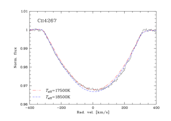
Figure 1: The averaged UVES line profile for Cii$\lambda$ 4267 and the best fitting model for this particular equivalent width, with $T_{\rm eff}=18\,500$ K, and the final best model, taking into account additional conmstraints as discussed in the text, with $T_{\rm eff}=17\,500$ K, both with $v\sin i=310$ km s^-1 and shifted to $v_{\rm sys}=7$ km s^-1.

3 Stellar Parameters

In order to determine the stellar parameters, we made use of spectral synthesis, both for line strength and profiles, as well as for absolute fluxes. The code we used is the third, re-programmed version of Townsend’s (1997) BRUCE and KYLIE suite, which in the following we will call “Bruce3”.

Apart from computational issues, and the implementation of perturbations like pulsation, which is not used here, the main improvement is the treatment of limb-darkening: the code uses either NLTE atmosphere models by Lanz & Hubeny (2007), or Kurucz’s (1992) LTE (ATLAS9) atmospheres, from which the synthetic spectra were computed by SYNSPEC (Hubeny & Lanz 2011), with wavelength-dependent limb-darkening coefficients, i.e. including the effects of limb-darkening on the spectral lines, ranging from 88 to 750 nm. Several characteristics of the line profiles, most notably strengths of Cii and Siii lines in the blue range, were better reproduced with the LTE atmospheres rather than with the NLTE ones (but still using an NLTE spectral profile code). The spectrum of HR 7355 is, therefore, modeled based on an ATLAS9-SYNSPEC grid.

For line-profile comparison, the synthetic spectra, although in principle already “perfectly” normalized (i.e. according to the computed continuum), were re-normalized with the same procedure as the observed spectra, i.e. with a series of smoothly joining spline segments, and using the same wavelengths to sample the continuum.

3.1 Projected rotational velocity and radius

In a first step, the averaged profile of Cii$\lambda$ 4267 was used to obtain the projected rotational velocity by comparing the profile to the grid of Bruce3 models. For any reasonable set of parameters, $v\sin i=310\pm 5$ km s^-1 approximated the width of the observed profile best. We note that this approach completely neglects macroturbulence or other potential broadening mechanisms. However, concerning macroturbulence this is a reasonable approach for a main sequence star, and significant magnetic broadening is not expected for the measured field. The value is in good agreement with Oksala et al. (2010) (see Fig. 1).

The systemic velocity was determined during this measurement as well, to $v_{\rm sys}=7\pm 2$ km s^-1. We found no indication for a variation of this value, hence we can exclude a companion close or massive enough to significantly affect the magnetosphere, unless it would have an orbit in the plane of the sky, i.e. significantly misaligned with the rotation, seen equatorially (see below). Assuming rigid rotation of the circumstellar environment, the derived $v\sin i$ in combination with the rotational period of $P=0.5214404$ d the equatorial radius then becomes $R_{\star,\rm eq}\sin i=3.19\,{\rm R_{\sun}}$. Assuming that a rapidly rotating star is constrained by five independent parameters, usually $v_{\rm eq},i,T_{\rm eff},M_{\star},R_{\star,eq}$, this leaves only three of them to be determined, namely the mass, the effective temperature, and the inclination.

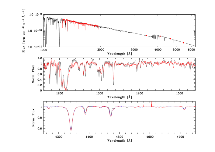
Figure 2: The Bruce3 model (see Table 2) vs. the observed data: Upper panel: SED fit for UV IUE short-wavelength spectrophotometry and Strömgren visual photometry (large red dots) vs. modeled fluxes. Middle panel: Line profile fit for IUE spectrum (red) vs. modeled UV line profiles (black). Lower panel: Line profile fit for averaged UVES (red) and FORS1 (blue) spectra vs. modeled visual line profiles (black). Note that in this step solar abundances are still used, hence the mismatch for the helium profiles. This discrepancy is solved later by the Doppler imaging.

3.2 Effective temperature

The interpretation of the effective temperature $T_{\rm eff}$ in a rapidly rotating star, i.e. in a star where gravity darkening and oblateness have become significant, is not straightforward. So we note that Bruce3 uses $T_{\rm eff}$ in the sense that it is the uniform temperature, that a black-body of the same surface area would need to have, to have the same luminosity as the actual gravity darkened star, integrated over the full solid angle, while one has to keep in mind that observationally derived $T_{\rm eff}$ are usually solid-angle dependent quantities and only assumed to be valid over the entire sphere. The value for $T_{\rm eq}$ and $T_{\rm pol}$ in Table 2 are the temperatures, as given by the gravity darkening relation (Collins 1963), at the stellar equator and pole, respectively. The plane-parallel input atmospheres are interpolated to these values.

Again the line of Cii$\lambda$ 4267 is most suited for constraining $T_{\rm eff}$, at least when relying on NLTE line modeling, because its strength strongly depends on $T_{\rm eff}$, while the modeled values of $i$ or $M_{\star}$ turn out to hardly have an effect on either strength nor shape. We note that systematic uncertainties of the behaviour of Cii$\lambda$ 4267 may affect the value, however, within the frame of using the SYNSPEC input model spectra, as computed above, the value is well constrained. For this step, solar abundance values were assumed. The best fit with a Bruce3 compute SED is obtained for $T_{\rm eff}=18\,500$ K on the UVES mean spectrum (see Fig. 1), and $T_{\rm eff}=18\,250$ K on the FORS1 mean spectrum. The fits for other spectral lines are reasonable as well, but since those do vary more strongly with $i$ and $M_{\star}$ than Cii$\lambda$ 4267 they have less power in constraining $T_{\rm eff}$.

An alternative, independent way to constrain $T_{\rm eff}$ is to use the International Ultraviolet Explorer (IUE, Boggess et al. 1978) flux-calibrated spectra and visual photometry, de-redden them with an appropriate extinction law, and then fit the model fluxes. This not only gives the temperature by fitting the slope of the UV spectrum, but also the distance by fitting the absolute flux as measured above the Earth’s atmosphere vs. the absolute flux as modeled at a unit distance from the star. The latter will be used in a later step, for now we perform the exercise only on the slope to obtain $T_{\rm eff}$. Two spectra exist, both taken in high resolution with the short wavelength arm (SWP camera). As for both the large aperture was used, they can be considered as spectrophotometric, and are, in fact, in good agreement with each other. Both spectra were obtained from the IUE archive, co-added and finally median filtered to reduce the noise. For the photometry we used the Strömgren values given by Grønbech & Olsen (1976) and the flux calibration of Gray (1998).

The value for the color excess $E_{(B-V)}=0.08$ mag was taken from Papaj & Krelowski (1992). However, they adopt a standard B2 star as template, having an intrinsic color of $(B-V)_{0}=-0.21$, which due to the He-strong nature of the object is not appropriate. There is consensus that HR 7355 is in fact cooler than a typical B2 star, namely about 17 to 18 kK (Mikulášek et al. 2010; Oksala et al. 2010), and thus an intrinsic color of $(B-V)_{0}=-0.18$ might be a better estimate, so that the excess needs to be adjusted to a lower value of $E_{(B-V)}=0.05$ mag. The effect of the magnetic field on the colors at the temperatures, metallicities, and field strenghts in question is entirely neglibible (Kochukhov et al. 2005).

To actually de-redden the IUE data, we use the extinction law in the parametric form given by Cardelli et al. (1989), assuming a standard Galactic value of $R_{V}\equiv E_{(B-V)}/A_{V}=3.1$. An independent determination of $R_{V}$ would require spectrophotometry of the 2200 Å extinction bump, but unfortunately no IUE long-wavelength data were taken. We note, however, that changing $R_{V}$ does not modify the conclusions significantly, and in particular does not provide any help in the distance problem presented below. We find that the slope of the UV data between 1250 and 2000 Å is fitted best with $T_{\rm eff}\sim 17\,000$ K. Since this seems a bit low compared to the line determinations, we tried to fit a model for $T_{\rm eff}=18\,000$ K as well, but found this is only possible if we adopt a higher reddening of $E_{(B-V)}=0.08$ mag, which is argued above to be implausible. In addition, it should be kept in mind that the star is chemically peculiar, after all, so that an analysis based on the assumption of solar abundance might show some systematic effects.

Since the measurements differ of $T_{\rm eff}$ somewhat, at this point we go ahead with both options $T_{\rm eff}=17\,000$ K and $T_{\rm eff}=18\,000$ K, and will decide at the end of the procedure which to adopt for the final model.

Although the cool temperature derived here seems incompatible with the spectral classification of B2, usually assumed to be at about 22 000 K, it was mentioned above that the He-strong nature of the star is responsible for the discrepancy. Early B stars are mainly classified on account of their Hei lines, and since the helium lines are much stronger than they would be for a star with solar abundances, classifications of B-type He-strong stars are systematically biased towards the spectral type with the strongest Hei lines, which is B2.

Table 2: Stellar parameters. Only errors given in the “input” part indicate goodness of fit as discussed in the text, errors in the “derived” part are strictly the intervals derived from propagating the errors of the input parameters. Since the uncertainty of the period is insignificant wrt. that of the other quantities we treat it as fixed.

Bruce3 input parameters
Stellar mass	$6\pm 0.5$ M☉
Inclination	$60\pm 10\degr$
Effective temperature	$17\,500\pm 1000$ K
$v\sin i$	$310\pm 5$ km s-1
$P_{\rm rot}$	0.5214404 d
Bruce3 derived parameters
$v_{\rm eq}$	$358$ km s${}^{-1}\pm 10\%$
$w=v_{\rm eq}/v_{\rm crit}$	$0.89\pm 7\%$
Polar radius	$3.06$ R${}_{\sun}\pm 5\%$
Polar temperature	$19\,751$ K $\pm 7\%$
Polar gravity (log)	$4.25\pm 11\%$
Equatorial radius	$3.69$ R${}_{\sun}\pm 10\%$
Equatorial temperature	$15\,740$ K $\pm 9\%$
Equatorial gravity (log)	$3.85\pm 13\%$
Luminosity	$972$ L${}_{\sun}\pm 28\%$
Adopted spectrophotometric parameters
Excess $E_{(B-V)}$	0.065 mag
Distance	236 pc

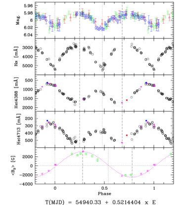
Figure 3: Phased observational data. Top panel: Photometric magnitudes from Hipparcos (green), Oksala et al. (2010, binned to 64 phase bins, blue open circles), and ASAS data (red triangles, binned to 16 phase bins) from Mikulášek et al. (2010). Second, third, and fourth panels: Equivalent width measurements of H$\alpha$, Hei$\lambda$$\lambda$ 4388, and 4713 in mÅ, in the UVES data (black circles), the 2008 FORS1 spectra (Rivinius et al. 2010, purple triangles), and the 1999 and 2004 FEROS spectra (Rivinius et al. 2008, red and blue squares, respectively). Lowermost panel: Magnetic data from FORS1 (Rivinius et al. 2010, see there a version of this plot with less data), and ESPaDOns magnetic data (open circles) in gauss and a sinusoidal fit to the FORS1 measurements. The vertical lines denote special phases discussed in the text.

3.3 Inclination and stellar mass

In terms of Bruce3 modeling, since all other relevant quantities, like period and $v\sin i$, are well constrained, the inclination effectively sets the model’s equatorial radius (since it converts $v\sin i$ to the rotation velocity) and the geometric projection onto the line of sight. As the equatorial radius is thus constrained, the modeling parameter range is chosen to include masses between 6 and 8 M_☉, considering stellar evolution: lower mass stars at the main sequence are not large enough for the required equatorial radius, neither are higher mass stars small enough. The considered range is sufficiently broad to to rely on details of the evoolution, it is, after all, just the range over which a grid is computed. The possible inferred range of effective temperature supports this mass range.

In terms of modeling, the stellar mass only scales the polar radius and the amount of gravity darkening. However, both quantities have only subtle effects on the modeled spectral lines, and results are not really conclusive. However, in one respect the model does vary strongly with these two parameters, namely in the total luminosity and in the flux seen by the observer, since they scale the size of the stellar surface through the radius and the surface temperature distribution. Therefore, the traditional approach, determining the distance with the modeled flux, can be inverted: The revised Hipparcos parallax is sufficiently precise to do so. The Hipparcos distance, $273\pm 26$ pc, is used to define a range for model fluxes; namely “near” (247 pc), “mean” (273 pc), and “far” (299 pc) distances.

We find the models for $i=80\degr$ do not have sufficient flux; they remain well under the faintest flux limit, even for the “near” distance. For $T_{\rm eff}=18\,000$ K, models for $i=70\degr$ are just in agreement with the “near” distance flux, and only models with $i=60\degr$ are compatible with the flux curve for the “mean” distance. For $T_{\rm eff}=17\,000$ K, even models with $i=60\degr$ are just compatible with the flux curve for the “near” distance. The “far” flux is too luminous to be reproduced by any of the computed parameter sets. The ultimately-adopted inclination is, therefore, $i=60\degr$ for which we assume a $\pm 10\degr$ uncertainty.

Although this still does not constrain the mass in a straightforward observational way, all the other parameters are sufficiently well-known to leave only a narrow range of physically acceptable masses. This is because we can, at least to first order, expect that the luminosity of a star of a given mass does not change with its rotational velocity.

The luminosity computed by Bruce3 modeling, however, is not constrained by the physical processes inside the stellar interior; it is just given by the temperature distribution and the stellar surface area, both of which can be chosen independently in Bruce3. The stellar evolution requirement that mass and luminosity are related is an independent constraint, taken into account only in a later step (and as well for setting a reasonable grid range above). This means the Bruce3-computed luminosity is almost invariant with model mass. Instead, it increases with decreasing inclination, in such a way that all $T_{\rm eff}=18\,000$ K, $i=60\degr$ models have a luminosity of about $L_{\star}=1120\,{\rm L_{\sun}}$, $T_{\rm eff}=17\,000$ K, $i=60\degr$ models have a luminosity of about $L_{\star}=1000\,{\rm L_{\sun}}$. Such a luminosity is only compatible with a mass of about $6\pm 0.5$ M_☉. Unfortunately, both models give a very similar distance to match the absolute flux, around 240 pc, which is only somewhat closer than the Hipparcos distance of $273\pm 26$ pc.

[Hei]$\lambda$ 4045

Hei$\lambda$ 4713

Hei$\lambda$ 6678

Nei$\lambda$ 6717

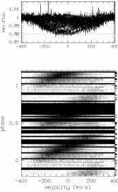
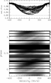
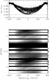
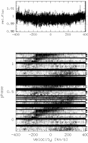
Nii$\lambda$ 4631

Cii$\lambda$ 4267

Siiii$\lambda$ 4553

Sii$\lambda$ 4816

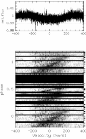
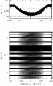
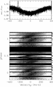
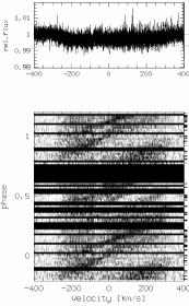
Figure 4: Phased variations of photospheric helium and metal lines, represented as dynamic spectra. Top panels: original profiles, the dotted lines mark the cuts applied for black and white in the grey-scale panels. Bottom panels: phased dynamical spectra. These panels were constructed with 32 or 64 phase bins (64: Siiii$\lambda$ 4553 and Sii$\lambda$ 4816, Hei$\lambda$ 6678, Hei$\lambda$ 4713) depending on the complexity of the variations prompting for a trade-off of higher sampling vs. the noise level. For a detailed description of the variations see Sect. 4.

So the only remaining question, left open above, is whether to adopt 17 000 or 18 000 K. While the model for 18 000K agrees better with the spectroscopic results, and has a more plausible luminosity, it would require a somewhat higher reddening than suggested by $E_{(B-V)}$. On the other hand, the model for 17 000 K provides a better fit for the spectral energy distribution, yet its luminosity would be lower by 10 to 20 % than expected even for a star of 6 M_☉ only. However, given the relatively low extinction this is a rather robust determination. For the final model, therefore, we adopt 17 500 K, but unfortunately have to accept a rather generous error margin of 1000 K.

The final parameters are summarized in Table 2, the absolute flux fit for these parameters is shown in Fig. 2. The figure illustrates that these parameters give good fits to both absolute flux and line profiles, except of course the variable helium lines, as well as some of the UV lines. Concerning the uncertainty intervals given in Table 2, we note that only the one given in the uppermost part (input parameters) were constrained traditionally, i.e. by judging a grid of model vs. observational data. The intervals given for the derived parameters, however, were obtained by propagating these input parameter uncertainties through the model code, and thus they do not necessarily satisfy the usual statistical relations (in particular, they are non-orthogonal to each other). Furthermore, since the quantities have been computed, we give more significant digits than the interval would warrant, to keep the values of the derived parameters consistent with the input parameters.

4 Photospheric abundance pattern

Figure 3 shows previously published data and equivalent widths measured in the UVES data, phased with the ephemeris given in Sect. 1.1. The uppermost panel shows the available photometric data. A constant offset on magnitude has been added to the additional data sets, taken in different photometric systems, for the purpose of display together with the Hipparcos data. We note that photometric data from different bands may not have the same amplitude, as well as shifts in phase (expressed here a linear phase $\phi$) vs. each other, but the accuracy of the available data is not sufficient to determine if this is the case here.

In any case, the data by Oksala et al. (2010) and the UVES spectra were taken only one year apart, and the period is known well enough to be sure now about the phasing of the spectroscopic variations vs. the photometric: When H$\alpha$ is in occultation, there is a photometric minimum. However, since the photometric minima are broad and the phases of occultations and Hei EW minima differ only by $\Delta\phi\approx 0.07$, the following can also be said: When the Hei absorption is weakest, there is a photometric minimum. Whether the photometric variations are due to the occultations, as suggested by Townsend (2008), or due to the photospheric abundance pattern, as suggested by Mikulášek et al. (2010), will require careful modeling, and possibly further multicolor photometric observations to distinguish geometric from intrinsic effects.

4.1 Line strength variations

The H$\alpha$ equivalent widths are fully dominated by variations of the circumstellar environment; there is no indication of an intrinsic photospheric variation of this or any other hydrogen line strength (see Fig. 7). The vertical dotted lines in the four upper panels of Fig. 3 mark the central points of the occultations, i.e. when the circumstellar lobes are centrally in front of the stellar disk (at $v_{\rm sys}$). This is at $\phi=0$, actually fixed by the definition of the ephemeris, and at $\phi=0.46$.

The third and fourth panels in Fig. 3 show the equivalent width variations of the Hei$\lambda$$\lambda$ 4713 and 4388 lines. The double wave character of the Hei equivalent width curve is very clear. Although the strongest EW points in both half-cycles are of a similar level, the weakest EW values differ by a factor of two. The dashed lines mark the estimated times of maximal He-line strength at about $\phi=0.25$ and $0.68$.

4.2 Line profile variations

The most obvious photospheric variation is that of the Hei lines. The variations are very strong, relative to the line strength much stronger than in the prototype $\sigma$ Ori E: e.g. the EW of Hei$\lambda$ 4713 varies between 250 and 550 mÅ in HR7355 vs. between 420 and 570 mÅ in $\sigma$ Ori E (measured in our own and archival data for both stars). Figure 3 shows a factor of two and four between the EWs of the weak and strong states of Hei lines. Judging the EW variations in the figure at face value, they form a simple double wave pattern that would be well compatible with just two enhanced polar regions and a depleted belt. A detailed look at the spectra, however, shows that the variations are not that easily explained.

The forbidden transition of Hei at 4045 Å (Fig. 4, upper left) shows the simplest pattern; presumably because it is the weakest line of Hei only the strongest features are seen: Two He-enhanced regions are visible, which, according to the phasing with the magnetic curve in Fig. 3, are consistent with being located at about the magnetic poles, as is typical for He-strong stars (see e.g. Groote & Hunger 1982; Reiners et al. 2000, for $\sigma$ Ori E). These two regions are also the dominant ones in other helium lines. They cross $v_{\rm sys}=v_{0}=7$ km s^-1 at $\phi_{0}=0.19$ and $\phi_{0}=0.65$.

However, the stronger lines show additional features. In Hei$\lambda$ 4713 and 6678 (Fig. 4, middle two panels in upper row) three more, albeit weak, features are seen: They cross zero velocity at $\phi_{0}=0.02$, $0.46$, and $0.88$. The position of the first two agree with the occultations (see Sect. 6). However, the time these features take to propagate across the profile (formally an inverse acceleration, in dynamical spectra directly visible as “slope” of a propagating feature), show this is not the case: The time to cross the entire range of 2 $v\sin i$ for undoubted occultation features, in all lines, is much faster, as seen at $\phi_{0}=0.46$ in the panels for Nii$\lambda$ 4631 and Siiii$\lambda$ 4553 in Fig. 4. This is so because the magnetosphere is empty (or at least far less dense) closer to the star than about 2 stellar radii, as seen by the lack of H$\alpha$ emission at velocities $<2\times v\sin i$ at quadrature, and the crossing time of a corotating feature scales inversely with the distance from the star.

In the fairly many Nei lines detected in the spectrum, like Nei$\lambda$ 6717 shown in Fig. 4 (upper right panel), there are two features crossing the profile, at $\phi_{0}=0.20$ and $\phi_{0}=0.64$. These are almost the same phases as for the strong helium features. Nei, therefore, is a metallic species that is probably enriched at the magnetic poles, rather than at the magnetic equator, as one usually observes for metals in He-strong stars.

Unfortunately, looking at more metal lines does not make the picture any simpler: While in Nii$\lambda$ 4631 only two features are seen ($\phi_{0}=0.35$ and $0.93$) four each can be identified in Cii$\lambda$ 4267 and Siiii 4553 ($\phi_{0}=0.08,0.32,0.49$, and $0.95$), and possibly as many as six are seen in Sii$\lambda$ 4816 ($\phi_{0}=0.02,0.13,0.32,0.49,0.60$, and $0.73$).

4.3 Doppler imaging

We applied the Doppler imaging (DI) technique to interpret phase-dependent behavior of some of the variable spectral lines in terms of an inhomogeneous distribution of chemical elements. Due to the strong rotational Doppler broadening of its spectra, HR 7355 is a very challenging target for DI. In fact, it has the largest $v\sin i$ among the early-type stars to which abundance DI has been applied. Due to excessive blending and shallow line profiles, only Cii$\lambda$ 4267 and strong He lines, such as Hei$\lambda$ 4713, are suitable for modeling. We used these two spectral features to derive respective abundance distributions with the updated version of the magnetic DI code described by Piskunov & Kochukhov (2002).

Since HR 7355 has a very strong magnetic field, it has to be taken into account in abundance mapping. Available Stokes $I$ observations do not allow the derivation of the magnetic field geometry simultaneously with chemical spots. We therefore adopted the 11.6 kG dipolar magnetic field model derived in the next section. On the other hand, gravity darkening and oblateness of the star were not included in the modeling. As a consequence, we might expect spurious pole-to-equator abundance gradients for the lines especially sensitive to effective temperature. For the prupose of DI, stellar parameters, i.e. inclination and $v\sin i$, were adopted as derived above form spectroscopic modeling.

The results of the DI analysis of Cii$\lambda$ 4267 are illustrated in Fig. 5. The surface distribution of carbon required to reproduce variability of this line features significant meridional gradient, possibly due to unaccounted gravity darkening. In addition, there is about 1 dex abundance contrast at high latitudes, dominated by two spots seen at rotational phases 0.25 and 0.80.

Helium is overabundant in the atmosphere of HR 7355 and shows a high-contrast surface distribution resulting in dramatic variability of Hei lines. Since concentration of He is comparable to that of H over a significant part of the stellar surface, not only is the observed line profile variability a result of the abundance dependence of the He line absorption coefficient, but is is also a consequence of continuum instensity variations and, possibly, lateral variations of the atmospheric structure. All these effects have to be accounted for in order to obtain an accurate absolute scale and magnitude of the He abundance variations. We carried out He mapping with the help of a new magnetic DI code, Invers13 (Kochukhov et al. 2012), which uses a grid of model atmospheres to treat self-consistently the impact of abundance variations on the line profiles. Our present calculations are based on the LLmodels (Shulyak et al. 2004) grid computed for $T_{\rm eff}=17500$ K, $\log g=4.0$ and the helium abundance from $\log(\mathrm{He/H})=-3.0$ to $\log(\mathrm{He/H})=1.9$.

The results of He abundance inversion are presented in Fig. 6. The overall contrast of the He map is nearly 4 dex. The main He overabundance features are located at the equator and below. To reproduce a narrow bump traveling across the He line profile at phases 0.95-0.05, the code requires a latitudinally extended spot where He is strongly underabundant relative to the Sun.

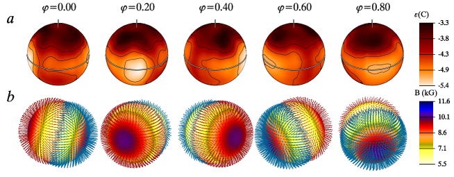
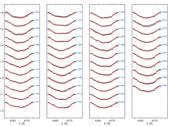
Figure 5: Carbon abundance distribution reconstructed from the variations of the Cii$\lambda$ 4267 line. The top panels show spherical maps of the abundance distribution labelled by phase with iso-abundance lines plotted with a 0.5 dex step (a) and assumed dipolar magnetic field geometry (b). The C abundance is given in the $\log(N_{\rm C}/N_{\rm tot})$ units.

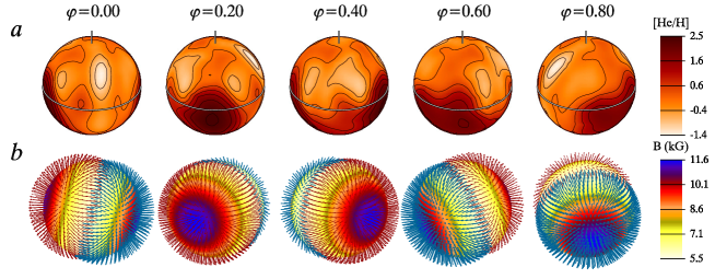
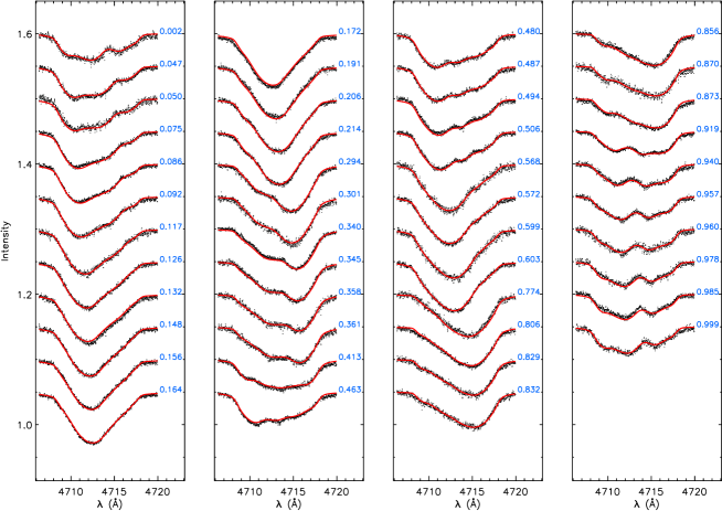
Figure 6: Same as Fig. 5 for helium distribution reconstructed using the Hei$\lambda$ 4713 line. The He abundance is given in logarithmic units relative to the Sun.

5 The magnetic field

While the high $v\sin i$ tells that the inclination cannot be small, some further constraints on both the inclination $i$ and the obliqueness of the magnetic field vs. the rotational axis $\beta$ can be obtained from the observed properties of the longitudinal magnetic field.

The magnetic field curve is not centered around zero, i.e. $B_{\rm min}\neq-B_{\rm max}$, as noted in the original papers (Oksala et al. 2010; Rivinius et al. 2010). If a dipole is assumed, this means neither $i$ nor $\beta$ can exactly be 90°, although they might be close: If the inclination was 90°, the rotational projection of the two magnetic poles must be the same, regardless of $\beta$. The same is true for $\beta=90\degr$, since then the magnetic poles would be on the rotational equator.

Although the field, for reasons discussed in Sect. 7, is most likely not exactly dipolar, the variation is sufficiently sinusoidal to apply the equations by Preston (1971) to the magnetic variation given by Rivinius et al. (2010). This yields $r=B_{\rm min}/B_{\rm max}=\cos(\beta+i)/\cos(\beta-i)=-0.78$. If the values of Oksala et al. (2010) are used, $r=-0.80$ is obtained, but this changes the values of $\beta$ and $i$ (see below) only by a few degrees. This value of $r$ means that $\beta+i$ must be smaller than or equal to 141°. If the sum is equal to 141°, then $i=\beta=70.5\degr$. If $i\neq\beta$, we can say that on the one hand, $i$ cannot be much smaller than 70° because of the large $v\sin i$, on the other hand $i$ cannot be much larger either, since then $\beta$ would have to be very small, which would make it very hard to explain the strong mean longitudinal field, unless the dipole field strength reaches several dozen kilogauss or more at the poles. We conclude that both $i$ and $\beta$ are most likely between 60 and 80°, in such a way that $\beta+i$ is about 130 to 140°. This limit to the inclination is in nice agreement with the spectroscopic determination, which is $60\pm 10\degr$.

Using Schwarzschild’s (1950) in the form given by Leone et al. (2000), and assuming a pure dipole with $i=60\degr$ and $\beta=75\degr$, the field strength at the magnetic poles would then be about 11.6 kG.

The observational indications for a non-dipole field and a non-sinusoidal field curve are subtle, so that the above values, summarized in Table 3, should at least be a good approximation.

H$\alpha$

H$\beta$

Pa₁₄

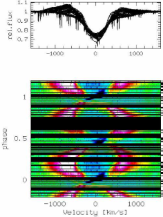
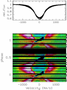
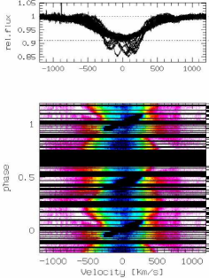
Figure 7: Observational variations of the circumstellar magnetosphere. The upper row shows the actual profiles overplotted, in the lower row the phased variations are shown. For H$\alpha$ and H$\beta$ the residuals after subtracting the Bruce3 model are used for the phased plot; the residual level in the line center is zero to better than 0.01. Emission is clearly seen in the residuals, in fact up to H$\delta$. Paschen lines show emission as well; shown here is Pa₁₄ (note the different scales of the abscissae). 128 phase bins were used for all panels in order to sample the fast variations around the occultation phases in sufficient detail.

6 The circumstellar magnetosphere

The circumstellar magnetosphere is filled with magnetically trapped gas (see e.g. Figs. 1 and 8 of Townsend et al. 2007, for an illustration of the concept and definitions). The trapped gas, according to Townsend et al., occupies a warped plane between the magnetic and rotational equator, effectively the points along each field line where the centrifugal acceleration is highest, as long as this is larger than the local gravity. However, this plane is not uniformly filled; the intersections of the magnetic and rotational equatorial planes are preferred, forming two geometrically relatively thin lobes (Townsend 2008). This gas is seen in emission in hydrogen lines when in quadrature and in absorption in hydrogen and a few other lines when passing through the line of sight. Species and lines in which the occultations are present include Hi, Oi$\lambda$ 8446 and the 777x triplet, Siii$\lambda$ 6347, Nii$\lambda$ 4631 (see respective panel in Fig. 4, at $\phi=0.46$ and $v=0$ km s^-1), and many Feii lines (Feii$\lambda$ 4949 is visible in the Siiii$\lambda$ 4553 panel in Fig. 4, at $\phi=0.46$ and $v=-200$ km s^-1).

Table 3: Magnetic parameters. The inclination $i=60\pm 10\degr$ is taken from Table 2

.

Field parameters
$\beta$	$75\pm 10\degr$
Polar $B_{\rm dipole}$	11.6 kG
Magnetospheric lobe parameters
Inner radius	2 R⋆
Outer radius	4 R⋆
Particle density	$10^{12.3\pm 0.5}{\rm cm}^{-3}$
Plane tilt	$<22\degr/\cos i$
Lobe separation	$165\pm 5\degr$

6.1 Geometry

The two occultations occur at phases $\phi=0.0$ and $\phi=0.46$ (Fig. 7). The phenomena associated with the passing of the magnetospheric lobes in front of the star provide information on the circumstellar geometry. The lobe absorption is a relatively narrow feature, of a FWHM of only about 250 km s^-1 in Pa₁₄. This value is similar in other lines. This corresponds to about 40 % of $2\times(v\sin i)$. Since the circumstellar gas is locked to the magnetosphere, it is in co-rotation with the stellar surface. For this reason any projected radial velocity interval is unambiguously mapped onto a strip parallel to the projected rotational axis, and the width of such an interval translates directly to geometry: A $90\degr$ tilt would produce zero width (as only one velocity would be obscured at any given time), while a $0\degr$ tilt would obscure all velocities across $2\times(v\sin i)$ simultaneously. Hence, the projection of the tilt of the plane of the lobes against the rotational axis must then be around the arcus tangens of the simultaneous velocity dispersion of the circumstellar absorption in units of $2\times(v\sin i)$, which in this case is $\arctan 0.4=22\degr$. This actually is an upper limit, if a non-zero scale height for the lobes was assumed, the inclination had to be even lower. Note, however, that this tilt is not just a projection of $90\degr-\beta$, since the plane of the lobes is somewhat warped. Nevertheless, it is probably close to this value.

An equatorial feature in bound corotation, traversing the line of sight at photospheric level, would take half a cycle to do so ($\Delta\phi=0.5$). With increasing distance, the crossing time, i.e. the fraction of the orbit within a line of sight impact parameter $<1$, decreases quadratically. The passing of the lobe through the line of sight towards the star is much faster than $\Delta\phi=0.5$: from $-v\sin i$ to $+v\sin i$ takes the feature about $\Delta\phi=0.13$. i.e. about one fourth of the crossing time as in case material would be present down to the stellar surface. ThereforeCombining this and the quadratic decrease with distance, it can be concluded that there is no absorbing material directly above the star, but sufficient density to absorb is found only at and above a radius of $2\,R_{\star}$.

Outside the occultation phases, the emitting material is seen next to the stellar disk, and again since it is in magnetically bound corotation there is a linear relation between rotational velocity and distance from the stellar surface, meaning material at twice the radius has twice the rotational velocity. Thus, when the circumstellar material is in quadrature, the observed velocities give additional geometry information: The emission has an inner edge at about $600$ km s^-1, which again points to an empty region inside 2 R_⋆. The outer edge of the emission is at a velocity of about $4\times v\sin i$ in H$\alpha$ and $3\times v\sin i$ in Pa₁₄, which gives outer limits for the lobe emission of about 4 R_⋆ and 3 R_⋆, respectively.

There is also a “skew” in the appearance of the emitting lobes, well seen in Fig. 7. Tracing the maximum emission levels belonging to each lobe, it is found that each lobe varies in a sinusoidal shape, i.e. the cardinal points of conjunctions and quadratures are separated by a quarter of a cycle, but the two lobes are separated by less than half a cycle, i.e. geometrically by less than 180°. That difference is the same as the one that causes the second occultation to be at $\phi=0.46$ instead of at $\phi=0.5$.

Table 4: Equivalent width of the circumstellar emission in the Balmer lines and the computed Balmer decrements for two phases and the red and blue emission peaks separately.

	Equivalent widths [Å]			Balmer decr.
	H$\alpha$	H$\beta$	H$\gamma$	$D_{34}$	$D_{54}$
Blue, $\phi=0.17$	$-1.37$	$-0.42$	$-0.17$	1.16	0.59
Red, $\phi=0.17$	$-0.94$	$-0.25$	$-0.13$	1.33	0.76
Blue, $\phi=0.78$	$-1.00$	$-0.33$	$-0.14$	1.07	0.62
Red, $\phi=0.78$	$-1.17$	$-0.26$	$-0.08$	1.59	0.45

6.2 Density

The theoretical line profiles are a very good approximation of the mean photospheric profiles, as seen in Fig. 2 for H$\gamma$ and Fig. 7 for H$\beta$ and H$\alpha$. Therefore, the residuals faithfully represent the pure circumstellar emission and it is possible to apply nebular diagnostics and calculate Balmer decrements. The Balmer decrements $D_{34}$ and $D_{54}$ were measured separately for the blue- and redshifted emission peaks at phases 0.17 and 0.78, when the emitting material is seen next to the star (see Table 4). For computing the decrements, the same method as used by Štefl et al. (2003) for the classical Be star 28 CMa was adopted. The stellar continuum fluxes to correct for the normalization were those modeled by Bruce3, so that $f_{\star}({\rm H}\alpha)/f_{\star}({\rm H}\beta)=0.35$ and $f_{\star}({\rm H}\gamma)/f_{\star}({\rm H}\beta)=1.46$. The measured values were compared to the theoretical computations by Williams & Shipman (1988), which were derived for an isothermal pure hydrogen accretion disk of 10 000 K, that is optically thin in the continuum. The Balmer decrements depend only weakly on temperature in such a hot plasma, so that even if the circumstellar material of HR 7355 is hotter than 10 000 K the derived densities still provide useful guidelines for modeling. While the values for $D_{54}$ would be in agreement with logarithmic particle densities between 11.7 and 12.5 per cm³, the logarithmic particle densities inferred from $D_{34}$ are somewhat higher, at 12.2 to 12.8 per cm³. In any case, these values are close to the optically thick limit, above which the decrements become independent of density.

7 Discussion

7.1 HR 7355 as a rapid rotator

HR 7355 was the first magnetic star discovered to rotate so rapidly that rotational effects like oblateness and gravity darkening should be taken into account. A second example, HR 5907, has been published by (Grunhut et al. 2012). Due to the relative proximity of HR 7355 not only was it possible to obtain high quality data, but the public archives contain data for the star as well.

Using all these data, the five parameters required to describe a rapidly rotating star could be derived (Table 2). Of these five, two stand out: Firstly, the effective temperature of just 17 500 K. This is fairly low for a spectral classification of B2. We note, however, that B2 is the spectral subtype at which Hei lines are strongest, and so the classification for a star with helium overabundance will be biased towards that spectral subtype with respect to its temperature. Although the Doppler imaging indicates that not the entire surface is overabundant in helium; with patches of both over- and underabundance existing, the stellar surface on average is overabundant in helium, justifying its classification as He-strong in earlier papers (Oksala et al. 2010; Rivinius et al. 2010).

The second unusual parameter is the rotation rate, at almost 90% of the critical value (even the previous record holder for rapid rotation among non-degenerate magnetic OB stars, $\sigma$ Ori E barely reached 50%). This means that no significant rotational spin-down can have occurred for HR 7355 yet. Unless the field is self-generated and has only existed since recent times, this leaves two possibilities: Either the star is so young that it had no time to brake yet, or the mass loss is so weak that it does not remove any significant amount of angular momentum. While the latter would have been unlikely for a star of 22 000 K, i.e. corresponding to a normal B2 star, it is much more plausible for a star of only 17 500 K. For the very similar HR 5907, Grunhut et al. (2012) obtain a spin-down timescale of 8 Myr. This is still less than the 15 to 25 Myr suggested by Mikulášek et al. (2010). However, for an age of less than 8 Myr our stellar parameters, i.e. gravity, mass, polar radius, and luminosity, agree with evolutionary models. Even at a distance of only 236 pc the conclusion by Mikulášek et al. (2010), namely that HR 7355 is probably not a member of Scorpius-Centaurus, stands.

7.2 Magnetic field geometry

While for a photospheric parameter analysis the tools exist to take rotation into account, such tools for the magnetic analysis are only being developed and have not yet reached the parameter space required here, simply because the inclusion of such strong effects was not necessary to date. The most rapid rotation taken into account for magnetic analysis so far was by Khalack (2005), limited to $R_{\mathrm{pole}}/R_{\mathrm{eq}}<0.95$. In the following discussion, the effects of the rapid rotation are speculated about, but we stress firm conclusions will require more sophisticated theoretical work to be done.

A sinusoidal variation of the longitudinal magnetic field is the hallmark of a centered dipole field tilted with respect to the rotation axis. However, the high-quality spectroscopic data suggest that the field topology may be more complex than this. With the circumstellar clouds situated at the intersections between magnetic and rotational equators, the cloud transits should be coincident with $B_{z}=0$. The measured magnetic curve, when fitted with a sine, has an offset of $+0.3$ kG. The magnetic nulls are expected to occur at $\phi=0$ and $\phi=0.54$ (dotted lines in lowermost panel of Fig. 3). However, the cloud transits are observed to occur at $\phi=0.0$ and $\phi=0.46$ (dotted lines in upper panels of Fig. 3). The maximal strength of the Hei lines normally coincides with the magnetic poles pointing towards the observer. This would be expected for $\phi=0.28$ and $0.78$ in case of a sinusoidal variation (dashed lines in lowermost panel of Fig. 3), but spectroscopically, i.e. estimated by maximal He-enhancement, occurs at $\phi=0.25$ and $0.68$ (dashed lines in upper panels of Fig. 3).

Offsets as discussed in the previous poaragraph could theoretically be explained in case of a de-centered magnetic dipole. The two misaligned cloud crossings would require an offset of the dipole along the magnetic polar axis. Such an offset could also account for the constant term of 0.3 kG in the field curve, although this alone could also be explained by the projection topology of an aligned field. The observed timing of the magnetic poles facing towards the observer requires an offset perpendicular to this axis. These offsets would show in a non-sinusoidal variability curve of the magnetic field. In any case, however, off-center dipoles, or any combination of low order multipole components, can only be a simplified approximation to the actual magnetic field, as magnetic Doppler imaging has shown that more complex and small scale structures are usually present even for stars with largerly sinusoidal variations in the longitudinal field (Kochukhov et al. 2011).

The line profile variations are surprisingly complex, with at least four, possibly as many as six subfeatures identifiable in some lines. It is surprising that a relatively strong and ordered field as in HR 7355 gives rise to so many clearly distinct zones of helium and metal abundances. One possibility to be explored could be an interplay of a more simple type of abundance variation pattern with the co-latitude dependent line formation in a rapidly rotating star due to the gravity darkening.

7.3 The magnetosphere

The circumstellar magnetosphere is filled with dense gas, sufficiently dense to make the Balmer emission optically thick. Since the gas needs to be ionized to be trapped by the magnetic field, one might wonder whether in the central regions of this dense gas this is still the case. The occultation pattern observed in other line transitions can be used for guidance to answer this question: The signature of the occultation of the central, most dense part of the magnetosphere is seen in lines of Feii, Nii, Siii etc. It is not seen, however, in the lower excitation/ionization lines of Caii or Nai. This means that the temperature of the magnetosphere is still of the order of 10 000 K, where hydrogen is still far more than sufficiently ionized to be locked to the magnetic field.

7.4 Comparison to $\mathbf{\sigma}$ Ori E and HR 5907

The prototype of an emission line magnetosphere star is ${\sigma}$ Ori E. It is, in fact, fairly similar to HR 7355: It is He-strong, with similar polar field strength and $i=75\degr$ and $\beta=55\degr$. The two main differences concerning parameters are the higher effective temperature (23 000 K) and slower rotation (less than 50% critical) of ${\sigma}$ Ori E (see e.g. Oksala et al. 2012, for the most recent parameter determination). As a consequence of geometry and field strength, the circumstellar variations are comparable, except for the lower $v\sin i$. Fig. 5 of Oksala et al. is extremely similar to our Fig. 7. As well, occultation crossings can be seen in metal ions of ${\sigma}$ Ori E, as in Fig. 6 of that work, Feiii$\lambda$ 5127 at $\phi=0$, vs. our Fig. 4, Nii$\lambda$ 4631 at $\phi=0.46$. A morphological difference, for which it is not clear how it is associated with the parameters, is that the equivalent width changes due to the surface chemical abundance pattern are of much lower amplitude in ${\sigma}$ Ori E than in HR 7355.

Shortly after HR 7355 was confirmed to be a magnetic star (Oksala et al. 2010; Rivinius et al. 2010), a very similar object with an even shorter period was found, HR 5907 (Grunhut et al. 2011, 2012). Mass, effective temperature, and inclination of HR 7355 and HR 5907 are within each other’s error bars (see Table 2), and the period as well hardly differs with 0.521 d vs. 0.508 d. The equatorial velocity of HR 5907 is somewhat slower, and the equatorial radius smaller than for HR 7355, so that HR 5907 is less luminous, but the average photospheric spectra of HR 7355 and HR 5907 are virtually identical. Also the dipolar field strength for both is of the order of 10 kG, and the gas density of the magnetosphere is comparable as well.

The only strong difference is the obliquity of the field, being much smaller for HR 5907 (almost aligned, $\beta=7\degr$), which, however, has striking effects on the variability. The amplitude of the line profile variability is much smaller in HR 5907, since the magnetic equatorial belt is visible to the observer all the time, and the contributions from the pole only vary slightly, while for HR 7355 magnetic pole-on and equator-on views alternate. Nevertheless the actual profile variability is still much more complex than in slower rotators, even if the equivalent width amplitude is very small. As pointed out by Townsend (2008), the low obliquity also leads to only one occultation per rotational cycle, while HR 7355 has two. As well due to this the emission variability of HR 5907 is not a clear double-helix pattern as for HR 7355.

8 Conclusions

We have shown that HR 7355 is an early B type magnetosphere star. In principle similar to the well known $\sigma$ Ori E, it stands out as the non-degenerate magnetic star rotating most closely to the critical limit, at about 90%, followed by HR 5907. The magnetic field of HR 7355 has a polar strength of about 11 to 12 kG, with a morphology close to, but as suggested by the asymmetries in the equivalent width curves probably not exactly dipolar, and with a fairly large obliquity of $75\degr$, seen at an inclination of about $60\degr$.

The stellar parameters point to a relatively young star with an effective temperature typical for a mid B rather than an early B type star, namely 17 500 K. As the typical mass-loss rate for such a temperature is significantly less than for a B2 type star, the spin-down timescale is several Myr, and hence the age and rapid rotation are not inconsistent with the presence of a fossil magnetic field.

The stellar surface shows strong abundance variations, which have been Doppler imaged for helium and carbon in this work. Although some small surface areas in the Doppler imaging have a helium abundance lower than the solar value, helium enriched areas dominate. Indeed, compared to a model with typical solar or B-star abundances, the Hei lines are stronger in the time averaged profile. This is also the explanation for the spectral classification as type B2 in spite of the effective temperature of only 17 500 K.

As recently as ten years ago, $\sigma$ Ori E was the only B-type magnetic star with an emission line magnetosphere, and $\theta^{1}$ Ori C was the only such O star. In the last few years this situation has changed, and HR 7355 is not only a new member of the growing class of magnetosphere emission line stars, but has doubled the parameter space for these objects in the rotational dimension. Density estimates for the magnetospheric region are similar in all three B stars mentioned ($\sigma$ Ori E, HR 5907, HR 7355).

References

- Boggess et al. (1978) Boggess A., Carr F. A., Evans D. C., Fischel D., Freeman H. R., Fuechsel C. F., Klinglesmith D. A., Krueger V. L., Longanecker G. W., Moore J. V., 1978, Nature, 275, 372
- Cardelli et al. (1989) Cardelli J. A., Clayton G. C., Mathis J. S., 1989, ApJ, 345, 245
- Collins (1963) Collins II G. W., 1963, Astrophysics, 138, 1134
- Dekker et al. (2000) Dekker H., D’Odorico S., Kaufer A., Delabre B., Kotzlowski H., 2000, in M. Iye & A. F. Moorwood ed., Society of Photo-Optical Instrumentation Engineers (SPIE) Conference Series 4008 p. 534
- Gray (1998) Gray R. O., 1998, AJ, 116, 482
- Grønbech & Olsen (1976) Grønbech B., Olsen E. H., 1976, A&AS, 25, 213
- Groote & Hunger (1982) Groote D., Hunger K., 1982, A&A, 116, 64
- Grunhut et al. (2012) Grunhut J. H., Rivinius T., Wade G. A., Townsend R. H. D., Marcolino W. L. F., Bohlender D. A., Szeifert T., Petit V., Matthews J. M., Rowe J. F., Moffat A. F. J., Kallinger T., Kuschnig R., Guenther D. B., Rucinski S. M., Sasselov D., Weiss W. W., 2012, MNRAS, 419, 1610
- Grunhut et al. (2011) Grunhut J. H., Wade G. A., Rivinius T., Marcolino W. L. F., Townsend R. H. D., Townsend 2011, in C. Neiner, G. Wade, G. Meynet, & G. Peters ed., IAU Symposium 272 Discovery of the most rapidly-rotating, non-degenerate, magnetic massive star by the MiMeS collaboration. pp 190–191
- Hubeny & Lanz (2011) Hubeny I., Lanz T., 2011, in Astrophysics Source Code Library, record ascl:1109.022 Synspec: General Spectrum Synthesis Program. p. 9022
- Khalack (2005) Khalack V. R., 2005, A&A, 429, 677
- Kochukhov et al. (2005) Kochukhov O., Khan S., Shulyak D., 2005, A&A, 433, 671
- Kochukhov et al. (2011) Kochukhov O., Rivinius T., Oksala M. E., Romanyuk I., 2011, in C. Neiner, G. Wade, G. Meynet, & G. Peters ed., IAU Symposium 272 pp 166–171
- Kochukhov et al. (2012) Kochukhov O., Wade G. A., Shulyak D., 2012, ArXiv e-prints
- Kurucz (1992) Kurucz R. L., 1992, in B. Barbuy & A. Renzini ed., IAU Symposium 149 Model Atmospheres for Population Synthesis. p. 225
- Lanz & Hubeny (2007) Lanz T., Hubeny I., 2007, ApJS, 169, 83
- Leone et al. (2000) Leone F., Catanzaro G., Catalano S., 2000, A&A, 355, 315
- Mikulášek et al. (2010) Mikulášek Z., Krtička J., Henry G. W., de Villiers S. N., Paunzen E., Zejda M., 2010, A&A, 511, L7
- Oksala et al. (2010) Oksala M. E., Wade G. A., Marcolino W. L. F., Grunhut J., Bohlender D., Manset N., Townsend R. H. D., Mimes Collaboration 2010, MNRAS, 405, L51
- Oksala et al. (2012) Oksala M. E., Wade G. A., Townsend R. H. D., Owocki S. P., Kochukhov O., Neiner C., Alecian E., Grunhut J., 2012, MNRAS, 419, 959
- Papaj & Krelowski (1992) Papaj J., Krelowski J., 1992, Acta Astronomica, 42, 211
- Piskunov & Kochukhov (2002) Piskunov N., Kochukhov O., 2002, A&A, 381, 736
- Preston (1971) Preston G. W., 1971, PASP, 83, 571
- Reiners et al. (2000) Reiners A., Stahl O., Wolf B., Kaufer A., Rivinius T., 2000, A&A, 363, 585
- Rivinius et al. (2010) Rivinius T., Szeifert T., Barrera L., Townsend R. H. D., Štefl S., Baade D., 2010, MNRAS, 405, L46
- Rivinius et al. (2008) Rivinius T., Štefl S., Townsend R. H. D., Baade D., 2008, A&A, 482, 255
- Schwarzschild (1950) Schwarzschild M., 1950, ApJ, 112, 222
- Shulyak et al. (2004) Shulyak D., Tsymbal V., Ryabchikova T., Stütz C., Weiss W. W., 2004, A&A, 428, 993
- Townsend (1997) Townsend R. H. D., 1997, MNRAS, 284, 839
- Townsend (2008) Townsend R. H. D., 2008, MNRAS, 389, 559
- Townsend et al. (2007) Townsend R. H. D., Owocki S. P., Ud-Doula A., 2007, MNRAS, 382, 139
- Štefl et al. (2003) Štefl S., Baade D., Rivinius T., Otero S., Stahl O., Budovičová A., Kaufer A., Maintz M., 2003, A&A, 402, 253
- Williams & Shipman (1988) Williams G. A., Shipman H. L., 1988, ApJ, 326, 738
- Zahn (2011) Zahn J.-P., 2011, in C. Neiner, G. Wade, G. Meynet, & G. Peters ed., IAU Symposium 272 pp 14–25