Choice of boundary condition for lattice-Boltzmann simulation of moderate Reynolds number flow in complex domains

Abstract

Modeling blood flow in larger vessels using lattice-Boltzmann methods comes with a challenging set of constraints: a complex geometry with walls and inlet/outlets at arbitrary orientations with respect to the lattice, intermediate Reynolds number, and unsteady flow. Simple bounce-back is one of the most commonly used, simplest, and most computationally efficient boundary conditions, but many others have been proposed. We implement three other methods applicable to complex geometries (Guo, Zheng and Shi, Phys Fluids (2002); Bouzdi, Firdaouss and Lallemand, Phys. Fluids (2001); Junk and Yang Phys. Rev. E (2005)) in our open-source application HemeLB. We use these to simulate Poiseuille and Womersley flows in a cylindrical pipe with an arbitrary orientation at physiologically relevant Reynolds (1–300) and Womersley (4–12) numbers and steady flow in a curved pipe at relevant Dean number (100–200) and compare the accuracy to analytical solutions. We find that both the Bouzidi-Firdaouss-Lallemand and Guo-Zheng-Shi methods give second-order convergence in space while simple bounce-back degrades to first order. The BFL method appears to perform better than GZS in unsteady flows and is significantly less computationally expensive. The Junk-Yang method shows poor stability at larger Reynolds number and so cannot be recommended here. The choice of collision operator (lattice Bhatnagar-Gross-Krook vs. multiple relaxation time) and velocity set (D3Q15 vs. D3Q19 vs. D3Q27) does not significantly affect the accuracy in the problems studied.

I Introduction

In the last two decades, lattice-Boltzmann methods (LBM) Succi (2001); Chen and Doolen (1998); Aidun and Clausen (2010) have been widely studied and used for fluid flow problems. We are particularly interested in its application to the study of hemodynamics: the flow behavior of blood under physiological conditions. Accurate simulation of the flow of blood in an individual could have near-term clinical benefits for, inter alia, the treatment of aneurysms Kung et al. (2011); Villa-Uriol et al. (2010); He et al. (2008) or stenoses Spilker et al. (2007); Taylor and Figueroa (2009); Tahir et al. (2011).

Applications such as these have a number of challenges (retaining computational performance in a relatively sparse, three-dimensional (3D) fluid domain; capturing the complex rheology of a dense suspension of deformable particles; accounting for the compliance of vessel walls) but here we address the choice of boundary condition method in complex domains. We will not examine the rheology and compliance problems in this article, restricting ourselves to a Newtonian fluid within a rigid-walled system, but instead aim to provide recommendations for the choice of boundary condition method(s) for a complex geometry. This choice is examined in the context of two other variables: the discrete velocity set and lattice-Boltzmann collision operator. Bearing in mind recent controversy over the reproducibility of computational science Merali (2010); Morin et al. (2012), we have released the source code of our application HemeLB for the community’s scrutiny and use.

Lätt et al. Lätt et al. (2008) considered five boundary conditions and assessed their accuracy. However, they studied only boundary conditions in which the wall passes through a lattice point, immediately restricting their results to boundaries that are normal to one of the Cartesian directions of the underlying grid. Boyd et al. Boyd et al. (2004) compared simple bounce-back to the Guo-Zheng-Shi method Guo et al. (2002) in simulations of arterial bifurcations, finding that the two methods give different results when stenosis is present, but without any analysis suggesting which, if either, is more accurate. Stahl et al. Stahl et al. (2010) performed LBM simulations with simple bounce-back boundary conditions to examine the effect of staircased boundaries (where walls that are not aligned with the underlying grid are approximated by a set of grid edges) on the measurements of shear stress both at the wall and in the bulk flow, finding errors in the shear stress of up to 35% for two-dimensional (2D) channel flow and 28% for 2D bent-pipe flow. They also introduced a method for estimating the local wall normal from the shear stress tensor. Pan et al. Pan et al. (2006) have studied the effect of different boundary conditions in porous media for flows at low Reynolds number, concluding that interpolation at the boundaries significantly improves accuracy.

In this paper we comprehensively compare the accuracy of simulations performed with some of the most widely used solid-fluid boundary conditions against analytical solutions relevant for simulations of blood flow in the larger vessels. The outline of the paper is as follows. In Sec. II we briefly introduce the lattice-Boltzmann method and discuss the collision operators, velocity sets and boundary conditions used. Our open-source software hem and simulation protocols are described, and results given in Sec. III. We present our conclusions in Sec. IV.

II The lattice-Boltzmann method

Here we provide a brief summary of the lattice-Boltzmann method (LBM); for a full derivation, we refer the reader to one of the many thorough descriptions available Chen and Doolen (1998); Succi (2001); Aidun and Clausen (2010). LBM operates at a mesoscopic level, storing a discrete-velocity approximation to the one-particle distribution functions of the Boltzmann equation of kinetic theory Liboff (1998), $\{f_{i}(\mathbf{r},t)\}$, on a regular lattice, with grid spacing $\Delta x$. The set of velocities $\{\mathbf{c}_{i}\}$ is chosen such that the distances travelled in one timestep ($\Delta t$), $\mathbf{e}_{i}=\mathbf{c}_{i}\Delta t$, are lattice vectors and to ensure Galilean invariance Qian et al. (1992). When one only wishes to reproduce Navier-Stokes dynamics, the set is typically a subset of the Moore neighborhood, including the rest vector. For 3D simulations, the most commonly used sets have 15, 19 and 27 members (termed D3Q15, D3Q19 and D3Q27, respectively). The LBM can be shown, through a Chapman-Enskog expansion, to reproduce the Navier-Stokes equations in the quasi-incompressible limit with errors proportional to the Mach number squared.

In the absence of forces, the density $\rho(\mathbf{r},t)$ and the velocity $\mathbf{u}(\mathbf{r},t)$ at a fluid site can be calculated from the distributions by

$$\rho = \sum_{i}f_{i},$$ (1)

$$\rho\mathbf{u} = \sum_{i}f_{i}\mathbf{c}_{i}.$$ (2)

Advancing the system one timestep is conceptually divided into two stages. The first is collision, which relaxes the distributions towards a local equilibrium (we denote the post-collisional distributions as $f_{i}^{\star}$):

$$f_{i}^{\star}(\mathbf{r},t)=f_{i}(\mathbf{r},t)+\hat{\Omega}(f_{i}(\mathbf{r},t)),$$ (3)

where $\hat{\Omega}$ is a the collision operator. The second is streaming, where the post-collisional distributions are propagated along the lattice vectors to new locations in the lattice, defining the distributions of the next timestep:

$$f_{i}(\mathbf{r}+\mathbf{c}_{i}\Delta t,t+\Delta t)=f_{i}^{\star}(\mathbf{r},t).$$ (4)

II.1 Collision operators

The collision operator approximates the microscopic interparticle interactions. Here we summarize the two considered in this article: lattice Bhatnagar-Gross-Krook and multiple relaxation time.

Lattice Bhatnagar-Gross-Krook (LBGK) Qian et al. (1992); Chen et al. (1992) approximates the collision process as relaxation towards a local equilibrium (see below), in a discrete velocity analogue of the Boltzmann-BGK approximation from kinetic theory Bhatnagar et al. (1954),

$$\hat{\Omega}(f_{i})=-\frac{(f_{i}-f^{\textrm{eq}}_{i})}{\tau}\Delta t,$$ (5)

where $\tau$ is the relaxation time. In this case all modes relax towards equilibrium at the same rate. This can be shown, through a Chapman-Enskog expansion (see, e.g., Ladd and Verberg (2001); Chen and Doolen (1998)), to reproduce the Navier-Stokes equations with a kinematic viscosity $\nu$ given by

$$\nu=c_{\textrm{s}}^{2}(\tau-\Delta t/2).$$ (6)

For the equilibrium distribution, we use a second-order (in velocity space) approximation to a Maxwellian distribution

$$f^{\textrm{eq}}_{i}(\rho,\mathbf{u})=\rho w_{i}\left(1+\frac{\mathbf{c}_{i}\cdot\mathbf{u}}{c_{\textrm{s}}^{2}}+\frac{(\mathbf{c}_{i}\cdot\mathbf{u})^{2}}{2c_{\textrm{s}}^{4}}-\frac{\mathbf{u}\cdot\mathbf{u}}{2c_{\textrm{s}}^{2}}\right),$$ (7)

where the weights $w_{i}$ and speed of sound $c_{\textrm{s}}$ depend on the choice of velocity set. LBGK is simple to implement and gives excellent performance; it is therefore widely used.

Multiple relaxation time (MRT) collision operators, developed at the same time as LBGK d’Humières (1992), generalize the notion of relaxation towards local equilibrium (the same as above) by allowing different relaxation rates for different moments of the distributions, potentially improving stability properties and accuracy d’Humières et al. (2002). The eigenvalue of the collision matrix which corresponds to the relaxation of shear stress $\lambda_{\textrm{shear}}$ determines the viscosity as in (6) ($\tau\rightarrow 1/\lambda_{\textrm{shear}}$). We use the MRT operator on the D3Q15 and D3Q19 lattices, as described by d’Humières et al. d’Humières et al. (2002). Here, the distribution function $f_{i}$ are transformed into the moment basis $m_{i}$ by the matrix $M_{ij}$ and the different moments can be relaxed towards equilibrium at different rates, before being projected back into the distribution space for advection

$$\hat{\Omega}(f_{i})=-\sum_{j}M^{-1}_{ij}s_{j}(m_{j}-m^{\textrm{eq}}_{j}),$$ (8)

where $s_{j}$ is the relaxation rate for mode $j$.

II.2 No-slip boundary conditions

Boundary conditions for LBM have some additional complications compared to boundary conditions for Navier-Stokes based methods, due to the LBM’s mesoscopic nature. Typically, one wishes to impose conditions on the macroscopic, hydrodynamic variables ($p$, $\mathbf{u}$) but these must be implemented through a closure relation for the mesoscopic distributions. There is no single, obviously superior choice. In this section, we will briefly review some commonly used boundary condition methods for lattice-Boltzmann models which impose the no-slip condition that the velocity of fluid adjacent to a wall is equal to the velocity of the wall.

Many boundary condition methods do not vary their behavior with respect to the location of the walls in relation to the Eulerian grid. The wall is often assumed to pass infinitesimally close to a point, the grid point remaining inside the fluid domain (sometimes referred to as “wet node” boundary conditions Lätt et al. (2008)), or alternatively the boundary is considered to be halfway along the lattice vector to a point outside the fluid. In the case of complex or non-lattice-aligned domains, these methods (and simple bounce-back, see below) will always cause a first-order modeling error, irrespective of the order of numerical accuracy of the resulting lattice-Boltzmann method. (Typically second order accuracy is sought, since this is the inherent accuracy of standard lattice-Boltzmann methods in bulk fluids.) This point has been studied numerically by Stahl et al. Stahl et al. (2010). Other boundary conditions allow the wall to be at an arbitrary position along the link between a solid and a fluid site. These reduce the modeling error of fixed wall position methods, but often at the price of increased complexity and/or the requirement of data from neighboring fluid lattice points. Further, a number of methods suffer reduced accuracy at sites in corners, which can reduce the accuracy of simulations throughout the domain.

There are a number of popular methods Inamuro et al. (1995); Zou and He (1997); Lätt (2007); Ansumali and Karlin (2002) that can only operate on straight, axis-aligned planes and force the boundary to pass directly through the lattice point. Malaspinas et al. Malaspinas et al. (2011) generalized the regularized method Lätt (2007) to cope accurately with corner nodes. The authors acknowledge that it fails for the case of a D3Q15 lattice and a right-angled corner and this method also forces the boundary to pass through a lattice point. These methods are, therefore, unsuitable for problems involving complex boundaries.

Simple bounce-back (SBB) is perhaps the most widely used boundary condition for solid walls, positioning them halfway along the lattice vector from fluid to solid. It is straightforward to implement and gives second-order accurate simulation results for flat boundaries aligned with the Cartesian axes of the lattice Ziegler (1993), although in more complex cases this degrades to first-order accuracy Ginzbourg and Adler (1994). It is also computationally cheap and local in its operation. SBB ensures conservation of mass up to machine precision. In this work we use the halfway bounce-back scheme Ladd (1994). Despite SBB exhibiting the modeling error mentioned above, we include it in this study due to its wide use.

The Bouzidi-Firdaouss-Lallemand (BFL) method Bouzidi et al. (2001) starts with simple bounce-back, but interpolates the value of the to-be-propagated distribution with the distribution at the fluid site which standard bounce-back would stream it to. They present two variants: one using linear interpolation and another using quadratic interpolation. In the present work, we restrict our attention to the linear case, due to its locality and smaller communication requirement (indeed, it can be implemented without any inter-process communication above the normal lattice-Boltzmann streaming step, albeit at a price of revisiting the sites adjacent to the wall). Bouzidi et al. claim that both variants show second-order convergence, but with the linear method having a poorer prefactor Bouzidi et al. (2001). The method as presented by Bouzidi et al. may, depending upon the distance of the wall from the fluid site, fail when computing $f_{i}(\mathbf{x},t+\Delta t)$ where $\mathbf{x}-\mathbf{e}_{i}$ lies outside the fluid domain, if the site at $\mathbf{x}+\mathbf{e}_{i}$ is also outside. Since this can occur in a curved domain, in these cases we fall back to performing SBB. While this does degrade accuracy slightly, it does appear to offer good stability of the simulation.

Guo, Zheng, and Shi (GZS) Guo et al. (2002) present a boundary condition which decomposes the unknown distributions at the wall into equilibrium and non-equilibrium parts. The equilibrium part uses the density of the fluid site and a linearly extrapolated velocity such that the velocity at the solid wall is as imposed. For the non-equilibrium part, the value from the fluid site (or the next site into the bulk) is used. The method as described in Guo et al. (2002) has the same problem as BFL. We again fall back to SBB when this occurs.

Junk and Yang (JY) Junk and Yang (2005a) propose a correction to the simple bounce-back method. They claim an advantage compared to interpolation-based methods such as GZS and BFL as their method is completely local and is able to handle non-straight boundaries where sites have lattice vectors in opposite directions, both crossing the solid-fluid boundary. The method arises from their analysis Junk and Yang (2005b) of boundary conditions for LBM in terms of general methods for studying finite difference schemes rather than the standard Chapman-Enskog expansion. By adding correction terms to the collision operator and then discretizing them in an optimal (under their analysis framework) manner, they ensure the Navier-Stokes equations are obeyed with the correct boundary conditions.

The multireflection method by Ginzburg and d’Humières Ginzburg and d’Humières (2003) uses linear combination of five neighboring distribution functions along a link direction plus a correction to determine the unknowm direction. This combination is obtained from a Chapman-Enskog expansion at the boundary sites, which is third-order accurate for steady flows. Chun and Ladd Chun and Ladd (2007) present a method based only on interpolation of the equilibrium part of the distribution functions, relying on the fact that the non-equilibrium part is always one order higher in the Chapman-Enskog expansion. Chun and Ladd demonstrate numerically that their method is advantageous for problems with many small gaps, such as porous media.

It is well known that LBGK combined with SBB does not locate the plane of zero velocity exactly halfway along the link for flows with varying velocity gradients He et al. (1997) and that this can be a significant issue in, for example, porous media Pan et al. (2006). The effective width of the channel in lattice units $H$, for a Poiseuille flow in a 2D lattice-aligned channel, driven by a constant body force is given by (Eq. (19) from Luo et al. (2011))

$$H^{2}=N_{x}^{2}+48\nu^{4}-1$$ (9)

where $N_{x}$ is the number of lattice points across the channel and $\nu$ is the viscosity in lattice units. While this error can be reduced by optimizing the choice of MRT relaxation times d’Humières and Ginzburg (2009), it can only reach zero for particularly simple cases. Typically at $\mathrm{Re}\geq 1$ the larger system sizes and smaller relaxation times combine to reduce the relative error. For example with $N_{x}=40$ and $\tau=0.55$ the effective width is 39.987, a relative error of $0.03\%$. Due to the smallness of these errors in the problems studied here, we do not consider them further.

We also note that some authors propose the use of grid-refinement Filippova and Hänel (1998), finite difference He et al. (1996), and finite volume Chen (1998); Ubertini et al. (2003) discretizations of the discrete Boltzmann equation as methods for improving accuracy around non-planar boundaries, but we will restrict our attention here to implementations on a single, regular grid. Additionally, the immersed boundary method (IBM) Peskin (2002) has been used in conjunction with the LBM to simulate rigid Feng and Michaelides (2004) and deformable Zhang et al. (2007) boundaries. IBM requires a further layer of fluid sites outside the walls as well as another, simpler boundary condition at the edge of the halo region, but admits an extension to moving boundaries in a natural way.

II.3 Open boundary conditions

For inlets, we use Ladd’s method Ladd (1994) to impose the expected velocity profile (parabolic, Womersley). This is a modification of SBB, with a correction term $-2w_{i}\rho\mathbf{u}\cdot\mathbf{c}_{i}/c_{s}^{2}$, where $\mathbf{u}$ is the imposed velocity at the halfway point of the link. However, using this at outlets as well will cause the total mass in the system to increase unboundedly, due to the unbalanced mass fluxes into and out from the system since LBM has a finite compressibility Krüger et al. (2009).

Alternatively, one could impose mixed Dirichlet-Neumann boundary conditions at the outlet:

$$p=p_{0},$$ (10a)

$$\mathbf{u}_{\parallel}=0,$$ (10b)

$$\mathbf{\hat{n}}\cdot\nabla u_{\perp}=0,$$ (10c)

where $\mathbf{\hat{n}}$ is the inward pointing normal of the open boundary.

A number of authors Zou and He (1997); Chikatamarla et al. (2006); Mattila et al. (2010, 2009) have proposed open boundary conditions that fulfill some or all of these requirements, however the techniques cited are only suitable for inlets aligned with the lattice’s axes. We have therefore developed a simple method that meets these requirements.

Assume that, at the start of a timestep, all distributions for an inlet/outlet site are known. LBM then proceeds as normal: a collision step, followed by a streaming step; the distributions that would have come from exterior sites now have an undefined value. We close the system by constructing a “phantom site” (indicated below with a subscript $\mathcal{P}$) beyond the boundary, whose hydrodynamic variables are estimated based on the imposed values and those at the inlet/outlet site (indicated with subscript $\mathcal{I}$). Note that there is one phantom site per missing distribution, i.e., the phantom sites of adjacent inlet/outlet sites are unrelated. This is to eliminate the need for communication between neighboring sites. The equilibrium distribution for the missing direction is computed at the phantom site and then streamed into place. For the density, we assume the target pressure $p_{0}$, i.e., we perform a zero-order extrapolation from the outlet plane. Condition (10b) is enforced by projecting away any velocity component not parallel to the inlet/outlet normal, $\mathbf{\hat{n}}$. For condition (10c), we take first-order finite-difference approximations for the derivatives, giving:

$$\mathbf{\hat{n}}\cdot\nabla u_{\perp}\approx\frac{u_{\perp}(\mathbf{r}_{\mathcal{I}},t)-u_{\perp}(\mathbf{r}_{\mathcal{P}},t)}{c_{i\alpha}\cdot\mathbf{\hat{n}}\Delta t}=0.$$ (11)

Hence

$$\mathbf{u}(\mathbf{r}_{\mathcal{P}},t)\approx(\mathbf{u}(\mathbf{r}_{\mathcal{I}},t)\cdot\mathbf{\hat{n}})\mathbf{\hat{n}}.$$ (12)

For lattice sites that are adjacent to both open and closed boundaries, we use the above method on those links that cross the inlet/outlet and the solid wall boundary condition on those links that cross the solid wall of the domain.

III Simulations

Our goal is to determine which combination of boundary condition, collision operator and velocity set gives the best all-round accuracy in a non-trivial geometry (i.e., with curved surfaces), with a focus on computational hemodynamics. We also assess the computational requirements of the different models.

We compare against analytical solutions, which restricts us to relatively simple domains: we choose a cylinder and a torus. For the cylinder we use both steady, Hagen-Poiseuille flow and a time-dependent, sinusoidal Womersley flow. For the torus, we use only steady flow. By choosing a non-axis-aligned orientation for the cylinder, we better mimic a typical production simulation of the human vasculature. The orientation $\mathbf{\hat{n}}$ was chosen pseudorandomly from the unit sphere, subject to the constraint that $\mathbf{\hat{n}}\cdot\mathbf{\hat{e}}_{i}\leq 0.9$, $\forall i$. The value is

$$\mathbf{\hat{n}}=[-0.299,0.382,0.874].$$ (13)

Our approach is to select parameters in lattice units, but with physiologically relevant Reynolds ($\mathrm{Re}$) and Womersley ($\alpha$) numbers.

III.1 Software: HemeLB

The simulations in this paper were performed with HemeLB Mazzeo and Coveney (2008), a lattice-Boltzmann-based fluids solver, which includes capability for in situ imaging of flow-fields and real-time steering Mazzeo et al. (2010). It is a distributed memory application, parallelized with MPI. We have shown that HemeLB’s computational performance scales linearly up to at least 32,768 cores Groen et al. (2013). We have released the software online hem , under the open-source GNU Lesser General Public License (LGPL), to enable interested researchers to reproduce our results as well as to use the software for novel problems.

HemeLB has several linked components, described in Groen et al. Groen et al. (2013). We have recently re-developed the lattice-Boltzmann core to allow for easy switching between use of different velocity sets, collision operators, and boundary conditions, through a statically polymorphic, object-oriented design. This avoids any run-time overhead due to dynamic polymorphism Alexandrescu (2001). The individual software components are tested through a battery of over one hundred unit and regression tests, which are run nightly by our continuous integration server.

HemeLB includes, amongst other features: the D3Q15, D3Q19 and D3Q27 velocity sets; the lattice Bhatnagar-Gross-Krook (LBGK) and multiple relaxation time (MRT) collision operators; and, the simple bounce-back (SBB), Guo-Zheng-Shi (GZS), Bouzidi-Firdaouss-Lallemand (BFL), and Junk-Yang (JY) boundary condition methods. HemeLB does not currently support the combination of the GZS boundary condition with the MRT collision operator; this will be addressed in a future release.

The software includes a separate tool for defining the simulation domain. This requires either a geometric primitive or a general surface, meshed with triangles. The user can then place inlets and outlets, specify their pressure/velocity boundary conditions, and select the fineness of the lattice. This setup tool then generates the input for HemeLB itself, producing a description of each fluid site and, if needed, the location of the wall. For the cylinders used in this work, we directly use the cylinder, rather than approximating it with triangles.

III.2 Convergence analysis

In this section we report on a series of simulations of Hagen-Poiseuille flow over a range of resolutions and Reynolds numbers, defined here as

$$\mathrm{Re}=\frac{U_{\mathrm{max}}D}{\nu},$$ (14)

where $U_{\mathrm{max}}$ is the maximum velocity, $D$ the pipe diameter, and $\nu$ the kinematic viscosity. The velocity $\mathbf{U}$ is

$$\mathbf{U}=\frac{\partial_{n}p}{4\rho\nu}\left(\left(\frac{D}{2}\right)^{2}-r^{2}\right)\mathbf{\hat{n}},$$ (15)

where $r$ is the distance from the cylinder axis, defined by $\mathbf{\hat{n}}$, and $\partial_{n}p$ is the pressure gradient along the axis.

Table 1: Parameters for convergence analysis. All values are given in lattice units. Parameters are, from left to right: the Reynolds number $\mathrm{Re}$; the cylinder diameter $D$; the predicted Mach number $\mathrm{Ma}$; the LBGK relaxation time $\tau$; the relative density difference imposed $\Delta\rho/\rho_{0}$; the momentum diffusion time $T_{\mathrm{mom}}\equiv D^{2}/\nu$, and the sound propagation time $T_{s}\equiv L/c_{\textrm{s}}$.

$Re$	$D$	$\mathrm{Ma}$	$\tau$	$\Delta\rho/\rho_{0}$	$T_{\mathrm{mom}}$	$T_{s}$
$1$	$12$	$0.0241$	$1.00$	$0.01850$	$864$	$42$
$1$	$24$	$0.0120$	$1.00$	$0.00463$	$3460$	$83$
$1$	$48$	$0.0060$	$1.00$	$0.00116$	$13800$	$166$
$1$	$96$	$0.0030$	$1.00$	$0.00029$	$55300$	$333$
$30$	$12$	$0.3610$	$0.75$	$0.13900$	$1730$	$42$
$30$	$24$	$0.1800$	$0.75$	$0.03470$	$6910$	$83$
$30$	$48$	$0.0902$	$0.75$	$0.00868$	$27600$	$166$
$30$	$96$	$0.0451$	$0.75$	$0.00217$	$111000$	$333$
$100$	$12$	$0.4810$	$0.60$	$0.07410$	$4320$	$42$
$100$	$24$	$0.2410$	$0.60$	$0.01850$	$17300$	$83$
$100$	$48$	$0.1200$	$0.60$	$0.00463$	$69100$	$166$
$100$	$96$	$0.0601$	$0.60$	$0.00116$	$276000$	$333$
$300$	$12$	$0.7220$	$0.55$	$0.05560$	$8640$	$42$
$300$	$24$	$0.3610$	$0.55$	$0.01390$	$34600$	$83$
$300$	$48$	$0.1800$	$0.55$	$0.00347$	$138000$	$166$
$300$	$96$	$0.0902$	$0.55$	$0.00087$	$553000$	$333$

In Table 1 we list all the parameters chosen for the simulations. The range of $\mathrm{Re}$ spans typical values for cerebral arteries in the human body Bronzino (2006). For each case we vary the diameter $D$ from $12-192$ lattice units; the length of tube used is given by $L=4D$. Due to the finite speed of sound in LBM ($c_{\textrm{s}}=1/\sqrt{3}$ for the models used here), we list the Mach numbers ($\mathrm{Ma}\equiv U_{\mathrm{max}}/c_{\textrm{s}}$); the lowest resolution simulations in each have extremely high values and will consequently have poor accuracy, but this allows us to assess the convergence behavior at modest computational expense. Next we show the value of the LBGK relaxation time $\tau$ which must be greater than $\Delta t/2$ Succi (2001) and not be much greater than $\Delta t$ Holdych et al. (2004). For the MRT simulations, we use the parameters from d’Humières et al. (2002) except for the stress relaxation rate where we use $s_{9}=s_{11}=1/\tau$, i.e., $s_{1}=1.6\Delta t$, $s_{2}=1.2\Delta t$, $s_{4}=1.6\Delta t$ and $s_{14}=1.2\Delta t$.

We hold $\tau$ constant in lattice units while refining the spatial resolution, which implies diffusive scaling of the timestep (when converted to physical units), i.e., $\Delta t\propto\Delta x^{2}$. The density, and hence pressure, difference $\Delta\rho$ driving the flow is also reported; this must remain much less than the reference density of the simulation $\rho_{0}$ in order to keep compressibility errors small. Finally, we list the time for momentum to diffuse across the cylinder’s diameter, $T_{\mathrm{mom}}\equiv D^{2}/\nu$, and the time for a sound wave to propagate the length of the cylinder, $T_{s}\equiv L/c_{\textrm{s}}$, to give some idea of the time required for the simulation to converge to a steady state. To determine whether a simulation has indeed converged, we compute the maximum difference between flow fields at two times

$$\Delta u(t_{1},t_{2})=\frac{\max_{\mathbf{r}}\|\mathbf{u}(\mathbf{r},t_{1})-\mathbf{u}(\mathbf{r},t_{2})\|}{U_{\mathrm{max}}},$$ (16)

and require that $\Delta u(t,t+1)<10^{-7}$.

We use a simple initialization procedure, initializing to a uniform density fluid at rest. This approach is general and can be applied to any geometry without requiring any preprocessing step Caiazzo (2005); Artoli et al. (2006); Mei et al. (2006), but does require longer simulation times until a steady solution is reached. For each simulation we compare the Poiseuille solution, $\mathbf{U}(\mathbf{r})$, with the velocity field found by simulation, $\mathbf{u}(\mathbf{r},t)$. We define the velocity error as

$$\mathbf{u}^{\star}(\mathbf{r},t)\equiv\mathbf{u}(\mathbf{r},t)-\mathbf{U}(\mathbf{r})$$ (17)

and use the $\ell^{2}$-norm scaled by the predicted velocity range as our measure of error:

$$\epsilon^{2}_{u}(t)=\frac{\sqrt{\sum_{\mathbf{r}}{\mathbf{u}^{\star 2}}}}{\sqrt{N}\max_{\mathbf{r}}\|\mathbf{U}\|}.$$ (18)

These are evaluated over all fluid sites in the central $90\%$ of the cylinder, thus excluding the inlet and outlet sites. For the pressure gradient, we use the measured difference at the edge of this volume divided by the distance between the two planes. This is to disentangle the errors due to the open boundary condition method from the no-slip condition. We will return in the future to a full validation of the open boundary condition method.

The simulations were performed on HECToR, the UK national supercomputer, using up to 544 cores. The number of cores for each run was chosen to minimize the run time while remaining efficient which we have shown to occur at around $10^{3}$ sites per core Groen et al. (2013).

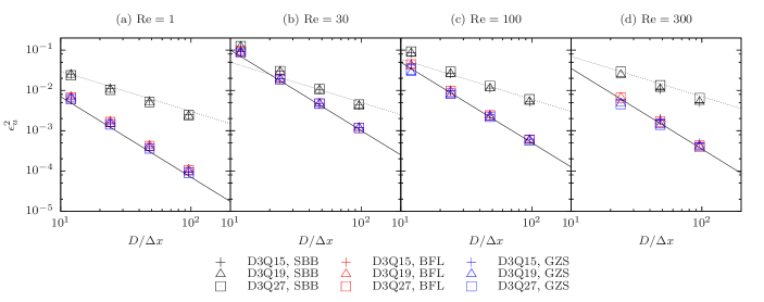
Figure 1: (Color online.) Convergence of velocity error residuals ($\epsilon^{2}_{u}$) as defined in Eq. (18) vs. diameter in lattice units. (a) Reynolds number $\mathrm{Re}=1$; (b) $\mathrm{Re}=30$; (c) $\mathrm{Re}=100$; (d) $\mathrm{Re}=300$. Colors (black, red, blue) indicate boundary condition (SBB, BFL, GZS) and shapes (crosses, triangles, squares) indicate the velocity set (D3Q15, D3Q19, D3Q27). The solid lines are guides to the eye showing first-order (dashed) and second-order (solid) convergence. The simulations with $\mathrm{Re}=300$ and $D=12\Delta x$ became unstable due to the high Mach number and are not shown.

The Junk-Yang method showed poor stability (instability being defined as one of the distribution functions becoming negative) and only producing a converged solution for the lowest resolution cases at low Reynolds number. We therefore disregard the JY method from further consideration. We do however have some confidence in our implementation of the method as our unit test suite demonstrates (data not shown) that the implementation reduces to SBB when the wall is a plane normal to one of the axes and halfway between the site and its non-fluid neighbors, as expected Junk and Yang (2005a).

In Fig. 1 we show the velocity errors as a function of increasing resolution for the remaining three boundary condition methods and the three velocity sets. We show only the results for the LBGK collision operator (the results with MRT are visually indistinguishable).

The results clearly show that SBB gives the expected first-order convergence as the resolution increases, while BFL and GZS show second-order convergence with similar prefactors. GZS offers slightly superior accuracy than BFL, reaching up to 20% lower errors ($\mathrm{Re}=300$) but the relative benefit is highly variable, vanishing in some cases.

As the Reynolds number is increased, we note that the errors also increase, particularly when going from $\mathrm{Re}=1$ to $30$. This is likely due to the increase in Mach number. The small improvement from $\mathrm{Re}=30$ to $300$ is probably due to the decreasing density difference and hence reduced compressibilty errors.

The velocity set has a small effect on the measured accuracy: D3Q15 and D3Q19 are almost coincident. D3Q27 does offer a small benefit of $1$–$4\%$ for GZS and BFL, but worsens accuracy for SBB; this may be due to the greater number of sites which have to implement the boundary condition and therefore suffer from the first-order modeling error.

III.3 Womersley flow

Here we report on simulations of oscillatory flow, in order to explore the different boundary condition methods’ effect on accuracy for time-dependent cases. The Womersley number ($\alpha$) is a dimensionless number governing dynamical similarity in cases of oscillatory flow. It relates to the ratio of transient forces to viscous forces (or alternatively the ratio of diameter to boundary layer growth during one period of oscillation). In the case of a cylinder (radius $R$, axis $\mathbf{\hat{n}}$) and laminar flow with zero average pressure gradient ($\partial_{n}p(t)=(A/L)\sin{\omega t}$, $\omega\equiv 2\pi/T_{\mathrm{osc}}$), it is defined as:

$$\alpha=R\sqrt{\frac{\omega}{\nu}},$$ (19)

where $\nu$ is the fluid viscosity. The time-dependent Navier-Stokes equations admit an analytic solution Formaggia et al. (2009):

$$\mathbf{u}(r,t)=-\Re\left(\frac{A}{\omega\rho L}\left[1-\frac{J_{0}(i^{3/2}\alpha\frac{r}{R})}{J_{0}(i^{3/2}\alpha)}\right]e^{i\omega t}\right)\mathbf{\hat{n}},$$ (20)

where $J_{0}$ is the order-0 Bessel function of the first kind and $\Re(z)$ gives the real part of $z$.

Table 2: Parameters for Womersley flow simulations. All values are given in lattice units. Parameters are: Reynolds number (defined for a Poiseuille flow with the maximum pressure gradient); Womersley number; predicted Mach number (based on the maximum Poiseuille flow); the LBGK relaxation time; the maximum relative density difference; the period of the pressure oscillation, and the momentum diffusion time.

$Re$	$\alpha$	$\mathrm{Ma}$	$\tau$	$\Delta\rho/\rho_{0}$	$T_{\mathrm{osc}}$	$T_{\mathrm{mom}}$	$T_{s}$
$30$	$4$	$0.043$	$0.620$	$0.0040$	$5656$	$57600$	$333$
$100$	$8$	$0.078$	$0.565$	$0.0039$	$2608$	$107000$	$333$
$300$	$12$	$0.113$	$0.531$	$0.0027$	$2432$	$223000$	$333$

In the larger arteries of the human body, Womersley numbers range approximately between 4 and 20 Bronzino (2006), so we select from this range. For these simulations, we define the Reynolds number as that for a Poiseuille flow with a pressure gradient given by the amplitude of the imposed gradient. Based on measured Reynolds and Womersley numbers in human arteries Bronzino (2006), we have fit a simple power law $\alpha=A\mathrm{Re}^{\gamma}$, giving $\gamma=0.36$ and $A=0.1$. We select parameters only from this curve within the $\mathrm{Re}-\alpha$ plane, as shown in Table 2. We use the same cylinder orientation as in Sec. III.2 and select a diameter $D=48\Delta x$, as this gives a reasonable balance between computational cost and accuracy, such as would be chosen for production simulations; we keep $L=4D$. We initialize the simulation to a constant pressure with zero velocity (with the phase of the pressure oscillation chosen such that the driving difference is zero at simulation start). We allow the simulation to run until $\Delta u(t,t-T_{\mathrm{osc}})<10^{-7}$ is reached for all sample points during one oscillation; however, to reduce the amount of data collected, we record data only for those points within one lattice unit of an axis-normal plane halfway along the cylinder. This was reached in 6 to 25 oscillation periods.

We run these simulations for all combinations of LBM components and compute residuals at four sample points during one pressure oscillation period using Eq. (18). The four residuals are then reduced by taking the root-mean-square average and the maximum respectively, effectively extending the averaging/maximization over time as well as space. We estimate the maximum as the maximum velocity over a full period at the centre of the pipe, i.e.,

$$U_{\textrm{W}}=\frac{A}{\omega\rho L} \left\|1-\frac{1}{J_{0}(i^{3/2}\alpha)}\right\|$$

$$=\frac{4}{\alpha^{2}} \left\|1-\frac{1}{J_{0}(i^{3/2}\alpha)}\right\|U_{\textrm{max}}$$ (21)

where $U_{\mathrm{max}}$ is the maximum velocity of a Poiseuille flow driven by a pressure gradient of the amplitude of the Womersley flow.

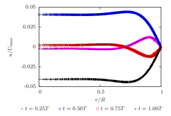
Figure 2: (Color online) Simulated (D3Q15, LBGK, BFL) axial velocity (normalized by $U_{\mathrm{max}}$) versus the radial coordinate. The Womersley number $\alpha=12$ and the Reynolds number $\mathrm{Re}=300$. The data is shown at four moments during the pulsatile cycle: $t=T/4$ (magenta, maximum positive pressure gradient), $T/2$ (blue, zero pressure gradient), $3T/4$, (red, maximum negative pressure gradient) $T$ (black, zero pressure gradient). The analytical solutions are shown with solids lines.

Table 3: Error residuals for pulsatile flow simulations with different LBM components. On the left are the boundary condition method (BC); collision operator (CO); and velocity set (DmQn). On the right are the error residuals $\epsilon^{2}_{u}$ for different values of Womersley number $\alpha$ (other parameters are as shown in Table 2).

			$\epsilon^{2}_{u}$
BC	CO	DmQn	$\alpha=4$	$\alpha=8$	$\alpha=12$
SBB	LBGK	D3Q15	$0.0085$	$0.0250$	$0.0343$
SBB	MRT	D3Q15	$0.0083$	$0.0248$	$0.0373$
SBB	LBGK	D3Q19	$0.0079$	$0.0234$	$0.0321$
SBB	MRT	D3Q19	$0.0090$	$0.0264$	$0.0395$
SBB	LBGK	D3Q27	$0.0089$	$0.0273$	$0.0395$
BFL	LBGK	D3Q15	$0.0013$	$0.0079$	$0.0128$
BFL	MRT	D3Q15	$0.0013$	$0.0078$	$0.0132$
BFL	LBGK	D3Q19	$0.0011$	$0.0069$	$0.0107$
BFL	MRT	D3Q19	$0.0012$	$0.0072$	$0.0118$
BFL	LBGK	D3Q27	$0.0012$	$0.0074$	$0.0124$
GZS	LBGK	D3Q15	$0.0013$	$0.0082$	$0.0139$
GZS	LBGK	D3Q19	$0.0011$	$0.0071$	$0.0115$
GZS	LBGK	D3Q27	$0.0012$	$0.0075$	$0.0128$

In Fig. 2 we show an example of the simulated velocities, for the D3Q15 velocity set, the LBGK collision operator and the BFL boundary condition. We plot the axial velocity, normalized by $U_{\mathrm{max}}$, against the radial coordinate at four evenly spaced moments during the period of oscillation. The agreement with the analytical profiles is excellent.

The $\ell^{2}$ error-norms for the simulations are shown in Table 3. We see that all simulations well approximate the analytical solutions, with errors in the range $0.1$–$4\%$. In Fig. 3, we show the range of error residuals against Womersley number. This clearly shows the the BFL and GZS methods offers superior accuracy to SBB in all cases, irrespective of the choice of collision operator and velocity set. Choosing MRT over LBGK does not offer any benefits, however we have not varied the relaxation rates for the non-stress tensor moments of the distributions (e.g., by projecting out all the kinetic modes every timestep or optimizing “magic numbers” d’Humières and Ginzburg (2009)). We note again that we have adopted the parameters from d’Humières et al. (2002) without optimization. The choice of velocity set does play a small role, especially in the higher Reynolds and Womersley number cases, leading to slightly improved results with larger velocity sets.

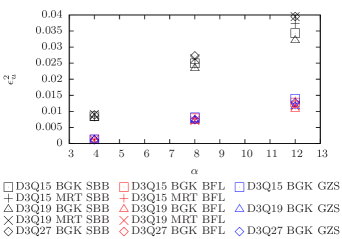
Figure 3: (Color online.) Error residuals $\epsilon^{2}_{u}$ as defined in Eq. (18) for simulations of pulsatile flow vs. Womersley number $\alpha$. Colors (black, red, blue) indicate boundary condition (SBB, BFL, GZS) and shapes the collision operator and velocity set. LBGK is indicated by polygons (square: D3Q15; triangle: D3Q19; diamond: D3Q27) and MRT by crosses ($+$: D3Q15; $\times$: D3Q19).

III.4 Dean flow

The problems in the cylinders studied above are fundamentally 2D flows. To more throroughly test the boundary conditions, we choose a further benchmark problem that is fully 3D: flow in a torus. For moderate Dean numbers (the dynamical similarity number for flow in curved pipes; see below) the primary, axial flow is a perturbation of a parabolic profile while the secondary flow in a cross sectional plane is a pair of counter-rotation vortices—see the grayscale images in Fig. 5. We define the radius of the tube as $a$ and the distance from the center of the tube to the center of the torus as $c$; our coordinate systems are illustrated in Fig. 4.

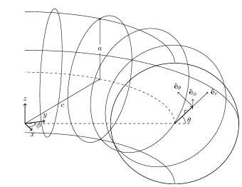
Figure 4: Parameters and coordinate systems for the torus simulations. The radius of the tube is $a$ and the distance from the center of the tube to the center of the torus is $c$. We define a toroidal coordinate system $(r,\theta,\phi)$ where $(r,\theta)$ are polar coordinates in the cross-section plane and $\phi$ is the angle that the cross-section plane makes with the $x$-$z$ plane.

The characteristic number for flow in curved pipes is the Dean number $\kappa$ given by Dean (1927, 1928)

$$\kappa=4\mathrm{Re}\sqrt{2\delta}$$ (22)

where $\mathrm{Re}$ is the Reynolds number based on the maxiumum axial velocity of the flow that would result from the same pressure gradient in a straight pipe and $\delta\equiv a/c$ is the curvature ratio. The Dean number is the square root of the product of the inertial and centrifugal forces, scaled by the viscous forces Berger et al. (1983).

Dean Dean (1927, 1928) was the first to derive an approximate solution for laminar, fully developed flow in a torus and much of the later work is reviewed in Berger et al. (1983). We choose to use the approximations for a weakly curved pipe from Siggers and Waters Siggers and Waters (2005), due to their clarity of presentation. They define the velocity components $(U_{r},U_{\theta},U_{\phi})\equiv\frac{\nu}{a}(u,v,w)$ and the stream function $\psi$ by

$$u=\frac{1}{hr}\frac{\partial(h\psi)}{\partial\theta}\mbox{ and }v=-\frac{1}{h}\frac{\partial(h\psi)}{\partial r}$$ (23)

where $h=1+\delta r\cos\theta$. They then expand as a power series in $\kappa$

$$w=\kappa\sum_{k=0}^{\infty}\kappa^{2k}w_{k}\mbox{ and }\psi=\kappa^{2}\sum_{k=0}^{\infty}\kappa^{2k}\psi_{k}$$ (24)

and each term $w_{k}$ and $\psi_{k}$ as a series in $\delta$:

$$w_{k}=\sum_{j=0}^{\infty}\delta^{j}w_{kj}\mbox{ and }\psi_{k}=\sum_{j=0}^{\infty}\delta^{j}\psi_{kj}.$$ (25)

We use only the terms

$$w_{00} = \frac{1}{4}(1-r^{2}),$$

$$w_{01} = -\frac{3}{16}r(1-r^{2})\cos\theta,$$ (26)

$$w_{02} = \frac{1}{128}(1-r^{2})(-3+11r^{2}+10r^{2}\cos 2\theta)$$

and

$$\psi_{00} = \frac{1}{2^{10}\times 3^{2}}r(1-r^{2})^{2}(4-r^{2})\sin\theta,$$

$$\psi_{01} = \frac{1}{2^{12}\times 3^{2}\times 5}r^{2}(1-r^{2})^{2}(56-17r^{2})\sin 2\theta,$$ (27)

$$\psi_{02} = \frac{1}{2^{17}\times 3^{2}\times 5}r(1-r^{2})^{2}[-(133-976r^{2}$$

$$+327r^{4})\sin\theta+2r^{2}\left(499-172r^{2}\right)\sin 3\theta].$$

This expansion is accurate for $\delta\ll 1$ and $\kappa\lesssim 100$ Siggers and Waters (2005).

For our simulations, we select a curvature $\delta=0.1$ and two target Dean $\kappa_{0}$ numbers (100 and 200), as representative of physiological values while not making the series expansion too inaccurate. The tube radius $a=24\Delta x$ (hence $c=240\Delta x$) and the shear relaxation time $\tau=0.6\Delta t$ for $\kappa_{0}=100$ and $\tau=0.55\Delta t$ for $\kappa_{0}=200$. We sample the flow at a plane half way around the torus to keep data volumes small and impose a parabolic flow profile at the inlet and a constant pressure at the outlet. Since the imposed profile is incorrect, we simulate 90% of the full torus to allow distance for the flow to fully develop. One must also compute actual Dean number, by equating the imposed flux

$$Q_{\mathrm{Pois}}=\frac{\pi a\nu\mathrm{Re}{}_{0}}{4}=\frac{\pi a\nu\kappa_{0}}{16\sqrt{2\delta}}$$ (28)

to the flux computed from Eq. (24):

$$Q_{\kappa}{} = \int_{0}^{1}\int_{0}^{2\pi}U_{\phi}a^{2}r\,\mathrm{d}r\,\mathrm{d}\theta$$ (29)

$$= \frac{\pi a\nu\kappa}{384}(48+\delta^{2}),$$

giving:

$$\kappa=\frac{12\kappa_{0}}{48+\delta^{2}}\sqrt{\frac{2}{\delta}}.$$ (30)

This gives our actual Dean numbers as $\kappa\approx 111.78$ and $\kappa\approx 223.56$. We use the $\ell^{2}$-norm error from Eq. (18) but also evaluate it for the primary flow and the seconday flow.

The simulations using the GZS boundary condition were unstable for the larger $\kappa$/$\mathrm{Re}$ case, but the remaining results are collected in Table 4, and in Fig. 5 and Fig. 6 we show streamline plots of the secondary flow, colored by the modulus of the local absolute error $\|\mathbf{u}^{\star}\|=\|\mathbf{u}-\mathbf{U}\|$ from Eq. (17), scaled by $U_{\phi}$ evaluated at the tube center, i.e.,

$$\epsilon_{\kappa}=\frac{\|\mathbf{u}-\mathbf{U}\|}{U_{\phi}(0,0)}.$$ (31)

The table of error norms shows that the error is dominated by the error in the secondary flow, which is approximately independent of the LBM model used. This is borne out by Fig. 5 and Fig. 6 which show the patterns of the secondary flow error (i.e., the coloring) remaining near-constant. The $\kappa\approx 224$ case has much larger errors that vary little which we ascribe to the series solution becoming inaccurate.

We note that our simulations do locate the centers of the pair of vortices accurately. The streamlines for the SBB simulations show large errors in the velocity field’s direction near the walls, due to the stair casing of the boundary. This is likely to cause the stress near the walls, which is a key hemodynamic factor, to have larger errors. The primary flow errors for the case $\kappa\approx 112$ are approximately $25\%$ larger for SBB than for either BFL or GZS, again, due to the staircasing of the boundary. The velocity set and collision operator do not strongly affect the measured error, but there is a small benefit to using MRT over LBGK and for using the larger velocity sets.

Table 4: Error residuals for flow in a toroidal pipe with different LBM components. On the left are the velocity set (DmQn) and collision operator (CO). On the right are the error residuals $\epsilon^{2}_{u}$ for different boundary collision methods for the secondary flow ($\epsilon^{2}_{\mathrm{plane}}$), the primary flow ($\epsilon^{2}_{\mathrm{axial}}$) and the overall ($\epsilon^{2}_{\mathrm{all}}$).

		SBB			BFL			GZS
DmQn	CO	$\epsilon^{2}_{\mathrm{plane}}$	$\epsilon^{2}_{\mathrm{axial}}$	$\epsilon^{2}_{\mathrm{all}}$	$\epsilon^{2}_{\mathrm{plane}}$	$\epsilon^{2}_{\mathrm{axial}}$	$\epsilon^{2}_{\mathrm{all}}$	$\epsilon^{2}_{\mathrm{plane}}$	$\epsilon^{2}_{\mathrm{axial}}$	$\epsilon^{2}_{\mathrm{all}}$
		$\kappa\approx 112$, $\mathrm{Re}\approx 200$
D3Q15	LBGK	$0.076$	$0.022$	$0.079$	$0.076$	$0.018$	$0.078$	$0.076$	$0.018$	$0.079$
D3Q15	MRT	$0.076$	$0.021$	$0.079$	$0.076$	$0.018$	$0.078$	-
D3Q19	LBGK	$0.075$	$0.020$	$0.078$	$0.076$	$0.017$	$0.078$	$0.076$	$0.017$	$0.078$
D3Q19	MRT	$0.075$	$0.021$	$0.078$	$0.076$	$0.017$	$0.078$	-
D3Q27	LBGK	$0.076$	$0.022$	$0.079$	$0.076$	$0.017$	$0.078$	$0.076$	$0.017$	$0.078$
		$\kappa\approx 224$, $\mathrm{Re}\approx 400$
D3Q15	LBGK	$0.153$	$0.058$	$0.164$	$0.152$	$0.059$	$0.163$	-
D3Q15	MRT	$0.153$	$0.057$	$0.164$	$0.152$	$0.059$	$0.163$	-
D3Q19	LBGK	$0.152$	$0.059$	$0.163$	$0.152$	$0.058$	$0.163$	-
D3Q19	MRT	$0.151$	$0.060$	$0.163$	$0.152$	$0.058$	$0.162$	-
D3Q27	LBGK	$0.152$	$0.059$	$0.163$	$0.152$	$0.058$	$0.163$	-

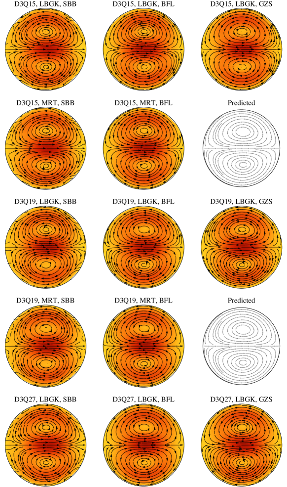
Figure 5: (Color online.) Streamlines for the secondary flow and color maps of the modulus of the error field in a torus, with Dean number $\kappa\approx 112$ and Reynolds number $\mathrm{Re}\approx 200$. The inside of the pipe is on the left of the figure. Across columns, we vary the boundary condition (SBB, BFL and GZS from left to right). Down the rows, we vary the combination of velocity set at collision operator (D3Q15+LBGK, D3Q19+LBGK, D3Q15+MRT, D3Q19+MRT, D3Q27+LBGK from top to bottom). The figures in color show the simulated results. The color field indicates the absolute error Eq. (31) where light gray (yellow online) is zero and dark (red online) is $0.15U_{\phi}(0,0)$. Since the combination of MRT and GZS is unavailable, we use these spaces to show the predicted secondary flow calculated using Eqs. (23)–(III.4) in grayscale.

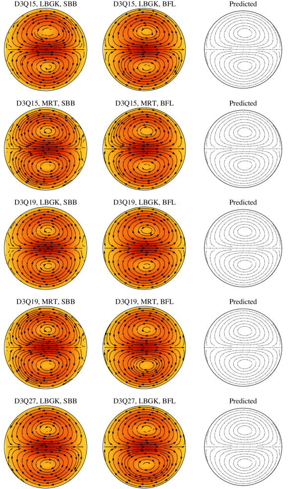
Figure 6: (Color online.) Streamlines for the secondary flow and color maps of the modulus of the error field in a torus, with Dean number $\kappa\approx 224$ and Reynolds number $\mathrm{Re}\approx 400$. The inside of the pipe is on the left of the figure. Across columns, we vary the boundary condition (SBB, BFL and GZS from left to right). Down the rows, we vary the combination of velocity set at collision operator (D3Q15+LBGK, D3Q19+LBGK, D3Q15+MRT, D3Q19+MRT, D3Q27+LBGK from top to bottom). The figures in color show the simulated results. The color field indicates the absolute error Eq. (31) where light gray (yellow online) is zero and dark (red online) is $0.3U_{\phi}(0,0)$. Since the GZS simulations were unstable, we use these spaces to show the predicted secondary flow calculated using Eqs. (23)–(III.4) in grayscale.

III.5 Relative performance

The relative performance of the options is germane to the choice of which combination of lattice-Boltzmann components to use. In Table 5 we give the measured per-core performance for the lowest $\mathrm{Re}$/$\alpha$ pulsatile flow simulations. All these runs were performed on HECToR, a Cray XE6 supercomputer with two 16-core AMD Opteron 2.3 GHz Interlagos processors per node. The simulations used 64 cores. The performance is given in millions of site updates per second (MSUPS) and is based on timings that include only the lattice-Boltzmann updates. We also estimate the relative time to perform one site update for the different methods, assuming that an SBB site update takes the same time as a bulk fluid site update. The simulation domain includes 347,401 sites of which 42,340 (12%) are at the solid-fluid boundary and hence use the various boundary condition methods.

Table 5: Performance per core for different combinations of boundary condition, collision operator and velocity set. The columns indicate the combination of collision operator and velocity set, while the rows indicate the boundary condition. Omitted simulations are indicated with a dash (-). The values are given in millions of site updates per second (MSUPS) followed by the time to perform one boundary condition site update, relative to SBB, in parentheses.

	LBGK						MRT
	D3Q15		D3Q19		D3Q27		D3Q15		D3Q19
SBB	1.5	(1)	1.2	(1)	0.8	(1)	0.8	(1)	0.5	(1)
BFL	1.4	(1.6)	1.2	(1.4)	0.8	(1.3)	0.8	(1.3)	0.5	(1.2)
GZS	1.0	(4.9)	0.8	(5.1)	0.5	(6.1)	-		-

SBB gives the best computational performance in all cases while BFL requires between $20\%$ and $60\%$ more compute time; the extra time needed remains approximately constant across all collision operators and velocity sets, but reduces as a fraction of the time to perform a bulk site update. GZS requires approximately five times the computational effort compared to a bulk site.

For the three velocity sets, the number of distribution updates per second (i.e., $\mathrm{SUPS}\times Q$) remains approximately constant—D3Q15: $22.5$; D3Q19: $22.8$; D3Q27: $21.6$. The cost of changing the collision operator from LBGK to MRT is large, decreasing performance by a factor of two. We do not place much emphasis on this result as the MRT collision operator is implemented naïvely and there is scope to improve the performance.

IV Conclusion

The majority of benchmark problems reported in the lattice-Boltzmann literature use lattice-aligned geometries, rather than the complex domains required by many applications. We have performed a comparison between LBM simulation solutions, from our open source application HemeLB hem , and analytical solutions in a non-lattice-aligned, curved domain up to Reynolds numbers of 300, with steady and unsteady flow. We have varied the resolution of the grid used and the different components of the algorithm (collision operator, velocity set, no-slip boundary condition). We find that at these moderate values of $\mathrm{Re}$, the choice of velocity set and collision operator do not greatly affect accuracy or stability, but that the choice of no-slip boundary condition method is critical.

Recent studies White and Chong (2011); Kang and Hassan (2012) have shown that the commonly used D3Q15 and D3Q19 velocity sets can give strongly orientation (with respect to the underlying lattice) dependent results when simulating flows for Reynolds numbers $\geq 250$, while the D3Q27 velocity set maintains good isotropy. The problems studied are in relatively complex cases (a circular pipe with a narrowing; circular and square pipes at higher Reynolds number) but they are comparable to our simulations of flow in a toroidal pipe due to the strong three-dimensionality of the Dean flow. We do not see any lattice artifacts in these simulations, even with $\mathrm{Re}\approx 400$ and the strong secondary flows. Even so, one must be aware of the possibility of anisotropy when simulating a complex flow and ensure that it does not occur in one’s work.

The Junk-Yang method shows poor stability and is therefore unsuitable for our hemodynamic applications or other applications that require even moderate Reynolds numbers.

Simple bounce-back (SBB) shows first-order convergence over a wide range of resolutions and Reynolds numbers, as expected. We confirm that the Bouzidi-Firdaouss-Lallemand (BFL) and (modified) Guo-Zheng-Shi (GZS) methods both show second-order convergence over a wide range of resolutions and Reynolds numbers. For the steady flow problem, GZS has lower errors than BFL, by a variable amount (up to 20%). For the time-dependent problem, BFL has lower errors than GZS, by around 10%. GZS also became unstable for the largest Reynolds number flows in curved pipes.

The typical goal of most computational modeling is to solve the desired system of equations to some problem-dependent accuracy in the minimum time. Considering the steady flow problem as a proxy, we can estimate which of the GZS and BFL boundary conditions will give the shortest simulation time. Taking an average increase in accuracy for GZS of $\sim 10\%$, allows us to estimate that the GZS method can use a $\sim 5\%$ lower resolution to obtain the same accuracy. Due to the diffusive scaling of the timestep, the GZS method will require fewer site updates than BFL by a factor of $\sim 0.95^{5}\approx 0.79$ or $21\%$ less. However the BFL method is more computationally efficient, by $\sim 30\%$, for the typical surface:bulk ratios studied here, so the equivalent-accuracy BFL simulation will complete sooner

We therefore recommend BFL as the best all-round boundary condition of those tested, due to to the good accuracy, performance, stability and simplicity of implementation. The GZS method also offers good accuracy (in our modified form) but has worse stability at high Reynolds number and much poorer performance. This last point may not matter in domains with a relatively low number of wall boundary sites. SBB is much less accurate, but may be acceptable for use in undemanding applications and when development time is at a premium. We believe that these results will prove helpful to the community when selecting methods for simulating hemodynamics and comparable applications with lattice-Boltzmann methods.