Performance Evaluation of Random Set Based Pedestrian Tracking Algorithms

Abstract

The paper evaluates the error performance of three random finite set based multi-object trackers in the context of pedestrian video tracking. The evaluation is carried out using a publicly available video dataset of 4500 frames (town centre street) for which the ground truth is available. The input to all pedestrian tracking algorithms is an identical set of head and body detections, obtained using the Histogram of Oriented Gradients (HOG) detector. The tracking error is measured using the recently proposed OSPA metric for tracks, adopted as the only known mathematically rigorous metric for measuring the distance between two sets of tracks. A comparative analysis is presented under various conditions.

I Introduction

Random set theory has recently been proposed as a mathematically elegant framework for Bayesian multi-object filtering [1]. Research within this theoretical framework has resulted in new multi-object filtering algorithms, such as the probability density hypothesis (PHD) filter [2], Cardinalised PHD filter [3], and Multi-Bernoulli filter [1, 4]. The main feature of multi-object filters is that they estimate sequentially the number of objects in the surveillance volume of interest (the so-called cardinality) and their states in the state space. Formulation of multi-object trackers from random-set based multi-object filters has attracted a lot of interest recently, see e.g. [5, 6, 7, 8]. The output of a tracker is a set of tracks, that is, labeled temporal sequences of state estimates associated with the same object.

(a)

.

(b)

Figure 1: Frame 320 from the dataset used in performance evaluation: (a) Head and body detections (yellow and cyan rectangles, respectively); (b) tracker output (the result of recursive processing of 79 previous frames and the current frame); track trajectories indicated by white lines; red lines are velocity vectors; squares indicate the heads of pedestrians

In this paper we adopt the “tracking-by-detection” approach to pedestrian tracking, which has become very popular in computer vision due to its applicability to moving un-calibrated cameras [9, 10]. Typically pedestrian detections are obtained using the Histogram of Oriented Gradients (HOG) detector [11], trained using either head images (for head detections) or body images (for body detections). An example of head and body detections is shown in Fig.1.(a). Head and body detections are unreliable in the sense that: (1) not all pedestrians are detected in every frame; (2) the chance of false detections is quite real, with the spatial density of false detections typically non-uniform. This is evident in Fig.1.(a).

If the state vector of each object (pedestrian) contains the position (e.g. the head centroid), but not the size of the object, then both the head and body detections are instances of imprecise measurements: they represent rectangular regions (two-dimensional intervals) within which the true object is possibly located. As such, they can be modelled as random closed sets (rather than random variables). The first tracking algorithm considered in the paper is designed specifically for imprecise measurements: it represents a multi-object tracker built from the Bernoulli filter described in [12]. We will refer to this tracker as Algorithm 1.

An imprecise measurement (e.g. an interval in the measurement space) can always be converted to a precise but random measurement (e.g. a point in the measurement space which is affected by additive noise). The two remaining algorithms considered in the paper assume precise random detections of heads/bodies for pedestrian tracking. Algorithm 2 is the same as Algorithm 1, but using the precise random (Gaussian) measurements model. Algorithm 3 is based on the Cardinalised PHD filter with data association [13].

Evaluation of multi-object tracking performance has been one of the main stumbling blocks in advancing the scientific field of target tracking. A large number of evaluation measures have been proposed, both in the general context (e.g. [14, 15]) and specifically for video surveillance (e.g. [16, 17, 18, 19]). At present there is no consensus in sight on the preferred common approach. In this paper tracking error will be measured using the recently formulated Optimal sub-pattern assignment (OSPA) metric for tracks (or OSPA-T) [20]. The OSPA-T metric has an important advantage over all above mentioned performance metrics: it is a mathematically rigorous metric (it satisfies the axioms of a metric) for measuring the distance between two sets of tracks (i.e. between the ground truth and the tracker output). OSPA-T is also consistent with intuition, as discussed in [21].

The remainder of the paper is organised as follows. Section II describes the performance evaluation framework: the video dataset, the method of pre-processing detections and the OSPA-T metric. Section III reviews the three random-set based tracking algorithms. Section IV presents the experimental results under various conditions, while the conclusions of this study are drawn in Section V.

II Performance evaluation framework

II-A Video dataset and detections

The video dataset and the (hand labelled) ground truth are downloaded from the website [22]. The dataset is a video of an occasionally busy town centre street (the average number of pedestrians visible at any time is 16). The video was recorded in high definition ($1920\times 1080$ pixels at $25$ fps). Only the first 4500 frames of the video are used in the performance evaluation. Frame number 320 of the dataset is shown in Fig.1.

Head detection and pedestrian body detection algorithms were applied to each frame in the video sequence. The fastHOG GPU implementation [23] of the Histogram of Oriented Gradients (HOG) detection algorithm [11] was used for both detectors. The HOG detector applies a sliding window to the image at a regular grid of locations and scales, and classifies each sub-window as containing or not containing an object (head or pedestrian). Classification is performed using a pre-trained linear Support Vector Machine, the input to which is a set of block-wise histograms of image gradient orientation. A classification threshold of 0.75 was used for both detectors. Sliding window detectors tend to give multiple detections for one object due to their tolerance to shift and scale, so a post-processing step groups overlapping detections.

The head and pedestrian (whole body) detections have some complementary characteristics. The detector is only partially tolerant to occlusions, so the head detector tends to have a higher probability of detection since heads are generally more visible than whole bodies in surveillance video. However pedestrian textures are more distinctive than head textures, so the head detector tends to have a higher false alarm rate, picking up on round-ish background objects such as clocks and signs. The pedestrian detector is more able to detect people at a distance where the head becomes too small in the image.

Head and body detections are treated as if they are independent. Each tracker can then be regarded as a centralised multi-source fusion node, where one source of detections is the head detector while the other is the body detector. The rectangles corresponding to body detections are converted to head-like detections as follows. Suppose a body detection rectangle is specified by its upper-left corner $(\chi_{b},\eta_{b})$, width $w_{b}$ and height $h_{b}$. Then for its corresponding head-like detection, the upper-left corner coordinates are computed as: $\chi^{\prime}_{h}=\chi_{b}+0.325\,w_{b}$ and $\eta^{\prime}_{h}=\eta_{b}+0.09\,h_{b}$, while the width and height are $w^{\prime}_{h}=0.35\,w_{b}$ and $h^{\prime}_{h}=0.19\,h_{b}$, respectively.

II-B OSPA-T metric

Traditional multi-object tracking performance measures describe various aspects of tracking performance, such as timeliness (e.g. track initiation delay, track overshoot), track accuracy (e.g. position, heading, velocity error), track continuity (e.g. track fragmentation, track labelling swaps) and false tracks (their count and duration). These measures are based on heuristic, and it is unclear how to combine them into a single score because they are correlated.

OSPA-T [20] is defined as a theoretically rigorous distance measure on the space of finite sets of tracks, and it has been proven that it satisfies the axioms of a metric. The computation of OSPA-T is described in Table I. Suppose we are given two sets of tracks, the ground truth tracks $\{X^{(1)},\dots,X^{(L)}\}$ and estimated tracks $\{Y^{(1)},\dots,Y^{(R)}\}$. A track $X^{(l)}$, $l=1,\dots,L$, is defined as a temporal sequence $X^{(l)}=(X_{1}^{(l)},\dots,X_{K}^{(l)})$ where each $X^{(l)}_{k}$, $k=1,\dots,K$, is either an empty set (if track does not exist at time $k$) or a singleton whose element is $(l,\mathbf{x}_{k})$. Here $l\in\mathbb{N}$ is the track label and $\mathbf{x}_{k}$ is its state at time $k$. The labels of ground truth tracks are by convention adopted to be $1,2,\dots,L$.

The first step in the computation of OSPA-T is to label the estimated tracks (steps 3,4 and 5 in Table I). This first involves finding the best assignment $\lambda^{*}$ of $R$ estimated tracks to $L$ ground truth tracks. An assignment is a mapping $\lambda^{*}(\ell)\in\emptyset\cup\{1,\dots,R\}$, for $\ell=1,\dots,L$. This is typically carried out using a two-dimensional assignment algorithm, such as the auction or Munkres algorithm [24]. If for an estimated track $r=1,\dots,R$ exists a true track $\ell$ such that $\lambda^{*}(\ell)=r$, then track $r$ is assigned label $\ell$. Estimated tracks which remain unassigned according to $\lambda^{*}$ are given labels different from all true track labels (i.e. integers greater than $L$).

Then, for each time step $k=1,\dots,K$, the OSPA distance between the two labeled sets:

$$\mathfrak{X}_{k} = \{(l_{1},\mathbf{x}_{k,1}),\dots,(l_{m},\mathbf{x}_{k,m})\}$$ (1)

$$\mathfrak{Y}_{k} = \{(s_{1},\mathbf{y}_{k,1}),\dots,(s_{n},\mathbf{y}_{k,n})\}$$ (2)

is computed. The set $\mathfrak{X}_{k}$ represents the set of existing ground truth labeled track states at time $k$; similarly $\mathfrak{Y}_{k}$ is the set of existing estimated labeled track states at time $k$. The OSPA distance between these two labeled sets is computed as [20]:

$$D (\mathfrak{X}_{k},\mathfrak{Y}_{k})=$$

$$\left[\frac{1}{n}\left(\min_{\pi\in\Pi_{n}}\sum_{i=1}^{m}\Big{(}d_{c}\big{(}\tilde{\mathbf{x}}_{k,i},\tilde{\mathbf{y}}_{k,\pi(i)}\big{)}\Big{)}^{p}+(n-m)\cdot c^{p}\right)\right]^{1/p}$$ (3)

where $\tilde{\mathbf{x}}_{k,i}\equiv(l_{i},\mathbf{x}_{k,i})$, $\tilde{\mathbf{y}}_{k,\pi(i)}\equiv(s_{\pi(i)},\mathbf{y}_{k,\pi(i)})$ and

• $d_{c}(\tilde{\mathbf{x}},\tilde{\mathbf{y}})=\min(c,d(\tilde{\mathbf{x}},\tilde{\mathbf{y}}))$ is the cut-off distance between two tracks at $t_{k}$, with $c>0$ being the cut-off parameter;

• $d(\tilde{\mathbf{x}},\tilde{\mathbf{y}})$ is the base distance between two tracks at $t_{k}$;

• $\Pi_{n}$ represents the set of permutations of length $m$ with elements taken from $\{1,2,\dots,n\}$;

• $p\in[1,\infty)$ is the OSPA metric order parameter.

For the case $m>n$, the definition is $D_{p,c}(\mathfrak{X}_{,}\mathfrak{Y})=D_{p,c}(\mathfrak{Y}_{k},\mathfrak{X}_{k})$. If both $\mathfrak{X}_{k}$ and $\mathfrak{Y}_{k}$ are empty sets (i.e. $m=n=0$), the distance is zero.

TABLE I: Computation Steps of OSPA-T Metric

 

1:function OSPA-T($\{X^{(1)},\dots,X^{(L)}\},\{Y^{(1)},\dots,Y^{(R)}\}$)

2:    $\%$ Label the estimated tracks

3:    For $j=1,\dots,R$, Label$[Y^{(j)}]=I$ (where $I>L$)

4:    Find $\lambda^{*}$, the globally best assignment of tracks $\{X^{(1)},\dots,X^{(L)}\}$ to $\{Y^{(1)},\dots,Y^{(R)}\}$

5:    For $i=1,\dots,L$, Label$[Y^{(\lambda^{*}(i))}]=\mbox{Label}[X^{(i)}]$

6:    $\%$ Compute the distance

7:    For $k=1,\dots,K$

8:          Form the labeled sets at $t_{k}$:

9:             -Ground truth: $\mathfrak{X}_{k}=\{(l_{1},\mathbf{x}_{k,1}),\dots,(l_{m},\mathbf{x}_{k,m})\}$

10:             -Estimated: $\mathfrak{Y}_{k}=\{(s_{1},\mathbf{y}_{k,1}),\dots,(s_{n},\mathbf{y}_{k,n})\}$

11:          Compute the OSPA distance between $\mathfrak{X}_{k}$ and $\mathfrak{Y}_{k}$

12:end function

 

The base distance $d(\tilde{\mathbf{x}},\tilde{\mathbf{y}})$ is defined as:

$$d(\tilde{\mathbf{x}},\tilde{\mathbf{y}})=\Big{(}d_{\ell}(\mathbf{x},\mathbf{y})^{p^{\prime}}+d_{\alpha}(l,s)^{p^{\prime}}\Big{)}^{1/p^{\prime}},$$ (4)

where: $p^{\prime}\in[1,\infty)$ is the base distance order parameter; $d_{\ell}(\mathbf{x},\mathbf{y})$ is the localisation base distance, typically adopted as the $p^{\prime}$-norm: $d_{\ell}(\mathbf{x},\mathbf{y})=\|\mathbf{x}-\mathbf{y}\|_{p^{\prime}}$; $d_{\alpha}(l,s)$ is the labeling error, adopted as: $d_{\alpha}(s,t)=\alpha\,\bar{\delta}[s,t]$, where $\bar{\delta}[i,j]$ is the complement of the Kroneker delta, that is $\bar{\delta}[i,j]=0$ if $i=j$, and $\bar{\delta}[i,j]=1$ otherwise. Parameter $\alpha\in[0,c]$ here controls the penalty assigned to the labeling error $d(s,t)$ interpreted relative to the localisation distance $d_{\ell}(\mathbf{x},\mathbf{y})$. The case $\alpha=0$ assigns no penalty, and $\alpha=c$ assigns the maximum penalty.

Since in this paper we consider a sequence of a large number of frames ($K=4500$), the OSPA-T is applied over non-overlapping segments (blocks) of frames.

II-C Base distance is a metric

The base distance $d(\tilde{\mathbf{x}},\tilde{\mathbf{y}})$, defined in (4), satisfies the three axioms of a metric: identity, symmetry and triangle inequality. To prove identity and symmetry is trivial. The proof of triangle inequality, presented in [20, Sec.III.A], is wrong and this section presents the correct proof.

Let $\tilde{\mathbf{x}}=\left(l,\mathbf{x}\right)$, $\tilde{\mathbf{y}}=\left(s,\mathbf{y}\right)$, $\tilde{\mathbf{z}}=\left(u,\mathbf{z}\right)$. The following proof for the triangle inequality is given in [20, Sec III.A]

$$d\left(\mathbf{\tilde{x}},\mathbf{\tilde{y}}\right)^{p}\leq d\left(\mathbf{\tilde{x}},\mathbf{\tilde{z}}\right)^{p}+d\left(\mathbf{\tilde{z}},\mathbf{\tilde{y}}\right)^{p}$$ (5)

where in Sec.II-B and [20] notation $p^{\prime}$ was used instead of $p$. Equation (5) is wrong and this can be seen for example by adopting: $p=2$, $\mathbf{\tilde{x}}=\left(1,0\right)$, $\mathbf{\tilde{y}}=\left(1,5\right)$, $\mathbf{\tilde{z}}=\left(1,4.99\right)$. Then $d\left(\mathbf{\tilde{x}},\mathbf{\tilde{y}}\right)^{p}=25$ and $d\left(\mathbf{\tilde{x}},\mathbf{\tilde{z}}\right)^{p}+d\left(\mathbf{\tilde{z}},\mathbf{\tilde{y}}\right)^{p}\approx 24.90$. Moreover, (5) does not prove the triangle inequality.

We want to prove that

$$d\left(\tilde{\mathbf{x}},\tilde{\mathbf{y}}\right)\leq d\left(\tilde{\mathbf{x}},\tilde{\mathbf{z}}\right)+d\left(\tilde{\mathbf{z}},\tilde{\mathbf{y}}\right)$$ (6)

where according to (4)

$$d\left(\tilde{\mathbf{x}},\tilde{\mathbf{y}}\right)^{p}=d_{\ell}\left(\mathbf{x},\mathbf{y}\right)^{p}+\alpha^{p}\overline{\delta}\left[l,s\right].$$ (7)

As $d_{\ell}\left(\cdot,\cdot\right)$ is a metric, it meets the triangle inequality

$$d_{\ell}\left(\mathbf{x},\mathbf{y}\right)\leq d_{\ell}\left(\mathbf{x},\mathbf{z}\right)+d_{\ell}\left(\mathbf{z},\mathbf{y}\right)$$ (8)

As both sides of the inequality are positive numbers and $p\geq 1$

$$d_{\ell}\left(\mathbf{x},\mathbf{y}\right)^{p}\leq\left(d_{\ell}\left(\mathbf{x},\mathbf{z}\right)+d_{\ell}\left(\mathbf{z},\mathbf{y}\right)\right)^{p}$$ (9)

We also have that

$$\alpha\overline{\delta}\left[l,s\right]\leq\alpha\overline{\delta}\left[l,u\right]+\alpha\overline{\delta}\left[u,s\right]$$ (10)

As both sides of inequality (10) are positive and $p\geq 1$

$$\left(\alpha\overline{\delta}\left[l,s\right]\right)^{p}\leq\left(\alpha\overline{\delta}\left[l,u\right]+\alpha\overline{\delta}\left[u,s\right]\right)^{p}$$ (11)

Using (9) and (11)

$$d_{\ell} \left(\mathbf{x},\mathbf{y}\right)^{p}+\left(\alpha\overline{\delta}\left[l,s\right]\right)^{p}\leq$$

$$\bigg{(}d_{\ell}\left(\mathbf{x},\mathbf{z}\right)+d_{b}\left(\mathbf{z},\mathbf{y}\right)\bigg{)}^{p}+\bigg{(}\alpha\overline{\delta}\left[l,u\right]+\alpha\overline{\delta}\left[u,s\right]\bigg{)}^{p}$$ (12)

that is

$$\sqrt[p]{d_{\ell}\left(\mathbf{x},\mathbf{y}\right)^{p}+\left(\alpha\overline{\delta}\left[l,s\right]\right)^{p}}\leq$$

$$\sqrt[p]{\left(d_{\ell}\left(\mathbf{x},\mathbf{z}\right)+d_{\ell}\left(\mathbf{z},\mathbf{y}\right)\right)^{p}+\left(\alpha\overline{\delta}\left[l,u\right]+\alpha\overline{\delta}\left[u,s\right]\right)^{p}}$$ (13)

As $p\geq 1$, using the Minkowski inequality [25] on the right hand side of (13)

$$\sqrt[p]{\left(d_{\ell}\left(\mathbf{x},\mathbf{z}\right)+d_{\ell}\left(\mathbf{z},\mathbf{y}\right)\right)^{p}+\left(\alpha\overline{\delta}\left[l,u\right]+\alpha\overline{\delta}\left[u,s\right]\right)^{p}}\leq$$

$$\sqrt[p]{d_{\ell}\left(\mathbf{x},\mathbf{z}\right)^{p}+\alpha^{p}\overline{\delta}\left[l,u\right]}+\sqrt[p]{d_{\ell}\left(\mathbf{z},\mathbf{y}\right)^{p}+\alpha^{p}\overline{\delta}\left[u,s\right]}$$ (14)

Finally, using (13) and (14), we get

$$\sqrt[p]{d_{\ell}\left(\mathbf{x},\mathbf{y}\right)^{p}+\alpha^{p}\overline{\delta}\left[l,s\right]}\leq$$

$$\sqrt[p]{d_{\ell}\left(\mathbf{x},\mathbf{z}\right)^{p}+\alpha^{p}\overline{\delta}\left[l,u\right]}+\sqrt[p]{d_{\ell}\left(\mathbf{z},\mathbf{y}\right)^{p}+\alpha^{p}\overline{\delta}\left[u,s\right]}$$ (15)

The proof is finished using (7):

$$d\left(\mathbf{\tilde{x}},\mathbf{\tilde{y}}\right)\leq d\left(\mathbf{\tilde{x}},\mathbf{\tilde{z}}\right)+d\left(\mathbf{\tilde{z}},\mathbf{\tilde{y}}\right).$$ (16)

III Description of Algorithms

The state vector of a single object is adopted for all algorithms as $\mathbf{x}=\left[\begin{matrix}x&\dot{x}&y&\dot{y}\end{matrix}\right]^{\intercal}$, where $(x,y)$ is the position (in pixels) of the pedestrian head centroid and $(\dot{x},\dot{y})$ is its velocity vector (in pixels/s). The number of objects from frame to frame varies. The random finite set of head detections at frame $k$ is denoted $Z_{k}^{(1)}$. Accordingly, the random set of head-like body detections (see the explanation in the last sentence of Sec.II-A) is $Z_{k}^{(2)}$.

Algorithms 1 and 2 are based on the multi-sensor Bernoulli filter [26], where the “sensors” are the two types of pedestrian head detections. Separate and independent Bernoulli filters are run for each target. Target interactions are taken care of by the appropriately increased clutter intensity, as in [27]. This multi-object tracking algorithm has been described in some detail in [28]. The difference between Algorithms 1 and 2 is in the model of the single-object likelihood function. Let $\mbox{\boldmath$\zeta$}\in Z_{k}^{(i)}$, for $i=1,2$, be a detection resulting from an object (i.e. a pedestrian head) in the state $\mathbf{x}$. A head detection is a rectangle, thus $\zeta$ is specified by a tuple $(\chi,\eta,w,h)$, where $(\chi,\eta)$ determines its upper-left corner, while $w$ and $h$ are the width and height, respectively.

The single-object likelihood function used in Algorithm 1 treats the detection $\zeta$ as an imprecise measurement and is defined as in [12]:

$$g_{k}^{(i)}(\zeta|\mathbf{x})=\varphi(\mathbf{H}\mathbf{x};\underline{\zeta},\mathbf{\Sigma}^{(i)})-\varphi(\mathbf{H}\mathbf{x};\overline{\zeta},\mathbf{\Sigma}^{(i)})$$ (17)

where $\varphi(\mathbf{z};\mu,\mathbf{\Sigma}^{(i)})$ is the Gaussian cumulative distribution function with mean $\mu$ and covariance $\mathbf{\Sigma}^{(i)}=\mbox{diag}[{\sigma_{x}^{(i)}}^{2},\;{\sigma_{y}^{(i)}}^{2}]$; $\underline{\zeta}$ and $\overline{\zeta}$ are the lower and upper bound of the rectangle, and $\mathbf{H}=\left[\begin{matrix}1&0&0&0\\ 0&0&1&0\end{matrix}\right]$. If $\sigma_{x}^{(i)}=\sigma_{y}^{(i)}=0$, then (17) simply states that $g_{k}^{(i)}(\zeta|\mathbf{x})=1$ if $(x,y)$ is inside the rectangle $\zeta$, and zero otherwise. The algorithm is applied to the video dataset using $\sigma_{x}^{(1)}=1$ and $\sigma_{x}^{(2)}=25$.

Algorithms 2 and 3 first convert the rectangular detection $\zeta$ into a point measurement $\mathbf{z}=\left[\chi+w/2,\;\eta+h/2\right]^{\intercal}$, with the associated covariance matrix $\mathbf{R}=\mbox{diag}[(w/6)^{2},\;(h/6)^{2}]$. Then the single-object likelihood function of $\mathbf{z}$ is adopted as:

$$g_{k}^{(i)}(\mathbf{z}|\mathbf{x})=\mathcal{N}(\mathbf{z};\mathbf{H}\mathbf{x},\mathbf{R})$$ (18)

where $\cal{N}(\mathbf{m};\mu,\mathbf{P})$ is the Gaussian probability density function with mean $\mu$ and covariance $\mathbf{P}$.

Algorithm 3 is based on the Cardinalised PHD (CPHD) filter [3], but with additional logic to deal with track labeling. The key idea of [13] is to form the clusters of targets, and to apply the CPHD filter update to each cluster separately. The update uses every available detection (measurement) to calculate the weight of the track-to-measurement association. The weight of no-measurement association is also computed. Finally these weights are used to form an association matrix which is solved using a two-dimensional assignment algorithm (e.g. auction, Munkres). At last each predicted track is updated with the measurement which has been assigned to it by the assignment algorithm. Since we have at our disposal two types of detections ($Z_{k}^{(1)}$ are head detections, and $Z_{k}^{(2)}$ are head-like body detections), the update step in Algorithm 3 is applied twice, first using $Z_{k}^{(1)}$ and then using $Z_{k}^{(2)}$. Although this is not an optimal approach [29], it has been suggested as a reasonable approximation.

TABLE II: A Summary of the Contesting Tracking Algorithms

Alg.	Likelihood function	Method
1.	Eq.(17)	Multi-Bernoulli Tracker of [28]
2.	Eq.(18)	Multi-Bernoulli Tracker of [28]
3.	Eq.(18)	CPHD based tracker [13]

All three algorithms used the same clutter maps (one map for heads, the other for body detections). The probability of detection was set to $P_{D}^{(1)}=0.58$ and $P_{D}^{(2)}=0.52$. A short summary of algorithms is given in Table II.

IV Numerical results

The localisation base distance of the OSPA-T error $d(\mathbf{x},\mathbf{y})=\|\mathbf{x}-\mathbf{y}\|_{p^{\prime}}$ only takes into account the positional error (i.e. neglecting the velocity error). Fig.2 shows the resulting OSPA-T error for the three random-set based tracking algorithms. The parameters of the OSPA-T metric used in evaluation: $p=p^{\prime}=1$, $c=100$ and $\alpha=75$. Identical head detections and body-to-head converted detections, from every frame, have been used by all three algorithms. Fig.2 also shows, as a guideline, the OSPA-T error of the Benfold-Reid (BR) algorithm [10], whose tracking results are available online [22]. We point out that the comparison between the BR algorithm and the three random-set based trackers is not fair because the BR algorithm is a smoother (operates as a batch algorithm over a sliding window of image frames) and does not use body/head detections in every frame. From Fig.2 one can observe that ranking of the algorithms according to OSPA-T varies with time. For example, from frame number 800 to 1100, the BR algorithm is far superior than the random-set based trackers, but the opposite is true from frame 1400 to 1600. In order to obtain an overall ranking, the time averaged OSPA-T error has be computed: its value for Algorithms 1, 2, 3 and the BR algorithm is 45.2, 42.8, 40.7 and 40.4, respectively. The conclusion is that the most accurate of the three random-set tracking algorithms is Algorithm 3. Furthermore, it appears that the imprecise measurement model is not justified in the adopted context: the transformation of head and body-to-head rectangles (imprecise detections) into random precise measurement points provides better tracking results. This can be explained by the nature of head and body-to-head rectangular detections; it has been observed that if a detection is not false, then its rectangular centre is a very accurate estimate of the centre of a pedestrian head. Thus the likelihood (17), which is based on the interpretation that the true head centroid is somewhere inside the rectangle, appears to be too cautious and consequently does not use the full information content of a measurement.

We repeated the OSPA-T error computations for $\alpha=0$ (no penalty for the labeling error). This case corresponds to the original OSPA error proposed in [21]. The obtained time averaged OSPA-T error for Algorithms 1, 2, 3 and the Benfold-Reid algorithm in this case were 34.1, 29.5, 27.4, and 30.2, respectively. Again Algorithm 3 performs the best among the random-set based trackers, and even outperforms the Benfold-Reid algorithm. This result reveals that the major problem with Algorithm 3 is the lack of track consistency (too many broken tracks), which by adopting $\alpha=0$ is not penalised. Track consistency can be improved by smoothing over multiple image frames (to be considered in the future work).

Figure 2: Comparison of tracking algorithms: OSPA-T error for the sequence of $4500$ frames; OSPA-T metric parameters: $p=p^{\prime}=1$, $c=100$ and $\alpha=75$

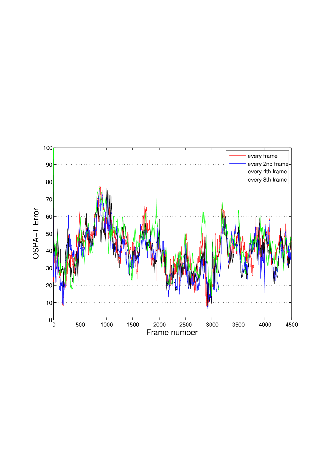
Figure 3: The influence of detection frequency on Algorithm 3: OSPA-T error for the sequence of $4500$ frames; OSPA-T metric parameters: $p=p^{\prime}=1$, $c=100$ and $\alpha=75$.

Head and body detection algorithms are very computationally intensive and consequently in real-time applications it may not be possible to provide them at every image frame. Next we compare the OSPA-T error performance of Algorithm 3 for the situations where head and body detections are available for: (1) every frame, (2) every 2nd frame, (3) every 4th frame and (4) every 8th frame. The results are shown in Fig.3. We note that the error performance does not change dramatically with the reduced frequency of head and body detections. The time averaged OSPA-T error for the four cases are: 40.7, 37.9, 39.2, and 42.7. Somewhat surprisingly, using body/head detections every 2nd and every 4th frame, reduces the number of false tracks and overall improves the accuracy. Only when body/head detections become available only every 8th frame, some of the true tracks start to be missing occasionally and consequently the OSPA-T error performance deteriorates.

V Conclusions

The paper presented a framework for performance evaluation of multi-object trackers. The framework is illustrated in the context of video tracking by comparison of three random-set based pedestrian tracking algorithms, using a video data set of a busy town centre. The multi-object tracking error was evaluated using the “OSPA for tracks” (OSPA-T) metric. The OSPA-T metric has an important property that it satisfies the axioms of a metric. The mathematical proof the triangle inequality axiom is presented in the paper.

The results of performance evaluation indicate that the CPHD based tracker of [13] performs the best. Although this is a single-frame recursive algorithm, its performance is comparable to that of [10] (which operates over a sliding window of frames). Future work will consider a smoothing version of the algorithm in [13] since a delay by a few frames in reporting the tracks is tolerable and has the potential to further improve the tracking accuracy.

References

- [1] R. Mahler, Statistical Multisource Multitarget Information Fusion. Artech House, 2007.
- [2] R. P. S. Mahler, “Multi-target Bayes filtering via first-order multi-target moments,” IEEE Trans. Aerospace & Electronic Systems, vol. 39, no. 4, pp. 1152–1178, 2003.
- [3] ——, “PHD filters of higher order in target number,” IEEE Trans. Aerospace & Electronic Systems, vol. 43, no. 4, pp. 1523–1543, 2007.
- [4] B.-T. Vo, B. Vo, and A. Cantoni, “The cardinality balanced multi-target multi-Bernoulli filter and its implementations,” IEEE Trans. Signal Processing, vol. 57, no. 2, pp. 409–423, 2009.
- [5] D. Clark, I. T. Ruiz, Y. Petillot, and J. Bell, “Particle PHD filter multiple target tracking in sonar image,” IEEE Trans. Aerospace & Electronic Systems, vol. 43, no. 1, pp. 409–416, 2007.
- [6] N. T. Pham, W. Huang, and S. H. Ong, “Tracking multiple objects using Probability Hypothesis Density filter and color measurements,” in Proc. IEEE Int. Conf. Multimedia and Expo, July 2007, pp. 1511 – 1514.
- [7] E. Maggio, M. Taj, and A. Cavallaro, “Efficient multitarget visual tracking using random finite sets,” IEEE Trans. Circuits & Systems for Video Technology, vol. 18, no. 8, pp. 1016–1027, 2008.
- [8] J. Sherrah, B. Ristic, and N. Redding, “Particle filter to track multiple people for visual surveillance,” IET Computer Vision, vol. 5, no. 4, pp. 192–200, 2011.
- [9] M. D. Breitenstein, F. Reichlin, B. Leibe, E. Koller-Meier, and L. V. Gool, “Robust tracking-by-detection using a detector confidence particle filter,” in Proc. IEEE Int. Conf. Computer Vision (ICCV), 2009.
- [10] B. Benfold and I. D. Reid, “Stable multi-target tracking in real-time surveillance video,” in Proc Computer Vision and Pattern Recognition (CVPR), 2011.
- [11] N. Dalal and B. Triggs, “Histograms of oriented gradients for human detection,” in Proc. IEEE Conf. Computer Vision and Pattern Recognition (CVPR), 2005.
- [12] A. Gning, B. Ristic, and L. Mihaylova, “Bernoulli particle/box-particle filters for detection and tracking in the presence of triple measurement uncertainty,” IEEE Trans. Signal Processing, 2012, (In print).
- [13] Y. Petetin, D. Clark, B. Ristic, and D. Maltese, “A tracker based on a CPHD filter approach for infrared applications,” in Proc. SPIE, 2011, vol. 8050.
- [14] B. E. Fridling and O. E. Drummond, “Performance evlauation methods for multiple target tracking algorithms,” in Proc. SPIE, Signal and Data Processing of Small Targets, vol. 1481, 1991, pp. 371–383.
- [15] S. B. Colegrove, L. M. Davis, and S. J. Davey, “Performance assessment of tracking systems,” in Proc. Intern. Symp. Signal Proc. and Applic. (ISSPA), Gold Coast, Australia, Aug. 1996, pp. 188–191.
- [16] G. Pingali and J. Segen., “Performance evaluation of people tracking systems,” in Proc. IEEE Workshop on Applications of Computer Vision, 1996.
- [17] T. Ellis, “Performance metrics and methods for tracking in surveillance,” in IEEE workshop on Performance Evaluation of Tracking and Surveillance, Copenhagen, Denmark, 2002.
- [18] F. Bashir and F. Porikli, “Performance evaluation of object detection and tracking systems,” in Proc. IEEE Int. Workshop Performance Evaluation of Tracking and Surveillance, 2006.
- [19] K. Bernardin and R. Stiefelhagen, “Evaluating multiple object tracking performance: The CLEAR MOT metrics,” Hindawi EURASIP Journal on Image and Video Processing, 2008.
- [20] B. Ristic, B.-N. Vo, D. Clark, and B.-T. Vo, “A metric for performance evaluation of multi-target tracking algorithms,” IEEE Trans. Signal Processing, vol. 59, no. 7, pp. 3452–3457, 2011.
- [21] D. Schuhmacher, B.-T. Vo, and B.-N. Vo, “A consistent metric for performance evaluation of multi-object filters,” IEEE Trans. Signal Processing, vol. 56, no. 8, pp. 3447–3457, Aug. 2008.
- [22] U. o. O. Active Vision Group, Dept. Engineering Science, “Town centre dataset,” http://www.robots.ox.ac.uk/ActiveVision/Research /Projects/2009bbenfold_headpose/project.html#datasets, Accessed Dec. 2011.
- [23] V. Prisacariu and I. Reid, “fastHOG – a real-time GPU implementation of HOG,” University of Oxford, Tech. Rep., 2009.
- [24] S. Blackman and R. Popoli, Design and Analysis of Modern Tracking Systems. Artech House, 1999.
- [25] J. E. L. G. H. Hardy and G. Pólya, Inequalities. Cambridge University Press, 1934.
- [26] B.-T. Vo, C.-M. See, N. Ma, and W.-T. Ng, “Multi-sensor joint detection and tracking with the Bernoulli filter,” IEEE Trans. Aerospace and Electronic Systems, 2012, (In print).
- [27] D. Musicki and B. L. Scala, “Multi-target tracking in clutter without measurement assignment,” IEEE Trans. Aerospace and Electronic Systems, vol. 44, no. 3, pp. 877–896, July 2008.
- [28] B. Ristic, B.-N. Vo, and D. Clark, “Performance evaluation of multi-target tracking using the OSPA metric,” in Proc. 13th Int. Conf. Information Fusion. Edinburgh, UK: ISIF, July 2010.
- [29] R. Mahler, “The multisensor PHD filter I: General solution via multitarget calculus,” in Proc. SPIE, vol. 7336, 2009.