Modelling grand minima of solar activity using a flux transport dynamo model

Abstract

The occurrence of grand minima like the Maunder minimum is an intriguing aspect of the sunspot cycle. We use the flux transport dynamo model to explain the grand minima, showing that they arise when either the poloidal field or the meridional circulation falls to a sufficiently low value due to fluctuations. Assuming these fluctuations to be Gaussian and determining the various parameters from the data of the last 28 cycles, we carry on a dynamo simulation with both these fluctuations. The results are remarkably close to the observational data.

1 Introduction

Early observations of sunspots revealed that there was an epoch from 1645 to 1715 when sunspots almost disappeared from the surface of the Sun. This period is known as the Maunder minimum. This was not an artifact of very few observations as this period was well covered by direct observations (Hoyt & Schatten 1996). Several old archival data have shown that there was a strong north-south asymmetry during the last phase of the Maunder minimum because most of the sunspots appeared in the southern hemisphere of the Sun (Ribes & Nesme-Ribes 1993). From the study of cosmogenic isotopes ¹⁰Be and ¹⁴C, it was found that the solar activity was weaker during the Maunder minimum, but the cyclic oscillation of solar activity continued with periods longer than the usual 11 years (Miyahara et al. 2004). The production of these isotopes varies with the solar cycle because the strong magnetic field of the Sun during solar maximum suppresses the Earth-ward incoming cosmic rays flux. The study of cosmogenic isotopes revealed that the Maunder minimum, which has been seen in the direct observational data during the seventeenth century, was not unique (Usoskin, Solanki & Kovaltsov 2007; Nagaya et al. 2012). In particular, from the study of ¹⁴C data, Usoskin, Solanki & Kovaltsov (2007) reported that there have been about 27 grand minima in the last 11,000 years and the Sun spent about 17% of this time in the grand minima state.

Our motivation is to study the physics behind the origin of these grand minima and then to find out their frequency using a dynamo model. Our calculations are based on the flux transport dynamo model, which is the most promising model at present to study the solar cycle and of which a version has been developed in our group over the years (Choudhuri, Schüssler & Dikpati 1995; Nandy & Choudhuri 2002; Chatterjee, Nandy & Choudhuri 2004; Chatterjee & Choudhuri 2006; Goel & Choudhuri 2009; Karak & Choudhuri 2012; Karak & Petrovay 2013; Karak & Nandy 2012). The details of this model have been reviewed by Choudhuri (2011). Basically this is a kinematic mean-field dynamo model in which the strong toroidal field is generated near the base of the convection zone by the differential rotation and the poloidal field is generated from the decay of the tilted bipolar sunspots near the solar surface (Babcock-Leighton process). The meridional circulation and the turbulent diffusivity provide the two important transport processes in this model for transporting the poloidal field from the top of the convection zone to the bottom.

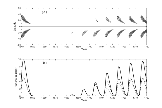
Figure 1: Theoretical Maunder minimum produced by making the poloidal field weak. (a) The butterfly diagram. (b) The smoothed sunspot number. The dashed and dotted lines show the sunspot numbers in southern and northern hemispheres, whereas the solid line is the total sunspot number. From Choudhuri & Karak (2009).

2 Modelling the Maunder minimum

Let us begin by looking at the possible sources of fluctuations in the flux transport dynamo model which can produce grand minima. A detailed discussion of our present understanding of the mechanisms that may cause grand minima has been reviewed by Choudhuri (2012). Therefore we are not going into the same discussion again. We believe that the possible mechanisms for producing the grand minima are the following: i) fluctuations in the Babcock-Leighton (B-L) process that may make the poloidal field weak and ii) fluctuations in the meridional circulation that may make it slow.

Let us look at the B-L process first. In this process, the poloidal field is generated from the decay of the tilted bipolar sunspots. This is a complex nonlinear process which depends on many factors, such as tilt angles of the bipolar sunspots. It has been found that the average tilt angle varies cycle to cycle making the poloidal field different at every solar minimum from its mean value (Dasi-Espuig et al. 2010). While the tilts of bipolar sunspots are produced by the Coriolis force acting on the rising toroidal flux tubes (D’Silva & Choudhuri 1993), the fluctuations in the tilts presumably result from the buffeting of the flux tubes by turbulence (Longcope & Choudhuri 2002). These fluctuations in tilts introduce fluctuations in the B-L process that has been identified as a main source of irregularities in solar cycles (Choudhuri, Chatterjee & Jiang 2007; Jiang, Chatterjee & Choudhuri 2007). Several authors (Choudhuri 1992; Charbonneau, Blais-Laurier & St-Jean 2004, Passos & Lopes 2011) introduced fluctuations in the poloidal field generation process and found intermittencies resembling grand minima. We model the Maunder minimum with the assumption that the poloidal field before the Maunder minimum dropped to a very low value. All our studies are based on the flux transport dynamo model presented by Chatterjee, Nandy & Choudhuri (2004), with a few parameters modified by Karak (2010). To produce the Maunder minimum, we (Choudhuri & Karak 2009) did the following. We stop the code at a solar minimum and change the poloidal field by a factor $\gamma$. We take $\gamma=0.4$ in southern hemisphere and $0.0$ in northern hemisphere. After this modification in the poloidal field, we again run the model for several solar cycles. Figure 1 shows the result of this procedure. Note that for the sake of comparison with the observation data, we have marked the beginning of this figure to be the year 1640. Our results successfully reproduce the north-south asymmetry in the sunspots and the sudden initiation of Maunder minimum and the gradual recovery.

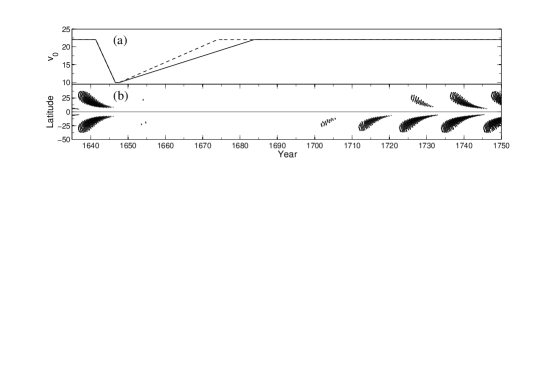
Figure 2: (a) The solid and dashed lines show the variations of $v_{0}$ (in m s^-1) in northern and southern hemispheres with time. (b) Butterfly diagram during the Maunder minimum. From Karak (2010).

The other important source of fluctuations in this dynamo model is the variations of the meridional circulation. There is no long-term observational data of the meridional circulation in the past. Therefore we do not directly know whether the meridional circulation had large variations with time. However, we know that there have been variations in the periods of solar cycles. Since the period of the flux transport dynamo strongly depends on the strength of the meridional circulation (Yeates, Nandy & Mackey 2008), we believe that the variations in the periods of the past cycles imply variations in the meridional circulation. Karak & Choudhuri (2011) used this idea to get a rough idea about the variations of meridional circulation. They also showed that such temporal variations in the meridional circulation are necessary to model the Waldmeier effect. To produce the Maunder minimum, Karak (2010) decreased the amplitude of meridional circulation rapidly to a very low value during a cycle and then, after a few years, it was increased to the usual value. By doing this, he is able to reproduce the Maunder minimum remarkably well. Figure 2 shows this result. The physics of this result can be understood from Yeates, Nandy & Mackey (2008) in the following way. When we decrease the meridional circulation to a very low value, the solar cycle periods become longer and the poloidal field remains in the convection zone for longer time. There are two competing effects – i) the differential rotation gets more time to induct the toroidal field which makes the toroidal field stronger and ii) diffusion gets more time to diffuse the fields which makes the toroidal field weaker. Now, in our high diffusivity model, the latter effect (the diffusion of the fields) is more important. A sufficiently weak meridional circulation can make the toroidal field so weak that the dynamo is pushed into a grand minimum state.

3 Estimating the probability of grand minima

In the observation data of last 11,000 yrs, there were 27 grand minima with durations longer than about 20 yrs. Therefore the probability that a particular solar cycle triggers a grand minimum is $2.7\%$. Our present motivation is to see whether the existing flux transport dynamo model can give a correct value of this probability. In the previous section, we have seen that the Maunder minimum can be reproduced either by decreasing the poloidal field to a very low value or by decreasing the meridional circulation to a very low value. However, instead of reducing either of these two quantities to a very low value, if we reduce both simultaneously, then we can reproduce the Maunder minimum for more moderate values of these two quantities. Karak (2010) gave the required values of the strength of the meridional circulation $v_{0}$ and the strength of the poloidal field $\gamma$ which can produce a Maunder-like grand minimum (see Fig. 6 of Karak 2010). Here we present a similar plot in Fig. 3. Parameters lying on the solid line produce grand minima of duration about 20 yrs. If the parameters lie below the solid line, then we get grand minima of durations more than 20 yrs. The shaded region in Fig. 3 should, therefore, cover all the grand minima observed in the past. Now the question is how to find out the values of these $v_{0}$ and $\gamma$ in the past. Obviously there is no direct way to find out these values. We (Choudhuri & Karak 2012) got these values in indirect ways. We find the values of $v_{0}$ by assuming that $v_{0}$ goes inversely as the solar cycle period. Therefore, from the observed periods of the last 28 solar cycles, we get 28 data for the $v_{0}$ and construct the histogram shown in Fig. 4(a). The Gaussian fit to this histogram is shown by the solid line in Fig. 4(a). Next we find out the values of the poloidal field by assuming a perfect correlation between the peak sunspot number and the poloidal field strength of the previous cycle. Therefore we again get 28 data points for $\gamma$ from the peak sunspot numbers of last 28 solar cycles. The histogram is shown in Fig. 4(b), with a Gaussian fit. The joint probability density that $v_{0}$ and $\gamma$ of a cycle lie in the range $v_{0}$, $v_{0}+$d$v_{0}$ and $\gamma$, $\gamma+$d$\gamma$ is given by

$$P(\gamma,v_{0})d\gamma dv_{0}=\frac{1}{\sigma_{v}\sqrt{2\pi}}\exp\left[-\frac{(v_{0}-\overline{v_{0}})^{2}}{2\sigma_{v}^{2}}\right]\times\frac{1}{\sigma_{\gamma}\sqrt{2\pi}}\exp\left[-\frac{(\gamma-1)^{2}}{2\sigma_{\gamma}^{2}}\right]d\gamma\,dv_{0}.$$

By integrating the above probability density over the shaded region in Fig. 3, we get the probability of a solar cycle triggering a grand minimum as $1.3\%$, which is not very far from the observed value $2.7\%$.

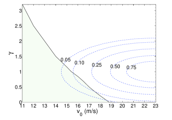
Figure 3: The solid line shows the values of the meridional circulation amplitude $v_{0}$ and the poloidal field scale factor $\gamma$ which produce grand minima of duration $\sim 20$ yrs. The parameters lying in the shaded region produce grand minima of longer duration. The dashed curves are the contours of the joint probability $P(\gamma,v_{0})$, with the values of $P(\gamma,v_{0})$ (excluding the constant pre-factor) given in the plot. From Choudhuri & Karak (2012).

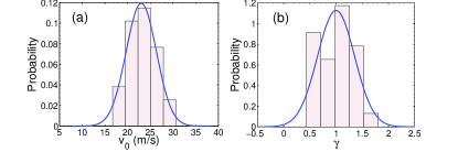
Figure 4: Histograms of the derived strength of (a) the meridional circulation $v_{0}$ and (b) the poloidal fieldṪhe solid curves are the Gaussian functions with means and standard deviations 23 m s^-1 3.34 m s^-1 in (a) and 1 and $0.35$ in (b). From Choudhuri & Karak (2012).

4 Simulations of grand minima

To check whether the above simple argument about the occurrence probability of grand minima is borne out by detailed calculations, we (Choudhuri & Karak 2012; Karak & Choudhuri 2013) have carried out extensive simulations with our dynamo model. We introduce stochastic fluctuations both in the poloidal field and the meridional circulation. To introduce fluctuations in the poloidal field, we change the poloidal field by the factor $\gamma$ above $0.8R_{\odot}$ at every solar minima (for details see Choudhuri, Chatterjee & Jiang 2007), whereas to introduce fluctuations in the meridional circulation, we change $v_{0}$ everywhere in the model after a certain coherence time of 30 yrs. We choose the fluctuation levels of the poloidal field and the meridional circulation according to their distributions shown in Fig. 4. A result of a typical run of 11,000 yrs is shown in Fig. 5. In this particular run, we get 28 grand minima. We have carried out several simulations with different realizations of the random numbers for the poloidal field and the meridional circulation, finding that the numbers of grand minima in all simulations lie in the range 24-30 remarkably close to the observed number 27. Another important result we find is that the Sun spent about 10–15% of the total time in grand minima state which is close to the observed value 17%. We have also checked how the results change with the coherence time of meridional circulation by performing several simulations with varying coherence time. We have seen that when we take the coherence time less than about 15 yrs, the number of grand minima becomes considerably less.

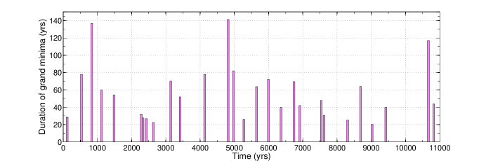
Figure 5: The durations of grand minima indicated by vertical bars at their times of occurrence in a 11,000 yr simulation. This is the result of a particular realization of random fluctuations that produced 28 grand minima. From Choudhuri & Karak (2012).

One important point to note is that the B-L process may not work during grand minima, since very few sunspots appear during those times. Therefore the question remains unclear how the Sun recovers from a grand minimum after entering one. We believe that the turbulent $\alpha$ effect originally proposed by Parker (1955) might be a good candidate for generating a weak poloidal field and this could eventually pull the Sun out of the grand minimum. Since the detailed nature of this $\alpha$ effect is unclear, our first calculations described here use the same B-L $\alpha$ all the time. However our future work (Karak & Choudhuri 2013) explores this issue.

5 Conclusion

We have explored the possible causes of the grand minima using a flux transport dynamo model. We believe that the fluctuations in the poloidal field and in the meridional circulation are the two important sources of randomness in this dynamo model. We have shown that a weak poloidal field or a weak meridional circulation or both can push the Sun into a grand minimum. We have also studied the frequency of occurrence of the grand minima. We have derived the levels of the fluctuations of the poloidal field and the meridional circulation from the data of last 28 solar cycles. Then we use these observationally derived fluctuations in our dynamo model to simulate grand minima in a run of 11,000 yrs. Our result of the frequency of the grand minima is exceptionally close to the observational result. The details of this work, including the recovery mechanism of grand minima, and the grand maxima can be found in recent work (Karak & Choudhuri 2013).