Cepheids and other short-period variables near the Galactic Centre

Abstract

We report the result of our near-infrared survey of short-period variable stars ($P<60$ d) in a field-of-view of $20^{\prime}\times 30^{\prime}$ towards the Galactic Centre. Forty-five variables are discovered and we classify the variables based on their light curve shapes and other evidence. In addition to 3 classical Cepheids reported previously, we find 16 type II Cepheids, 24 eclipsing binaries, one pulsating star with $P=0.265$ d (RR Lyr or $\delta$ Sct) and one Cepheid-like variable whose nature is uncertain. Eclipsing binaries are separated into the foreground objects and those significantly obscured by interstellar extinction. One of the reddened binaries contains an O-type supergiant and its light curve indicates an eccentric orbit. We discuss the nature and distribution of type II Cepheids as well as the distance to the Galactic Centre based on these Cepheids and other distance indicators. The estimates of $R_{0}$(GC) we obtained based on photometric data agree with previous results obtained with kinematics of objects around the GC. Furthermore, our result gives a support to the reddening law obtained by Nishiyama and collaborators, $A_{K_{\mathrm{s}}}/E(H-K_{\mathrm{s}})=1.44$, because a different reddening law would result in a rather different distance estimate.

1 Introduction

The Galactic Centre (hereafter GC) region is an important place for many reasons. A supermassive black hole exists in the direction of Sgr A^∗ within a complex region involving both hot and cold gas (e.g. Morris & Serabyn 1996; Genzel, Eisenhauer & Gillessen, 2010). This region hosts the highest density of stars in the Galaxy, and furthermore various stellar populations co-exist with different distribution and characteristics (Launhardt, Zylka & Mezger, 2002). First, the extended Bulge with a scale of a few kilo-parsecs has a triaxial or bar-like shape (Nakada et al. 1991; Whitelock & Catchpole 1992; Stanek et al. 1994) and is populated predominantly by old stars ($\geq 10$ Gyr, Zoccali et al. 2003; Clarkson et al. 2011). Secondly, the nuclear bulge show a disk-like distribution with a radius $\sim 200$ parsecs, and a significant population of young stars (a few Myr) are found in this region (Serabyn & Morris 1996; Figer et al. 2004; Yusef-Zadeh et al. 2009). Finally, a dense stellar cluster with numerous massive stars exist within a radius $\sim 10$ parsecs (its core radius actually is much smaller, $\sim 0.3$ parsec) around the central black hole (Genzel et al., 2003). The GC region provides us with a unique opportunity to study not only stellar evolution but also phenomena in central parts of galaxies at close hand ($\sim 8$ kpc). For instance, the most populous group of known young and massive stars, such as O-type stars and Wolf-Rayet stars, within the Galaxy exists there (e.g. Mauerhan et al. 2010).

Pulsating variable stars are useful in studies of stellar populations. In particular, Cepheids play important roles in a wide range of astronomy. There are two groups of Cepheids, i.e. classical Cepheids (hereafter CCEPs) and type II Cepheids (T2Cs). Both of them have period-luminosity relation (PLR), but the luminosities at a given period differ by 1.5–2 mag (Sandage & Tammann 2006; Matsunaga, Feast & Soszyński, 2011a). CCEPs are pulsating supergiants with periods typically between 3 and 50 d, evolved from intermediate- to high-mass stars (4–10 $M_{\odot}$). On the other hand, T2Cs have similar periods to CCEPs, but are old and evolved from low-mass stars, $\sim 1~{}M_{\odot}$. T2Cs are conventionally subdivided into the BL Her and W Vir stars at periods less than 20 days and the RV Tau stars with greater periods. In addition, Soszyński et al. (2008b) identified peculiar W Vir stars which tend to be brighter than the PLR and to often show light curves with eclipsing or ellipsoidal modulation. There remain uncertainties in the properties and the evolution of T2Cs (see the discussion in Matsunaga et al. 2011a).

A serious difficulty in studying the stars towards the GC lies in observing them beyond the severe interstellar extinction. The foreground extinction is not uniform and strong (around 2–3 mag in the $K$ band, $2.2~{}\mu{\mathrm{m}}$). Thus, infrared observations are required in order to study stars in the GC region. In fact long-term infrared observations have made it possible to monitor stellar motions around the central black hole (Ghez et al. 2008; Gillessen et al. 2009, and references therein). These and other data were used to search for variable stars in the few parsec (or smaller) region around Sgr A^∗ (Tamura et al. 1996; Ott, Eckart & Genzel, 1999; Peeples, Stanek & DePoy, 2007; Rafelski et al. 2007). However, no Cepheids were found in these works.

We carried out near-IR observations to investigate stellar variability in the GC region. Our survey covered a much wider area, $20^{\prime}\times 30^{\prime}$, than the previous monitoring observations. A large number of long-period variables including Miras were found in the survey region (Matsunaga et al. 2009b, =Paper I), and we discovered three CCEPs, the first of this type in the GC region (Matsunaga et al. 2011b, =Paper II). In the present paper we describe our data analysis and a catalogue of the short period variables in the field, and also discuss their nature as well as the distance to the GC.

2 Observation and data reduction

Observations were conducted using the IRSF 1.4 m telescope and the SIRIUS camera (Nagashima et al. 1999; Nagayama et al. 2003) which collects images in the $J~{}(1.25~{}\mu\mathrm{m})$, $H~{}(1.63~{}\mu\mathrm{m})$ and $K_{\mathrm{s}}~{}(2.14~{}\mu\mathrm{m})$ bands, simultaneously. The observed field composed of 12 fields-of-view of IRSF/SIRIUS covered $20^{\prime}\times 30^{\prime}$ around the GC (Table 1). Observations at about 90 epochs were made between 2001 and 2008 of which the majority were obtained in 2005 and 2006. We used this dataset in Paper I and II, and further observational details are found there.

Table 1: The observed fields. The central coordinates, the numbers of monitorings and the numbers of short-period variables are listed.

Field	RA (J2000)	Dec. (J2000.0)	$N_{\mathrm{obs}}$	$N_{\mathrm{Short}}$
1745$-$2900A	17:46:10.5	$-$28:53:47.8	94	3
1745$-$2900B	17:45:40.0	$-$28:53:47.8	92	6
1745$-$2900C	17:45:09.5	$-$28:53:47.8	90	3
1745$-$2900D	17:46:10.5	$-$29:00:28.0	93	3
1745$-$2900E	17:45:40.0	$-$29:00:28.0	91	6†
1745$-$2900F	17:45:09.5	$-$29:00:28.0	89	5†
1745$-$2900G	17:46:10.5	$-$29:07:07.8	87	4
1745$-$2900H	17:45:40.0	$-$29:07:07.8	89	3
1745$-$2900I	17:45:09.5	$-$29:07:07.8	83	4
1745$-$2840G	17:46:10.5	$-$28:47:07.9	85	6
1745$-$2840H	17:45:40.0	$-$28:47:07.9	85	1
1745$-$2840I	17:45:09.5	$-$28:47:07.9	60	2
Total				45‡

^† One object, #15 in Table 2, was detected in the overlapping region of both fields. ^‡ We do not include the duplicate detection in the neighbouring fields.

The basic data analysis was done in the same manner as in Paper I. In short, point-spread-function (PSF) fitting photometry was performed on every images using the IRAF/DAOPHOT package, and variable stars were searched for by combining the time-series sets of $JHK_{\rm s}$ magnitudes. The standard deviations (SDs) were calculated for repeated measurements of individual stars. We then looked for variable stars with SD more than three times larger than the median value of SDs in the corresponding magnitude range. The variability search was done using the three band datasets independently, so that we could find variables even if they are visible only in one of the $JHK_{\rm s}$ bands.

The saturation limits are 9.5, 9.5 and 9.0 mag, and the detection limits are around 16.4, 14.5 and 13.1 mag in $J$, $H$ and $K_{\mathrm{s}}$, respectively. The definition of these values is described in Paper I, but the detection limits vary across the survey region depending on the crowdedness. Especially, the central region around Sgr A^∗ is so crowded that the accuracy of our photometric measurements, with the typical seeing of $\sim 1^{\prime\prime}$, is rather limited. The detection limit also changes from frame to frame depending on the weather condition. Therefore, the above limiting magnitudes should be considered only as typical values.

While we catalogued 1364 long-period variables in Paper I, variables with period shorter than 60 days are presented in this paper. Periods $P$ were determined by fitting the following fourth-order Fourier series,

$$m(t)=A_{0}+\sum_{i=1}^{4}A_{i}\cos(2\pi it/P+\phi_{i}).$$ (1)

The light curves of Cepheids, which are our main targets, are known to be fitted by such Fourier series well (e.g. Laney & Stobie 1993).

3 Results

3.1 Detection of short-period variables

Table 2: The catalogue of short-period variables detected towards the Galactic Centre. After the numbering ID between #1 and #45, the ID combining RA and Dec. (J2000.0) follows. Then listed are galactic coordinates, $JHK_{\rm s}$ mean magnitudes, peak-to-valley amplitudes, $M$flag (see the text) and periods. The classifications are also indicated as: Cep(I)$=$classical Cepheid, Cep(II)$=$type II Cepheid, Ecl$=$eclipsing binary (see also Table 5). #3 may be either of an RR Lyr or a $\delta$ Sct star. #34 seems to be a kind of Cepheid, possibly an anomalous Cepheid, but it is unclear which group it belongs to. For eclipsing binaries except #30, half the orbital periods are listed.

No.	ID	$l$	$b$	$J$	$H$	$K_{\mathrm{s}}$	$\Delta J$	$\Delta H$	$\Delta K_{\mathrm{s}}$	Mflag	Period	Type
		($\circ$)	($\circ$)	(mag)	(mag)	(mag)	(mag)	(mag)	(mag)		(d)
1	17445710$-$2910057	$-0.2742$	$+0.0036$	15.55	14.35	—	0.56	0.52	—	003	0.3613	Ecl
2	17445906$-$2851235	$-0.0046$	$+0.1602$	15.57	14.08	12.73	1.22	1.03	0.62	777	7.46	Cep(II)
3	17445910$-$2909440	$-0.2652$	$+0.0005$	13.76	12.53	11.72	0.23	0.13	0.31	000	0.265	RR/DS
4	17450132$-$2848213	$+0.0428$	$+0.1796$	—	14.46	12.87	—	0.71	0.69	300	12.544	Ecl
5	17450204$-$2857215	$-0.0838$	$+0.0990$	14.58	14.06	—	0.66	0.56	—	003	0.17733	Ecl
6	17450754$-$2906573	$-0.2097$	$-0.0015$	—	14.13	12.51	—	0.61	0.68	300	15.097	Cep(II)
7	17450913$-$2859417	$-0.1035$	$+0.0567$	16.37	13.02	11.33	0.68	0.47	0.40	000	52.224	Cep(II)
8	17451032$-$2904526	$-0.1749$	$+0.0079$	14.08	13.39	12.42	0.35	0.44	0.35	077	0.21968	Ecl
9	17451383$-$2844443	$+0.1181$	$+0.1721$	—	15.19	13.69	—	0.53	0.50	300	4.747	Cep(II)
10	17451719$-$2857531	$-0.0624$	$+0.0474$	—	14.49	12.47	—	0.74	0.86	300	24.09	Cep(II)
11	17451764$-$2851372	$+0.0275$	$+0.1004$	—	14.91	13.30	—	0.34	0.35	300	8.2713	Cep(II)
12	17452092$-$2858186	$-0.0614$	$+0.0321$	14.30	13.53	—	0.87	0.77	—	003	0.15869	Ecl
13	17452219$-$2853583	$+0.0027$	$+0.0658$	12.58	12.29	12.11	0.34	0.34	0.33	000	1.6094	Ecl
14	17452573$-$2909397	$-0.2137$	$-0.0815$	—	14.37	12.76	—	0.43	0.41	377	1.0984	Ecl
15	17452600$-$2900037	$-0.0766$	$+0.0010$	15.69	12.93	11.36	0.90	0.92	0.96	000	50.46	Cep(II)
16	17452837$-$2858221	$-0.0480$	$+0.0084$	15.02	13.94	—	0.54	0.52	—	003	1.5838	Ecl
17	17452987$-$2854290	$+0.0101$	$+0.0375$	14.97	12.18	10.67	0.29	0.26	0.27	000	1.6448	Ecl
18	17453089$-$2903105	$-0.1116$	$-0.0412$	16.36	12.44	10.35	0.68	0.44	0.51	000	22.76	Cep(I)
19	17453148$-$2859531	$-0.0637$	$-0.0145$	10.98	10.84	10.70	0.10	0.10	0.18	000	3.6301	Cep(II)
20	17453227$-$2902552	$-0.1054$	$-0.0433$	15.42	12.00	10.17	0.60	0.46	0.57	000	19.96	Cep(I)
21	17454075$-$2852367	$+0.0574$	$+0.0198$	—	14.93	13.31	—	0.39	0.47	300	0.55648	Ecl
22	17454904$-$2856450	$+0.0142$	$-0.0419$	13.81	13.40	13.02	0.55	0.62	0.71	007	0.41278	Ecl
23	17455015$-$2855069	$+0.0396$	$-0.0312$	—	14.25	12.53	—	0.36	0.42	377	1.628	Ecl
24	17455150$-$2903392	$-0.0793$	$-0.1094$	14.18	13.72	13.58	0.40	0.42	0.54	000	0.24946	Ecl
25	17455257$-$2900004	$-0.0254$	$-0.0811$	17.05	14.03	12.19	0.89	0.57	0.58	700	1.7092	Ecl
26	17455318$-$2856206	$+0.0279$	$-0.0512$	—	14.28	12.40	—	0.84	0.85	000	16.1	Cep(II)
27	17455325$-$2904069	$-0.0826$	$-0.1189$	—	14.53	12.89	—	0.41	0.42	300	1.7316	Ecl
28	17455413$-$2845032	$+0.1904$	$+0.0437$	—	14.62	12.95	—	0.77	0.73	300	15.543	Cep(II)
29	17455482$-$2854382	$+0.0553$	$-0.0415$	—	15.29	13.58	—	0.45	0.61	377	10.26	Cep(II)
30	17460164$-$2855155	$+0.0594$	$-0.0682$	13.40	10.64	9.16	0.40	0.42	0.32	000	26.792	Ecl
31	17460200$-$2852506	$+0.0944$	$-0.0484$	—	12.98	11.37	—	0.61	0.68	377	40.13	Cep(II)
32	17460601$-$2846551	$+0.1864$	$-0.0095$	15.63	12.04	10.18	0.58	0.45	0.44	000	23.538	Cep(I)
33	17460637$-$2909442	$-0.1377$	$-0.2084$	12.68	10.91	10.07	0.12	0.14	0.10	000	18.96	Cep(II)
34	17461000$-$2855325	$+0.0712$	$-0.0967$	15.01	12.28	10.79	0.21	0.17	0.19	077	2.1932	Cep(?)
35	17461007$-$2905173	$-0.0674$	$-0.1814$	16.10	—	—	0.73	—	—	033	0.14612	Ecl
36	17461044$-$2903183	$-0.0385$	$-0.1653$	12.43	11.89	11.18	0.79	0.72	0.56	077	0.97209	Ecl
37	17461171$-$2850001	$+0.1533$	$-0.0540$	16.08	13.45	11.91	0.74	0.56	0.60	000	0.94255	Ecl
38	17461252$-$2848526	$+0.1709$	$-0.0468$	—	14.24	12.24	—	0.59	0.54	300	1.6486	Ecl
39	17461356$-$2848351	$+0.1770$	$-0.0475$	—	—	12.75	—	—	0.86	337	31.17	Cep(II)
40	17461357$-$2859023	$+0.0282$	$-0.1381$	—	14.91	13.03	—	1.00	0.84	300	19.014	Cep(II)
41	17461447$-$2849002	$+0.1728$	$-0.0539$	13.80	12.57	10.98	0.73	0.53	0.27	077	0.14161	Ecl
42	17461626$-$2850125	$+0.1590$	$-0.0700$	15.63	12.97	11.39	0.77	0.70	0.72	000	1.66284	Ecl
43	17462426$-$2908288	$-0.0860$	$-0.2531$	—	14.06	12.49	—	0.60	0.69	300	13.52	Ecl
44	17462642$-$2857079	$+0.0797$	$-0.1616$	14.33	13.53	13.23	0.30	0.35	0.37	000	0.41546	Ecl
45	17462846$-$2908562	$-0.0846$	$-0.2702$	17.17	14.03	12.46	1.34	0.99	1.10	000	24.406	Cep(II)

We detected 45 variable stars with period between 0.14 and 52.1 d. The number of the objects found in each field-of-view is indicated in Table 1. Table 2 lists their IDs, galactic coordinates, mean magnitudes, amplitudes and periods. The mean magnitudes are intensity-scale means of maximum and minimum, and the amplitudes refer to peak-to-valley variations. The $JHK_{\rm s}$ time-series data obtained for all the catalogued variables are compiled in one text file and each line includes the ID number, the modified Julian date (MJD) and the $JHK_{\rm s}$ for each measurement. Table 3 shows the first 10 lines as a sample of the full version to be published online. Fig. 1 plots their folded light curves in the ascending order of period. Because the light curves of eclipsing variables are often nearly symmetrical, a fit of the Fourier series (eq. 1) tends to yield half the orbital period and this is listed in Table 2 except in the case of #30 whose light curve is significantly asymmetric. The orbital periods are used in Fig. 1.

We did not always detect the variables in all of the $JHK_{\rm s}$ bands. Table 2 includes $M$flag which we also used in Paper I to show the reasons of non-detection or the qualities of the listed magnitudes. In this work, only the flag numbers 0, 3 and 7 are relevant. The flags 0 and 3 respectively indicate that a mean magnitude was obtained properly and that some measurements were affected by the detection limit leading to an uncertain mean magnitude. The flag 7 is newly defined to indicate that the photometry of the object is affected by the crowding. None of our objects was too bright, and none was located too close to the edge of the detector. The light curves in Fig. 1 indicates that the entire variations from minima to maxima were sampled well enough to estimate mean magnitudes except for the faintest cases.

As we see in Fig. 1, our sample includes different types of variables. In order to determine the variable types, shapes of the light curves are discussed in Section 3.2. For CCEPs and T2Cs, as briefly discussed in Paper II, we also consider their absolute magnitudes and the expected distances (Section 3.3). In Section 3.4, we summarise the classification and compare some features among variable types.

Table 3: Light variations for the catalogued variables. When the magnitudes are not available we put 99.99 instead. This is the first 10 lines of the full catalogue (3707 lines), which will be available in the online version of the article (see Supporting Information).

No.	MJD	$J$	$H$	$K_{\mathrm{s}}$
1	52343.1514	15.60	14.49	99.99
1	53482.0694	15.28	14.22	99.99
1	53537.1167	15.57	99.99	99.99
1	53540.8287	15.69	14.56	99.99
1	53545.8959	15.67	14.49	99.99
1	53545.9758	15.32	14.24	99.99
1	53548.8325	15.48	99.99	99.99
1	53548.9662	15.32	14.20	99.99
1	53549.8964	15.53	14.39	99.99
1	53550.0148	15.32	14.17	99.99

Figure 1: Light curves of the catalogued variables plotted in the ascending order of period. For eclipsing variables, the orbital periods (twice the periods listed in Table 2) are used. The ID, the variable type and the (rounded) period are indicated at the top of each panel as well as the name of filter ($J$, $H$ or $K_{\mathrm{s}}$) used in the plot.

3.2 Shapes of the light curves

In order to give a quantitative description of the light curve shape, the parameters,

$$R_{21}=A_{2}/A_{1},$$ (2)

$$\phi_{21}=\phi_{2}-2\phi_{1},$$ (3)

$$R_{31}=A_{3}/A_{1},$$ (4)

$$\phi_{31}=\phi_{3}-3\phi_{1},$$ (5)

are considered for each light curve based on the fitted Fourier series (eq. 1). These parameters are listed in Table 4.

Table 4: The list of Fourier parameters for the observed light curves. Four parameters ($R_{21},\phi_{21},R_{31}$ and $\phi_{31}$, see eq. 2–5 for the definition) are listed for each of the $JHK_{\rm s}$ bands. The $\phi$ values are given in the unit of $\pi$.

No.	$\log P$	$J$-band				$H$-band				$K_{\mathrm{s}}$-band
		$R_{21}$	$\phi_{21}$	$R_{31}$	$\phi_{31}$	$R_{21}$	$\phi_{21}$	$R_{31}$	$\phi_{31}$	$R_{21}$	$\phi_{21}$	$R_{31}$	$\phi_{31}$
1	$-0.442^{\dagger}$	0.176	1.983	0.030	1.550	0.174	2.004	0.075	0.064	—	—	—	—
2	$0.873$	0.246	2.923	0.157	0.212	0.336	2.834	0.120	0.204	0.364	2.907	0.192	0.021
3	$-0.577$	0.312	1.181	0.181	0.690	0.309	1.304	0.242	0.862	0.526	1.484	0.144	1.518
4	$1.098^{\dagger}$	—	—	—	—	0.301	2.055	0.072	0.739	0.268	2.067	0.074	0.728
5	$-0.751^{\dagger}$	8.190	1.913	1.076	1.961	3.818	1.918	0.715	1.951	—	—	—	—
6	$1.179$	—	—	—	—	0.038	1.403	0.051	0.774	0.044	1.002	0.113	0.812
7	$1.718$	0.283	2.615	0.096	0.098	0.184	2.696	0.036	1.956	0.147	2.665	0.005	1.757
8	$-0.658^{\dagger}$	0.087	2.016	0.064	0.140	0.132	1.936	0.091	0.848	0.384	1.998	0.247	1.576
9	$0.676$	—	—	—	—	0.259	1.986	0.075	0.184	0.116	2.101	0.051	0.189
10	$1.382$	—	—	—	—	0.160	1.869	0.029	0.038	0.101	1.822	0.029	1.258
11	$0.918$	—	—	—	—	0.227	2.188	0.088	0.245	0.183	2.378	0.062	0.046
12	$-0.799^{\dagger}$	5.306	2.023	0.526	1.955	4.916	1.983	0.615	1.894	—	—	—	—
13	$0.207^{\dagger}$	0.683	1.912	0.568	1.877	0.733	1.923	0.585	1.888	0.689	1.949	0.621	1.932
14	$0.041^{\dagger}$	—	—	—	—	0.493	2.043	0.308	1.833	0.702	1.908	0.237	1.707
15	$1.703$	0.176	1.585	0.064	0.655	0.359	1.595	0.088	0.934	0.316	1.536	0.105	0.829
16	$0.200^{\dagger}$	0.946	2.063	0.934	0.072	0.856	2.036	0.819	0.043	—	—	—	—
17	$0.216^{\dagger}$	0.332	2.013	0.077	1.987	0.232	1.973	0.058	1.737	0.240	2.094	0.068	0.830
18	$1.357$	0.236	1.729	0.240	1.059	0.189	1.896	0.138	1.740	0.239	1.922	0.182	1.710
19	$0.560$	0.118	1.337	0.068	1.331	0.137	1.243	0.010	0.926	0.541	1.030	0.087	1.152
20	$1.300$	0.311	1.679	0.135	1.260	0.200	1.849	0.107	1.500	0.349	1.753	0.066	1.599
21	$-0.255^{\dagger}$	—	—	—	—	0.127	2.101	0.090	0.048	0.233	1.865	0.129	1.737
22	$-0.384^{\dagger}$	0.692	2.030	0.423	0.069	0.696	1.979	0.430	0.006	0.497	2.117	0.854	0.329
23	$0.212^{\dagger}$	—	—	—	—	1.853	2.542	0.189	0.838	1.713	2.694	0.114	1.046
24	$-0.603^{\dagger}$	0.161	2.003	0.025	1.545	0.189	2.013	0.015	0.797	0.253	2.023	0.051	0.319
25	$0.233^{\dagger}$	0.661	2.035	0.310	0.169	0.655	2.029	0.370	0.114	0.619	2.004	0.328	0.035
26	$1.207$	—	—	—	—	0.098	1.798	0.049	0.332	0.041	1.301	0.035	0.810
27	$0.238^{\dagger}$	—	—	—	—	0.586	2.064	0.513	0.210	0.805	2.118	0.620	0.233
28	$1.192$	—	—	—	—	0.015	1.944	0.056	0.673	0.067	1.129	0.040	0.874
29	$1.011$	—	—	—	—	0.108	2.278	0.041	0.511	0.093	1.753	0.185	0.738
30	$1.428$	1.969	1.022	0.856	1.179	1.818	1.016	0.734	1.160	1.656	2.980	0.566	1.157
31	$1.603$	—	—	—	—	0.151	1.749	0.049	0.952	0.118	1.719	0.084	0.843
32	$1.372$	0.299	1.671	0.189	1.422	0.253	1.879	0.129	1.698	0.210	1.910	0.101	1.735
33	$1.278$	0.036	2.932	0.055	1.459	0.034	1.853	0.121	1.310	0.085	1.345	0.109	1.236
34	$0.341$	0.124	1.771	0.180	1.735	0.086	1.757	0.029	0.409	0.049	1.722	0.068	1.395
35	$-0.835^{\dagger}$	0.318	2.076	0.148	0.093	—	—	—	—	—	—	—	—
36	$-0.012^{\dagger}$	0.458	1.978	0.265	1.985	0.461	1.985	0.252	0.003	0.414	1.935	0.234	1.949
37	$-0.026^{\dagger}$	0.155	2.014	0.100	0.186	0.166	1.991	0.094	1.960	0.128	1.902	0.135	1.912
38	$0.217^{\dagger}$	—	—	—	—	0.113	1.789	0.121	1.735	0.114	1.684	0.075	1.489
39	$1.494$	—	—	—	—	—	—	—	—	0.099	1.414	0.194	0.897
40	$1.279$	—	—	—	—	0.142	1.902	0.064	0.275	0.087	1.662	0.051	0.793
41	$-0.849^{\dagger}$	0.328	1.962	0.112	0.039	0.357	1.877	0.108	1.829	0.324	1.747	0.058	1.061
42	$0.221^{\dagger}$	0.324	1.999	0.152	1.978	0.362	1.970	0.175	0.008	0.348	1.946	0.158	0.002
43	$1.131^{\dagger}$	—	—	—	—	0.382	1.966	0.110	1.954	0.318	1.955	0.068	1.866
44	$-0.381^{\dagger}$	0.585	1.922	0.255	1.888	0.779	2.031	0.327	0.072	0.548	2.022	0.340	1.827
45	$1.387$	0.197	1.920	0.122	1.312	0.157	1.785	0.093	1.502	0.171	1.752	0.108	1.618

$\dagger$ Half the orbital periods are given for all the eclipsing binaries except #30.

We also consider the above Fourier parameters for the variables in the Large Magellanic Cloud (LMC), found in the Optical Gravitational Lensing Experiment (OGLE-III), to compare with our objects. In Fig. 2, different types of the LMC variables are plotted in different colours: CCEP (Soszyński et al., 2008a), T2Cs (Soszyński et al., 2008b), RR Lyr stars (Soszyński et al., 2009), and $\delta$ Sct stars (Poleski et al., 2010). Among the $\delta$ Sct reported by Poleski et al. (2010), single-mode stars without the uncertainty flag are used. Because they included only $R_{21}$ and $\phi_{21}$, we calculated $R_{31}$ and $\phi_{31}$ using their photometric data.

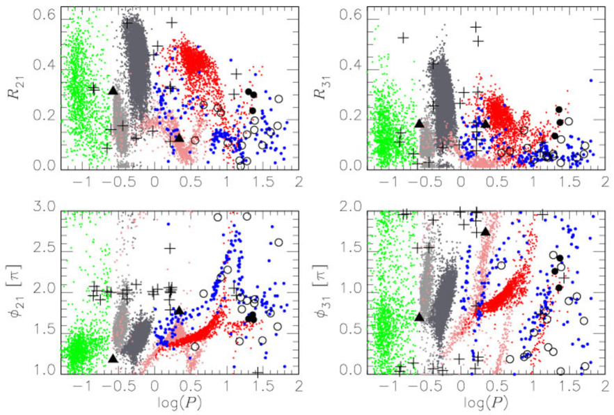
Figure 2: Fourier parameters (eq. 2–5) plotted against period. For eclipsing binaries except #30, half of the orbital periods are used. Black large symbols indicate our objects: filled circles for CCEPs, open circles for T2Cs, ’$+$’ symbols for binaries and triangles for others. The small dots indicate the OGLE-III variable stars of different types with different colours: red for CCEPs pulsating in the fundamental mode, pink for CCEPs in the overtone mode, blue for T2Cs in the fundamental mode, dark grey for RR Lyr stars in the fundamental mode, light grey for those in the overtone mode, and green for $\delta$ Sct stars. The Fourier parameters were obtained with the $I$-band light curves for the OGLE-III stars, while the light curve in the shortest wavelength available was used for each of our objects.

The OGLE-III light curves were taken in the $I$-band. The available light curves are rather limited in $JHK_{\rm s}$, but the result in Laney & Stobie (1993) suggests that, at least, $J$-band light curves are similar to the $I$-band ones for CCEPs. We plot the parameters for $J$-band light curves whenever possible for our objects. Those for $H$-band are used in other cases, but for the object with neither of $J$ and $H$ light curves the $K_{\mathrm{s}}$-band parameters are considered. The second column of Table 5 indicates the variability types judged by the light curve shapes.

Table 5: Classification of variable stars. The second column indicates the variable types whose light curve shapes are consistent with those of the objects. As the variable types, I and II stand for CCEPs and T2Cs, respectively, while Ecl stands for eclipsing binaries. The $A_{K_{\mathrm{s}}}$ and $D$ indicate approximate extinctions and distances for Cepheids (I$=$CCEPs, II$=$T2Cs). In the last column the concluded variable types are listed. See the details in the text where some comments on individual objects are also given.

No.	LC	$A_{K_{\mathrm{s}}}$	$D$	Type
	shape	(mag)	(kpc)
1	Ecl	—	—	Ecl
2	I/II:	1.3	23.9 (I), 9.0 (II)	Cep(II)
3	RR/DS	—	—	RR/DS $\dagger$
4	Ecl	—	—	Ecl
5	Ecl	—	—	Ecl
6	I/II:	2.1	22.2 (I), 6.9 (II)	Cep(II)
7	II	2.2	26.3 (I), 6.7 (II)	Cep(II)
8	Ecl	—	—	Ecl
9	II	1.9	19.1 (I), 7.7 (II)	Cep(II)
10	II	2.6	23.2 (I), 6.5 (II)	Cep(II)
11	II	2.1	21.6 (I), 7.7 (II)	Cep(II)
12	Ecl	—	—	Ecl
13	Ecl	—	—	Ecl
14	Ecl	—	—	Ecl
15	II	1.9	31.3 (I), 8.0 (II)	Cep(II)
16	Ecl	—	—	Ecl
17	Ecl	—	—	Ecl
18	I	2.7	7.7 (I), 2.3 (II)	Cep(I)
19	II:	0.0	9.9 (I), 4.3 (II)	Cep(II)
20	I	2.3	7.8 (I), 2.4 (II)	Cep(I)
21	Ecl	—	—	Ecl
22	Ecl	—	—	Ecl
23	Ecl	—	—	Ecl
24	Ecl:	—	—	Ecl
25	Ecl	—	—	Ecl
26	I/II:	2.4	18.7 (I), 5.7 (II)	Cep(II)
27	Ecl	—	—	Ecl
28	II	2.2	26.9 (I), 8.3 (II)	Cep(II)
29	I/II:	2.3	26.6 (I), 9.0 (II)	Cep(II)
30	Ecl	—	—	Ecl
31	II	2.1	25.4 (I), 6.4 (II)	Cep(II)
32	I	2.4	8.3 (I), 2.5 (II)	Cep(I)
33	II	1.1	13.0 (I), 4.1 (II)	Cep(II)
34	Cep:	1.9	3.0 (I), 1.4 (II)	Cep(?) $\dagger$
35	Ecl	—	—	Ecl
36	Ecl	—	—	Ecl
37	Ecl	—	—	Ecl
38	Ecl	—	—	Ecl
39	II	—	—	Cep(II)
40	II	2.4	28.0 (I), 8.3 (II)	Cep(II)
41	Ecl	—	—	Ecl
42	Ecl	—	—	Ecl
43	Ecl	—	—	Ecl
44	Ecl	—	—	Ecl
45	II	2.1	28.6 (I), 8.5 (II)	Cep(II)

$\dagger$ The classification of #3 and #34 is unclear (see Text).

In Fig. 2 filled circles in black indicate CCEPs and open circles indicate T2Cs. The two types of Cepheids in the LMC have reasonably different trends of the Fourier parameters against period. Thus they are useful for the classification, although there is a considerable scatter blurring the separation. The discrimination between the two types can be more robustly done with estimating their distances than solely based on the light curve shape (Section 3.3).

Plus symbols in Fig. 2 indicate eclipsing binaries. Their $\phi_{21}$ and $\phi_{31}$ values are mostly around $2\pi$ (or equivalently 0) indicating their symmetric variations. Three objects (#1, #4 and #24) have $\phi_{31}$ values different from $2\pi$, but the amplitudes of the third harmonics are too low. #23 ($P=3.26$ d) also has the Fourier parameters unexpected for an eclipsing binary. This comes from the apparent difference of the levels outside the eclipsing phases, which however is caused by the photometric uncertainty due to the crowding effect. An eye inspection of its light curve suggests that this star is an eclipsing binary. Light curves of some binaries such as #1 and #21 look similar to those of overtone RR Lyr stars (RRc). However, their amplitudes are larger than the typical amplitudes of RRc, and furthermore do not show a decreasing trend with increasing wavelengths which is a common characteristics of pulsating variables.

Two other objects are indicated by triangles in Fig. 2. #3 ($P=0.265$ d) shows an asymmetric variation typical of pulsating stars. Also, its amplitude decreases with increasing wavelength, which is expected for a pulsating star. Its period is at the boundary between $\delta$ Sct stars and RR Lyrs in the overtone mode, and we cannot decide which groups the object belongs to (also see Section 3.4). We consider that #34 is a Cepheid but it is unclear to which Cepheid type the object belongs. The $\phi_{31}$ of #34 ($P=2.19$ d) seems to favour the classification as a CCEP in the overtone mode, rather than T2Cs, but the $R_{31}$ is much larger than expected. There is an object classified as an LMC anomalous Cepheid, OGLE-LMC-ACEP-047, which has the similar Fourier parameters (see fig. 9 in Soszyński et al. 2008b), although that star itself shows a slightly different light curve from the majority of anomalous Cepheids.

3.3 Reddenings and distances to Cepheids

We can also make use of the difference between the absolute magnitudes of CCEPs and those of T2Cs for the classification. The estimated distances from the PLRs are very different depending on the assumed Cepheid population. Note that the period-colour relations are almost the same for both types so that a rough estimate of the reddening does not depend on the classification.

We use the PLRs calibrated with the LMC objects (Matsunaga, Feast & Menzies, 2009a) for T2Cs:

$$J=-2.163(\pm 0.044)(\log P-1.2)-3.320(\pm 0.029),$$ (6)

$$H=-2.316(\pm 0.043)(\log P-1.2)-3.720(\pm 0.028),$$ (7)

$$K_{\mathrm{s}}=-2.278(\pm 0.047)(\log P-1.2)-3.798(\pm 0.029).$$ (8)

Here we assumed the LMC distance modulus to be 18.50 mag (Benedict et al. 2011; Feast 2012) and the foreground reddening $E_{B-V}$ to be 0.074 mag (Caldwell & Coulson, 1985).

For the PLRs of CCEPs, we use the calibrating Cepheids with Hubble Space Telescope parallaxes (Benedict et al., 2007). The $JHK$ magnitudes, on the SAAO system, listed in van Leeuwen et al. (2007) were converted onto the IRSF/SIRIUS system and further corrected for interstellar extinction and Lutz-Kelker bias as given in van Leeuwen et al. (2007). Thus we obtained a linear regression as follows,

$$J=-3.060(\pm 0.112)(\log P-1.3)-6.219(\pm 0.057),$$ (9)

$$H=-3.256(\pm 0.116)(\log P-1.3)-6.562(\pm 0.060),$$ (10)

$$K_{\mathrm{s}}=-3.295(\pm 0.121)(\log P-1.3)-6.685(\pm 0.062),$$ (11)

with scatters of 0.09, 0.10 and 0.10 mag, respectively. We consider CCEPs only in the fundamental mode because none of the objects except a peculiar object (#34) has a light curve similar to those of the overtone pulsators.

For each Cepheid candidate, the distance and extinction are tentatively derived using the PLRs of both types of Cepheid (Table 5). As we discussed in Paper I, an estimate of $(\mu_{0},A_{K_{\mathrm{s}}})$ is possible with a pair of two-band photometry, and three estimates can be obtained with $JHK_{\rm s}$ magnitudes. The reddening law in $JHK_{\rm s}$ is taken from Nishiyama et al. (2006a). The panel (a) of Fig. 3 compares the distances from the Sun assuming that the variables are CCEPs, $D$(I), with those assuming that they are T2Cs, $D$(II). For example, the objects with $D{\rm(II)}\sim 8$ kpc would be further than 20 kpc if assumed to be CCEPs. It is almost certain that such stars are T2Cs in the Galactic bulge rather than CCEPs far behind the GC, especially when their extinctions are not larger than the values expected at the distance of the GC.

Figure 3: A comparison of predicted distances from the Sun $D$ in panel (a), or of Galactocentric distances $R_{\rm GC}$ in panel (b), assuming two types of Cepheids is done for the variables which are considered to be CCEPs or T2Cs. $D$(I) and $R_{\rm GC}$(I) indicate the values assuming the type of CCEP, and $D$(II) and $R_{\rm GC}$(II) assuming the type of T2C. The filled and open circles indicate CCEPs and T2Cs respectively.

In addition, there is a constraint on the distribution of T2Cs; they are concentrated to the Galactic bulge. Paper I showed that short-period Miras ($P\leq 350$ d) found in the same survey are strongly concentrated to the distance of the GC ($\sim 8.24$ kpc) and also that they suffer from interstellar extinctions larger than $\sim 2$ mag in $K_{\mathrm{s}}$. One can assume as a first approximation that T2Cs are distributed in the same manner because such short-period Miras are considered to be as old as T2Cs. Panel (b) of Fig. 3 compares the Galactocentric distances under the two assumptions, $R_{\rm GC}$(I) and $R_{\rm GC}$(II) (here we assumed the GC distance is 8.24 kpc, Paper I). The bulk of the open circles are concentrated towards small $R_{\rm GC}$(II), but they would be significantly further than the GC if assumed to be CCEPs. The extinction $A_{K_{\mathrm{s}}}$ are estimated to be 2–2.5 mag for these objects, regardless of the Cepheid type. This is the approximate range of values expected for objects at the GC distance. Thus they are considered to be T2Cs in the Galactic bulge. Two objects with $R_{\rm GC}{\rm(II)}\sim 4$ kpc fall at the intermediate range in Fig. 3 (#19 and #33). However, their small extinctions strongly suggest that they are relatively close T2Cs rather than CCEPs further than the GC. In contrast, three objects are found to be CCEPs as we reported in Paper II.

The periods of six T2Cs are longer than 20 d. From the work on the T2Cs in the Magellanic Clouds, it is known that such long-period T2Cs show a large scatter in the period-magnitude diagrams and may be systematically brighter than the PLR obtained for the shorter-period T2Cs, BL Her and W Vir types (Matsunaga et al., 2009a). The scatter, however, is not so large as to change the classification.

According to the variable type determined here, the distance moduli and extinctions are derived and listed in Table 6. Mean estimates of the ($\mu_{0},A_{K_{\mathrm{s}}}$), whenever available, are also listed in Table 6 and they are used in the following discussions. The estimates from the different pairs of filters agree reasonably well with each other, except the case of #2 ($P=7.46$ d) whose photometry is uncertain due to the effect of crowding. Inconsistent $A_{K_{\mathrm{s}}}$ estimates from the $JH$ and $HK_{\mathrm{s}}$ pairs occur if the measured colours are not in accordance with the sum of the intrinsic colours and the reddening vector. Such inconsistency can happen when blue and red stars are merged in the line of sight (see the discussion in section 4.2 of Paper I).

Table 6: Estimated distance moduli and extinctions for Cepheids. The pairs of two filters used to estimate the values are given as superscripts, while the mean values of available estimates for each star are given in the last columns. Types of Cepheids (I=classical Cepheids, II=type II Cepheids) and periods are also indicated.

No.	Type	$\log P$	$\mu_{0}^{HK}$	$A_{K_{\mathrm{s}}}^{HK}$	$\mu_{0}^{JK}$	$A_{K_{\mathrm{s}}}^{JK}$	$\mu_{0}^{JH}$	$A_{K_{\mathrm{s}}}^{JH}$	$\mu_{0}^{\rm Mean}$	$A_{K_{\mathrm{s}}}^{\rm Mean}$
2	II	0.873	14.17:	1.72:	14.66:	1.23:	15.49:	0.96:	14.77:	1.30:
6	II	1.179	14.23	2.09	—	—	—	—	14.23	2.09
7	II	1.718	14.12	2.24	14.12	2.24	14.12	2.24	14.12	2.24
9	II	0.676	14.47	1.87	—	—	—	—	14.47	1.87
10	II	1.382	14.11	2.62	—	—	—	—	14.11	2.62
11	II	0.918	14.41	2.09	—	—	—	—	14.41	2.09
15	II	1.703	14.18	2.06	14.32	1.92	14.56	1.84	14.35	1.94
18	I	1.357	14.50	2.68	14.43	2.75	14.32	2.79	14.42	2.74
19	II	0.560	13.07	0.04	13.18	-0.07	13.36	-0.13	13.20	-0.05
20	I	1.300	14.53	2.32	14.50	2.35	14.45	2.37	14.49	2.35
26	II	1.207	13.93	2.38	—	—	—	—	13.93	2.38
28	II	1.192	14.60	2.18	—	—	—	—	14.60	2.18
29	II	1.011	14.60	2.31	—	—	—	—	14.60	2.31
31	II	1.603	13.97	2.13	—	—	—	—	13.97	2.13
32	I	1.372	14.69	2.36	14.57	2.48	14.38	2.54	14.55	2.46
33	II	1.278	13.05	1.04	13.04	1.05	13.02	1.06	13.04	1.05
40	II	1.279	14.63	2.44	—	—	—	—	14.63	2.44
45	II	1.387	14.51	2.10	14.55	2.06	14.62	2.04	14.56	2.07

The object #39 ($P=30.9$ d) was detected only in the $K_{\mathrm{s}}$-band, so that the distance and extinction cannot be obtained. This star is much fainter than the three CCEPs in spite of the fact that the period is longer than theirs. If this star is a CCEP at the distance of the GC, the extinction $A_{K_{\mathrm{s}}}$ should be as large as 5.5 mag. In contrast, a T2C with $A_{K_{\mathrm{s}}}\sim 2.8$ would be consistent with the observed $K_{\mathrm{s}}$ magnitude and the faintness in $J$ and $H$. We conclude that this star is a T2C in the Galactic bulge.

3.4 Summary of the classification

The previous subsections show that most of the variables can be reasonably classified. The adopted types are indicated in the last columns of Table 2 and 5. About half, 24, of the objects are classified as eclipsing binaries. Three are CCEPs and 16 are T2Cs. #3 is a pulsating star with a short period, 0.265 d, and falls in the period range between RR Lyr and $\delta$ Sct stars. The classification of #34 is uncertain.

Fig. 4 shows colour-magnitude diagrams for our catalogued variables and the other sources we detected in the survey. Open circles indicate T2Cs. The foreground T2Cs, #19 and #33, are relatively blue and bright. The $(J-H)$ colour of a faint T2C, #2, is blue but its photometry was affected by the crowding. The other T2Cs are reddened and lie on the broadened giant branch of the Galactic bulge. Three CCEPs indicated by filled circles are located close to each other on the colour-magnitude diagrams; they are significantly reddened but relatively bright.

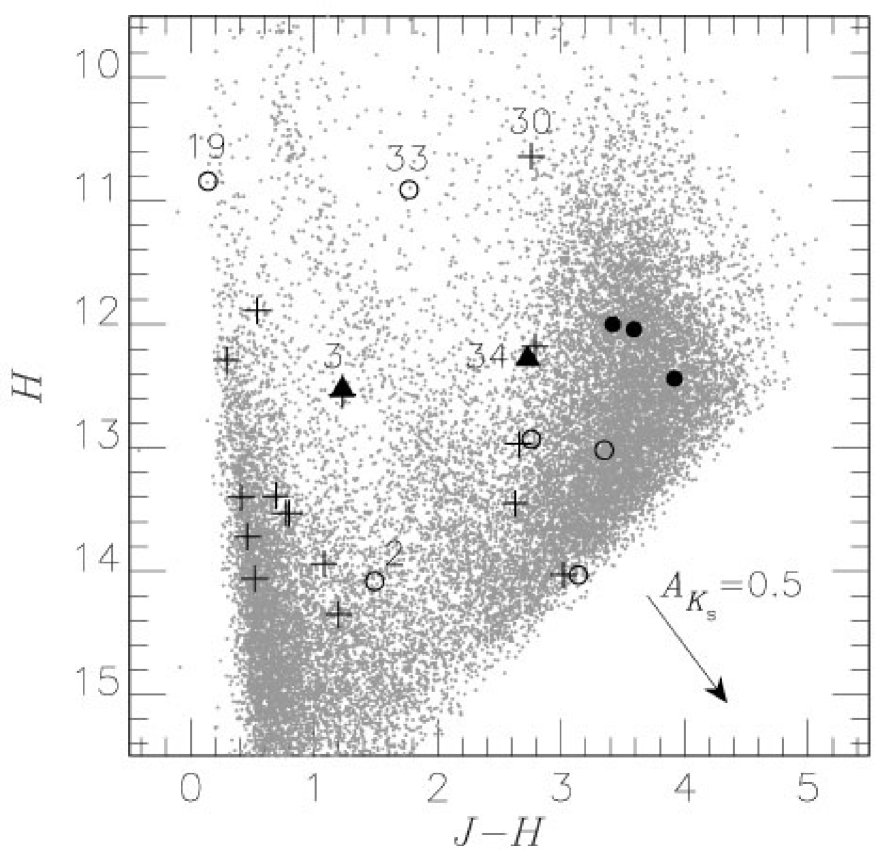
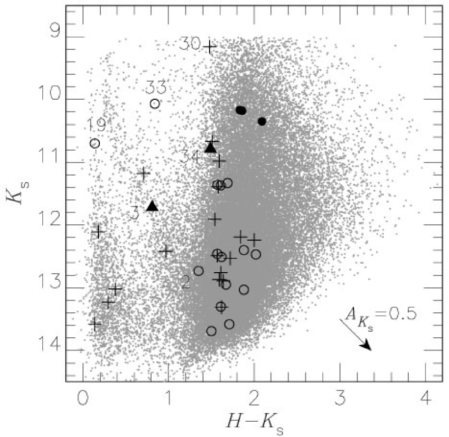
Figure 4: Colour-magnitude diagrams: $J-H$ vs $H$ (left) and $H-K_{\mathrm{s}}$ vs $K_{\mathrm{s}}$ (right). The short-period variables are indicated by symbols depending on the classified variable types: eclipsing variables by plus symbols, CCEPs by filled circles, T2Cs by open circles and the other variables by triangles, while grey dots plot other objects. The numbered objects are discussed in the text. The arrow indicates the reddening vector corresponding to $A_{K_{\mathrm{s}}}=0.5$ mag.

Eclipsing binaries, plus symbols in Fig. 4, are separated roughly into two groups, around the foreground main sequence or on the giant branch of the bulge. A few points exist in the intermediate colour range, #8, #36 and #41, but their colours are affected by the crowding (see their $M$flag in Table 2). The colours of the redder group suggest that they have large interstellar extinction and are thus distant and likely in the GC region. Excluding those affected by the crowding, this group includes #17, #21, #25, #27, #30, #37, #38, #42 and #43. They tend to have longer orbital periods than the bluer binaries. The brightest of the reddened binaries, #30 ($P=26.8$ d), is of particular interest. It was reported as an O-type supergiant located near the GC (Mauerhan et al., 2010), but we find that it is a binary system. Furthermore, its asymmetric light curve suggests that the system has an eccentric orbit. Since the other reddened binaries may well be at the distance of the GC, they are also interesting objects for further study.

The triangle for #3 falls near the diagonal sequence of the red clump giants in the disk (Lucas et al., 2008), where the RR Lyr and $\delta$ Sct stars in the foreground are roughly expected. On the other hand, #34 is highly reddened and relatively bright, although the images in the $H$ and $K_{\mathrm{s}}$ bands indicate that the photometry may be affected by crowding. Its distance would be 3.6 kpc if it were an overtone CCEP, and the distance would be smaller otherwise. Therefore it is much closer than the GC, and yet the extinction is quite high, $A_{K_{\mathrm{s}}}\sim 2$ mag. These values may be subject to the uncertainty due to the crowding, but it would not change the conclusion that this object is in the foreground of the GC. The nature of the star remains to be investigated.

4 Discussion

4.1 Samples of Type II Cepheids

Our catalogue includes 16 T2Cs; 14 are located in the bulge and two in the foreground (#19 and #33). In the following discussion, we consider 14 objects as our sample of T2Cs in the bulge unless otherwise mentioned. We found few T2Cs with short period ($P<5$ d). In fact our survey was not deep enough to detect such objects. The PLR enables us to tell if the detection limit is deep enough to detect a Cepheid with a given period, foreground extinction and distance. Fig. 5 illustrates the range in the parameter plane of $(\log P,A_{K_{\mathrm{s}}})$ where we should be able to detect T2Cs at the distance of the GC. For example, a T2C with $\log P=1$ could not be detected if the foreground extinction is larger than $A_{K_{\mathrm{s}}}=2$ mag. Considering that the majority of the objects near the GC are reddened more strongly, our survey is far from complete. In Fig. 5, several of the detected T2Cs seem to be beyond the detection limit in the $H$ band or even in the $K_{\mathrm{s}}$ band. This happens because the limiting magnitude depends on the crowdedness which varies within our survey region. Our survey region includes the extremely crowded region near Sgr A^∗ and also sparse regions towards dark cloud lanes.

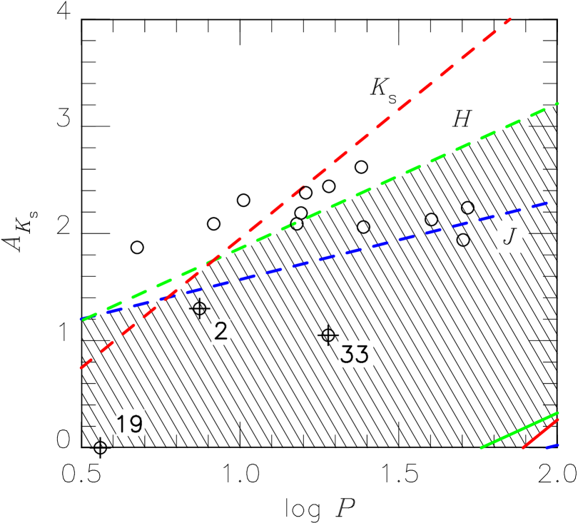
Figure 5: A schematic diagram to show the range, in the parameter space of $(\log P,A_{K_{\mathrm{s}}})$, where we can detect T2Cs located at the GC distance. Dashed lines show the detection limits for $JHK_{\rm s}$, while solid lines indicate the saturation limits though scarcely relevant. Blue green and red lines correspond to the limits in $J$, $H$ and $K_{\mathrm{s}}$, respectively. The shaded region illustrates the range for which the T2Cs are detected in two or more filters. The open circles are plotted for the $(\log P,A_{K_{\mathrm{s}}})$ values of the T2Cs we discovered in this work. Star #2 (uncertain photometry) and the stars #19 and #33 (foreground) are indicated.

Recently, Soszyński et al. (2011) found a rich population of T2Cs in the outer bulge towards low-extinction regions away from the Galactic plane. We combined their catalogue with the 2MASS near-infrared catalogue (Skrutskie et al., 2006) with the tolerance radius of 1 arcsec. There are 156 BL Her, 128 W Vir and 51 RV Tau objects in the OGLE-III catalogue, and we found 97, 117 and 49 counterparts for the three types of T2Cs respectively (263 in total, Table 7). Because of their faintness, a significant fraction of the BL Her stars were not detected in 2MASS. In addition, the 2MASS catalogue indicates that photometric accuracies for quite a few objects are limited because of confusion or other reasons. Considering the quality flag, the blend flag and the confusion flag (Qflag, Bflag and Cflag in Table 7), there remain 166, 138 and 138 measurements in the $JHK_{\rm s}$ bands with good photometric quality. We discriminate these ”good” magnitudes from the others below. In addition, we use the $I$-band light curves obtained by the OGLE-III survey to make phase corrections to convert the single-epoch 2MASS magnitudes into mean magnitudes. The same method was described and used in Matsunaga et al. (2009a, 2011a). Table 7 lists the size of the correction, $\Delta_{\phi}$, which is to be added to the 2MASS magnitudes for each object. Some $I$-band light curves show a large scatter, and we do not apply the phase correction for those T2Cs (mainly RV Tau stars, with $\Delta_{\phi}=99.999$ in Table 7).

Table 7: 2MASS counterparts for the OGLE-III type II Cepheids in the bulge. The table lists the period $P$ and the 2MASS $JHK_{\rm s}$ magnitudes as well as the quality flags: Qflag=the photometric quality flag, Bflag=the blend flag, and Cflag=the confusion flag (Skrutskie et al., 2006). In the last column listed are the phase correction $\Delta_{\phi}$ we obtained with the OGLE $I$-band light curves (see the text). This is the first 10 lines of the full catalogue which will be available in the online version of the article (see Supporting Information).

OGLE ID	$P$	2MASS ID	$J$	$H$	$K_{\mathrm{s}}$	Qflag	Bflag	Cflag	$\Delta_{\phi}$
	(days)		(mag)	(mag)	(mag)				(mag)
OGLE-BLG-T2CEP-001	3.9983508	17052035-3228176	12.904	12.412	12.273	AAA	111	000	$0.160$
OGLE-BLG-T2CEP-002	2.2684194	17061499-3301275	13.130	12.713	12.587	AAA	111	000	$-0.050$
OGLE-BLG-T2CEP-003	1.4844493	17084014-3254104	13.826	13.457	13.276	AAA	111	00c	$0.295$
OGLE-BLG-T2CEP-004	1.2118999	17131083-2905453	13.817	13.355	13.248	AAA	111	000	$0.052$
OGLE-BLG-T2CEP-006	7.6379292	17142541-2846465	12.213	11.863	11.682	AAA	111	000	$0.266$
OGLE-BLG-T2CEP-007	1.8173297	17235478-2902378	14.293	13.607	13.426	AAA	111	000	$-0.200$
OGLE-BLG-T2CEP-008	1.1829551	17242093-2755493	14.573	99.999	99.999	AUU	200	c00	$0.091$
OGLE-BLG-T2CEP-009	1.8960106	17242227-2927352	14.218	13.539	13.245	AAA	112	0dc	$-0.159$
OGLE-BLG-T2CEP-010	1.9146495	17270554-2536015	13.671	13.143	12.989	AAA	111	000	$0.138$
OGLE-BLG-T2CEP-011	15.3886022	17271765-2538234	12.006	11.208	10.995	AAA	111	000	$-0.300$

4.2 Period distribution and surface density

The period distributions of our T2Cs and the OGLE-III sample are shown in Fig. 6. Most of our sample have long periods ($P>10$ d). This bias is caused by the detection limit of our survey as mentioned above. In contrast, with more than 300 T2Cs, the OGLE-III sample clearly shows the distinct groups of BL Her, W Vir, RV Tau stars. Such a feature is well seen in the T2C samples of the Magellanic Clouds but not in that of globular clusters (see fig. 5 in Matsunaga et al. 2011a).

In addition, there are significantly more W Vir stars than RV Tau stars and the periods of W Vir stars show a broad, or even two distinct, peak(s), both of which are similar to the case of the LMC T2Cs. The number of BL Her stars is even larger than W Vir stars, i.e. $N_{\rm WV}/N_{\rm BL}=0.82\pm 0.14$ (error from Poisson noise). This ratio falls between the case of the LMC (1.25) and the SMC (0.6) given in Matsunaga et al. (2011a). The reason for these variations in the T2C populations is presumably related to age and/or metallicity, but the lack of theoretical models for T2Cs prevents us from further discussion.

Figure 6: Histograms of periods for the T2Cs in the bulge: the top panel for our sample and the bottom for the OGLE-III sample (Soszyński et al., 2011). Vertical lines show the thresholds, 5 and 20 d, used to divide BL Her, W Vir and RV Tau variables.

It is of interest to examine the surface density of T2Cs in the bulge. We detected 11 T2Cs with $P>15$ d, which leads to the density of 66 deg^-2 considering the area of our survey towards the GC (1/6 deg^-2). However, our survey was not complete even for the relatively long-period T2Cs because of thick dark nebulae (Fig. 5), and the above density is an underestimate thus indicated by the arrow in Fig. 7. For the outer bulge region, we obtained the surface density of T2Cs for each OGLE-III region. Fig. 7 plots the surface densities of the OGLE-III T2Cs with $P>15$ d (filled circles) and all T2Cs (crosses) in each field against the angular distance from the GC. We consider only the fields in the range of $|l|<2^{\circ}$ and $|b|<4^{\circ}$ where the density is high enough. The profile in Fig. 7 shows, in effect, the variation along the minor axis. In addition, Fig. 8 shows a similar plot of the density profile for Miras. Matsunaga et al. (2011b) found 547 Miras with period determined in the same IRSF survey field, among which 251 objects have periods less than 350 d. Whilst the Miras have a broad range of age (from $\sim 10$ Gyr to 1 Gyr or even younger), such short-period Miras are found in globular clusters (Frogel & Whitelock, 1998) and considered to belong to the old stellar population. The number of the short-period Miras towards the GC field corresponds to a surface density of 2200 deg^-2. The surface densities for the outer region were obtained using the catalogue of the OGLE-II Miras compiled by Matsunaga, Fukushi & Nakada (2005). In Fig. 8, the density profile for the OGLE-II Miras is well represented by the exponential law, $N\sim\exp(-0.24r)$. This exponential fits the OGLE-II points better than a de Voucouleurs law or a Sersic law, $\log N\sim R^{1/n}$, with $n=2$. Note that the exponential and the de Voucouleurs law correspond to the Sersic law with $n=1$ and $n=4$ respectively. In contrast, the lower limit inferred by our sample is higher than the exponential law predicted by the OGLE-II Miras. This excess agrees with the idea that an additional population of Miras exist in the nuclear bulge, the disk-like system within $\sim 200$ pc. Although the density profile for T2Cs is uncertain due to the small number, our result on the T2C distribution also suggests that the nuclear bulge holds an additional group of T2Cs in the central region.

Figure 7: Density profile of T2Cs in the bulge. Crosses and filled circles indicate the surface densities [deg^-2] of all T2Cs and those with $P>15$ d (Soszyński et al., 2011) in the OGLE-III fields with $|l|<2^{\circ}$ and $|b|<4^{\circ}$. The lower limit of the density of T2Cs with $P>15$ d towards the GC is indicated by the arrow. The exponential law indicated by the straight lines gives reasonable fits to the OGLE-III points.

Figure 8: Same as Fig. 7, but for Miras. Crosses and filled circles indicate the surface densities [deg^-2] of all Miras with known periods and those with $P<350$ d (Matsunaga et al., 2009b) in the OGLE-II fields with $|l|<2^{\circ}$ and $|b|<4^{\circ}$. The lower limit of the density of Miras with $P<350$ d towards the GC is indicated by the arrow. The exponential law indicated by the straight lines gives reasonable fits to the OGLE-II points.

4.3 The distance to the GC

There have been a considerable number of estimates of the distance to the Galactic Centre based on stellar distance indicators. Many of these rely on data from the general region of the Galactic bulge and may, to a greater or lesser degree, be affected by the bar-like and other structure of the bulge. In this section, we concentrate on data obtained in the areas close to the Centre which should be free of any such effects.

In view of the importance of reddening in this region we use a reddening free PLR in $H$ and $K_{\mathrm{s}}$,

$$W(HK_{\mathrm{s}})=K_{\mathrm{s}}-1.44(H-K_{\mathrm{s}}),$$ (12)

where the coefficient is taken from the extinction law found by Nishiyama et al. (2006a). As a preliminary we compare our T2C results with those from the OGLE-III survey in the general bulge. Fig. 9 plots $W(HK_{\mathrm{s}})$ against the period for both our sample and the OGLE-III sample with $H$ and $K_{\mathrm{s}}$ magnitudes. Of our sample, 13 are indicated by the filled circles, whereas the crosses indicate two foreground stars (#19 and #33) and #2 with uncertain photometry. The grey symbols show the OGLE-III objects (filled circles for those with good $H/K_{\mathrm{s}}$ magnitudes and open circles for others). The linear relations drawn in the Fig. 9 are obtained with the T2Cs in globular clusters (filled line; Matsunaga et al. 2006) and those in the LMC (dashed line; Matsunaga et al. 2009a) but with a shift considering the approximate distance moduli of the LMC (18.50 mag) and the bulge (14.50 mag). Most of our T2Cs except the crosses (#2, #19 and #33) lie close together with the samples of the OGLE-III catalogue in the vicinity of the GC, $\sim 8$ kpc (Fig. 3). In contrast, #26 ($\log P=1.21$) seems brighter than the relation for other stars. If it is a normal T2C it lies in the foreground of the bulge while it may be a peculiar W Vir stars brighter than regular W Vir stars. Several objects in the OGLE-III are also brighter than the others, and their nature needs to be investigated.

We now concentrate on our T2Cs, which are in the vicinity of the GC, and whose periods fall within the range of W Vir stars. Previous work found that the PLRs of BL Her/RV Tau stars may be different between different galaxies (Matsunaga et al. 2009a, 2011a; Soszyński et al. 2011), although we did not confirm significant deviation of our T2C samples from the PLR of those in globular clusters (Fig. 9). We obtained the average modulus of $\mu_{0}=14.38\pm 0.13$ mag, based on 5 W Vir stars ($5\geq P\geq 20$ d) excluding #26, under the assumption of $\mu_{0}{({\mathrm{LMC}})}=18.50$ mag. The errors in the above estimates account just for statistical errors, and we need to consider systematic uncertainties. Our estimates are affected by errors in the extinction law and the LMC distance as well as the possible population effect on the PLR. We adopt an uncertainty of 0.05 mag for the LMC modulus and 0.07 mag for the adopted reddening law as we did in Paper I for the GC Miras. The results of Matsunaga et al. (2006) and Matsunaga et al. (2011a) suggest that any population effect on the PLR of T2Cs (W Vir stars) is small. Nevertheless, to be conservative we adopt an uncertainty of 0.07 mag for this. Considering these errors and the above estimates, the current sample of T2Cs results in an estimate of the GC distance modulus to be $14.38\pm 0.17$ mag. There is a further uncertainty due, as discussed above, to our detection limit. This might result in the modulus being slightly underestimated. With the same survey data, we obtained the distances to Miras (Paper I) and CCEPs (Paper II). Adopting $\mu_{0}{({\mathrm{LMC}})}=18.50$ mag, the average of the distances to Miras gives $\mu_{0}{({\mathrm{GC}})}=14.63\pm 0.11$ mag. On the other hand, the calibration of CCEPs are based on the nearby calibrators and the average of the three distances leads to $\mu_{0}{({\mathrm{GC}})}=14.49\pm 0.12$ mag. The error budgets for these estimates are discussed in Papers I and II.

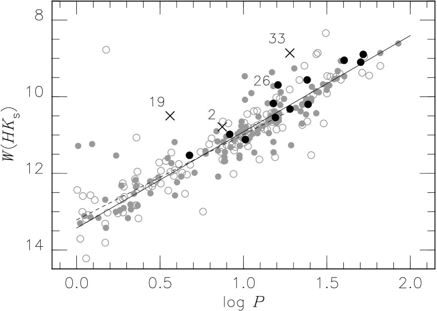
Figure 9: The $\log P$-$W(HK_{\mathrm{s}})$ relation for T2Cs in the bulge. Black filled circles indicate our T2Cs, but crosses indicate two foreground stars (#19 and #33) and #2 with uncertain photometric result. The stars in the OGLE III catalogue (Soszyński et al., 2011) are also plotted as the grey symbols, of which the open circles are used for the objects with uncertain 2MASS photometry or no phase correction applied (see text) and filled circles for the others. Dashed and filled relations plot the $\log P$-$W(HK_{\mathrm{s}})$ relations for the LMC T2Cs (Matsunaga et al., 2009a) and those in globular clusters (Matsunaga et al., 2006), respectively, but after the distance effect corrected assuming $\mu_{0}$(LMC)=18.50 mag and $\mu_{0}$(bulge)=14.50 mag.

$JHK_{\rm s}$ observations of red clump stars in the region around the Galactic Centre were obtained by Nishiyama et al. (2006b) using the IRSF/SIRIUS. Recently, Laney, Joner & Pietrzyński (2012) obtained new high-precision $JHK_{\rm s}$ magnitudes of red clump giants with the Hipparcos parallaxes, which gives a new calibration of the red clump. Nishiyama et al. (2006b) adopted $(H-K_{\mathrm{s}})_{0}=0.07$ and $K_{\mathrm{s}}=-1.59$ from theoretical isochrones by (Bonatto, Bica & Girardi, 2004), whereas Laney et al. (2012) obtained $(H-K_{\mathrm{s}})_{0}=0.123$ and $K_{\mathrm{s}}=-1.613$. Using this new calibration leads to $\mu_{0}{({\mathrm{GC}})}=14.53\pm 0.10$ mag, that is $8.05\pm 0.37$ kpc, without any population effect taken into account. There is a large scatter in metallicities of red clump giants in the bulge and the median metallicity seems slightly higher than the solar abundance (Hill et al., 2011). The error, adopted from Nishiyama et al. (2006b), includes and is affected by the uncertainty of a possible population effect.

These estimates based on near-IR data of stellar distance indicators in areas close to the Centre are compared with the results from kinematic methods in Fig. 10. These latter methods are: the Kepler rotation of the star S2 around Sgr A^∗ (Gillessen et al., 2009), the statistical parallax method applied to the central stellar cluster (Trippe et al., 2008) and the parallax of Sgr B (Reid et al., 2009). The photometric and kinematic determinations are in satisfactory agreement and indicate a value of $R_{0}$, close to 8.0 kpc. The uncertainty in the reddening law is the dominant remaining error for the photometric distances discussed here. Thus the agreement of the photometric and kinematic results lends support to the reddening law of Nishiyama et al. (2006a). For a typical value of $E_{H-K_{\mathrm{s}}}=1.8$, for instance, the Nishiyama value of $A_{K_{\mathrm{s}}}$ is 2.5 mag whereas the Rieke & Lebofsky (1985) law gives 3.2 mag and would lead to an unacceptably small value of $R_{0}$(GC).

Figure 10: Estimates of the distance $R_{0}$ to the GC based on various methods (see the text for references). Error bars include the statistical and systematic uncertainties.

5 Summary

Through our near-IR survey of stellar variability towards the GC, 45 short-period variables have been discovered. Their light curves are investigated to determine the variable types, and for the Cepheid candidates their distances and foreground extinctions are also considered based on the PLRs. Most of the objects are reasonably classified: three CCEPs, 16 T2Cs, 24 eclipsing binaries, and two others. The numbers of T2Cs and short-period Miras in our survey region are higher than the surface density following the exponential law which fits the distribution of T2Cs and Miras in the outer bulge. This strongly suggests that the nuclear bulge hosts a significant population of old stars ($\geq 10$ Gyr). We also discuss the distance to the Galactic Centre based on stellar distance indicators in the central region. These are insensitive to problems associated with the three dimensional structure of the bulge which may affect other determinations. Our main result is close to 8 kpc and agrees well with kinematic estimates. Since the photometric results are rather sensitive to the infrared reddening law, the result give support to the reddening law of Nishiyama et al. (2006a) which we adopted.

Supporting information

Additional Supporting Information may be found in the online version of this article.
Table 3. The released table of light variation for the catalogued variables.
Table 7. 2MASS counterparts for the OGLE-III type II Cepheids in the bulge.

References

- Benedict et al. (2007) Benedict G. F. et al. 2007, AJ, 133, 1810
- Benedict et al. (2011) Benedict G. F. et al. 2011, AJ, 142, 187
- Bonatto et al. (2004) Bonatto Ch., Bica E., Girardi L., 2004, A&A, 415, 571
- Caldwell & Coulson (1985) Caldwell J. A. R., Coulson I. M., 1985, MNRAS, 212, 879
- Clarkson et al. (2011) Clarkson W. I. et al. 2011, ApJ, 735, 37
- Feast (2012) Feast M. W., 2012, in Gilmore G., ed, Planets, Stars and Stellar Systems, Vol. 5, Stellar Systems and Galactic Structure. Springer, Berlin, in press
- Figer et al. (2004) Figer D. F., Rich R. M., Kim S. S., Morris M., Serabyn E., 2004, ApJ, 601, 319
- Frogel & Whitelock (1998) Frogel J. A., Whitelock P. A., 1998, AJ, 116, 754
- Genzel et al. (2003) Genzel R. et al. 2003, ApJ, 594, 812
- Genzel et al. (2010) Genzel R., Eisenhauer F., Gillessen S., 2010, Rev. Modern Phys., 82, 3121
- Ghez et al. (2008) Ghez A. M. et al. 2008, ApJ, 689, 1044
- Gillessen et al. (2009) Gillessen S., Eisenhauer F., Fritz T. K., Bartko H., Dodds-Eden K., Pfuhl O., Ott T., Genzel R., 2009, ApJ, 707, L114
- Hill et al. (2011) Hill V. et al. 2011, A&A, 534, A80
- Laney et al. (2012) Laney C. D., Joner M. D., Pietrzyński G., 2012, MNRAS, 419, 1634
- Laney & Stobie (1993) Laney C. D., Stobie R. S., 1993, MNRAS, 260, 408
- Launhardt et al. (2002) Launhardt R., Zylka R., Mezger P. G., 2002, A&A, 384, 112
- Lucas et al. (2008) Lucas P. W. et al. 2008, MNRAS, 391, 136
- Matsunaga et al. (2005) Matsunaga N., Fukushi H, Nakada Y., 2005, MNRAS, 364, 117
- Matsunaga et al. (2006) Matsunaga N. et al. 2006, MNRAS, 370, 1979
- Matsunaga et al. (2009a) Matsunaga N., Feast M. W., Menzies J. W., 2009a, MNRAS, 397, 933
- Matsunaga et al. (2009b) Matsunaga N., Kawadu T., Nishiyama S., Nagayama T., Hatano H., Tamura M., Glass I. S., Nagata T., 2009b, MNRAS, 399, 1709 (Paper I)
- Matsunaga et al. (2011a) Matsunaga N., Feast M. W., Soszyński I., 2011a, MNRAS, 413, 223
- Matsunaga et al. (2011b) Matsunaga N. et al. 2011b, Natur, 477, 188 (Paper II)
- Mauerhan et al. (2010) Mauerhan J. C., Cotera A., Dong H., Morris M. R., Wang Q. D., Stolovy S. R., Lang C., 2010, ApJ, 725, 188
- Morris & Serabyn (1996) Morris M., Serabyn E., 1996, ARA&A, 34, 645
- Nagashima et al. (1999) Nagashima C. et al. 1999, in Nakamoto T., ed, Proc. Star Formation 1999. Nobeyama Radio Observatory, Nagano, p. 397
- Nagayama et al. (2003) Nagayama T. et al. 2003, in Iye M., Moorwood A. F. M., eds, SPIE Vol. 4841, Instrument Design and Performance for Optical/Infrared Ground-Based Telescopes. SPIE, Bellingham, p. 459
- Nakada et al. (1991) Nakada Y., Deguchi S., Hashimoto O., Izumiura H., Onaka T., Sekiguchi K., Yamamura I., 1991, Natur, 353, 140
- Nishiyama et al. (2006a) Nishiyama S. et al. 2006a, ApJ, 638, 839
- Nishiyama et al. (2006b) Nishiyama S. et al. 2006b, ApJ, 647, 1093
- Ott et al. (1999) Ott T., Eckart A., Genzel R., 1999, ApJ, 523, 248
- Peeples et al. (2007) Peeples M. S., Stanek K. Z., DePoy D. L., 2007, Acta Astron., 57, 173
- Poleski et al. (2010) Poleski R. et al. 2010, Acta Astron., 60, 1
- Rafelski et al. (2007) Rafelski M., Ghez A. M., Hornstein S. D., Lu J. R., Morris M., 2007, ApJ, 659, 1241
- Reid et al. (2009) Reid M. J., Menten K. M., Zheng X. W., Brunthaler A., Xu Y., 2009, ApJ, 705, 1548
- Rieke & Lebofsky (1985) Rieke G. H., Lebofsky M. J., 1985, ApJ, 288, 618
- Sandage & Tammann (2006) Sandage A., Tammann G. A., 2006, ARA&A, 44, 93
- Serabyn & Morris (1996) Serabyn E., Morris M., 1996, Natur, 382, 602
- Skrutskie et al. (2006) Skrutskie M. F. et al. 2006, AJ, 131, 1163
- Soszyński et al. (2008a) Soszyński I. et al. 2008a, Acta Astron., 58, 163
- Soszyński et al. (2008b) Soszyński I. et al. 2008b, Acta Astron., 58, 293
- Soszyński et al. (2009) Soszyński I. et al. 2009, Acta Astron., 59, 1
- Soszyński et al. (2011) Soszyński I. et al. 2011, Acta Astron., 61, 285
- Stanek et al. (1994) Stanek K. Z., Mateo M., Udalski A., Szymański M., Kałużny J., Kubiak M., 1994, ApJ, 429, L73
- Tamura et al. (1996) Tamura M., Werner M. W., Becklin E. E., Phinney E. S., 1996, ApJ, 467, 645
- Trippe et al. (2008) Trippe S. et al. 2008, A&A, 492, 419
- van Leeuwen et al. (2007) van Leeuwen F., Feast M. W., Whitelock P. A., Laney C. D., 2007, MNRAS, 379, 723
- Whitelock & Catchpole (1992) Whitelock P. A., Catchpole R., 1992, in Blitz L., ed, The center, bulge, and disk of the Milky Way. Kluwer, Dordrecht, p. 103
- Yusef-Zadeh et al. (2009) Yusef-Zadeh F. et al. 2009, ApJ, 702, 178
- Zoccali et al. (2003) Zoccali M. et al. 2003, A&A, 399, 931