The full-tails gamma distribution applied to model extreme values

Abstract.

In this article we show the relationship between the Pareto distribution and the gamma distribution. This shows that the second one, appropriately extended, explains some anomalies that arise in the practical use of extreme value theory. The results are useful to certain phenomena that are fitted by the Pareto distribution but, at the same time, they present a deviation from this law for very large values. Two examples of data analysis with the new model are provided. The first one is on the influence of climate variability on the occurrence of tropical cyclones. The second one on the analysis of aggregate loss distributions associated to operational risk management.

Keywords: Exponential models. Heavy tailed distributions. Pareto distribution. Power-law distribution. Type III distribution. Operational risk models.

1. Introduction

The extreme value theory is used by many authors to model exceedances in several fields such as hydrology, insurance, finance and environmental science, see Furlan (2010), Coles and Sparks (2006), Moscadelli (2004). However, the theory shows some surprises in practical applications. For instance, Dutta and Perry (2006) observed, in an empirical analysis of models for estimating operational risk, that even when Pareto distribution fit the data it may result in unrealistic capital estimates (sometimes more than 100% of the asset size), see also Degen, et al. (2007). In other instances despite being well-founded the power law-distribution, as in Corral, et al. (2010), it may happen that it works in the central region but not for larger values. These challenges should motivate us to find new models that describe the characteristics of the data rather than limit the data so that it matches the characteristics of the model (Dutta and Perry, 2006).

The peaks over threshold (PoT) method for estimating high quantiles is based on the Pickands-Balkema-DeHaan Theorem, see McNeil, et al. (2005) and Embrechts, et al. (1997). Hence, in practice, the conditional distribution of any random variable over a high threshold is approximated by a generalized Pareto distribution (GPD). This result is a mathematical solution to the question, but the practical problem whether the threshold is high enough still remains.

In this paper a new statistical approach for estimating high quantiles is provided for non-light tails data sets. It is shown that the Pareto distribution is nested in the statistical model here called full-tails gamma (FTG) distribution. FTG model is a scale parameter family of distributions on $\left(0,\infty\right)$ closed by truncation, Hence, it allows us to find distributions so close to the Pareto distribution as determined by the data, but with greater flexibility, extending the distributions for non-light tails provided by GPD. With the current specialized computer programs for statistical analysis is not difficult to deal with the FTG distribution, since the incomplete gamma function and its derivatives are now easily available, see Abramowitz and Stegun (1972). The work of pioneers like Chapman (1956) must be viewed in this way. Another approach for lighter tails is in Akinsete, et al. (2008).

The FTG distribution is related to very old families of distributions as the Pareto III distribution, see Arnold (1983, pp 3) and Davis et al (1979). The gamma distribution is one of the most studied families of distributions, since Fisher (1922). For life theory and reliability the two-parameter right truncated gamma distribution is usually considered since Chapman (1956). Den Broeder (1955) considered the left truncated gamma distribution but with known scale parameter. Stacy (1962) introduced a three-parameter generalized gamma distribution which includes, as special cases, the two-parameter gamma and the two-parameter Weibull. Harter (1967) extends the model to a four-parameter family, by including a location parameter. Hedge and Dahiya (1989) obtain necessary and sufficient conditions for the existence of the MLE of the parameters of a right truncated gamma distribution. The right truncated gamma with unknown origin is studied by Dixit and Phal (2005). For simulation of right and left truncated gamma distributions, see Philippe (1997). Also in physics literature the FTG distribution appears related to the power-law with (exponential) cut off, see Clauset et al (2009) or Sornette (2006), however, the models are not the same.

In Section 2, FGT distribution is introduced, showing that the domain of parameters includes the gamma distribution and the Pareto distribution (Theorem 1) in the boundary. Proposition 2 provides a clear interpretation of its three parameters $\left(\alpha,\theta,\rho\right)$. The FTG distribution for $\alpha>0$ is the left truncated gamma distribution relocated to the origin . The FTG distribution for $\alpha\leq 0$ appears as the full exponential model generated from a canonical statistic. Section 3 describes the most basic statistical properties of the FTG, as the moments generating function, a simulation method and the standard tools for MLE.

In Section 4, we provide applications of the FTG exemplify that are usually fitted by Pareto distribution. The first one on the influence of climate variability and global warming on the occurrence of tropical cyclones, see Corral, et al. (2010). Here, classical goodness of fit test rejects Pareto distribution but it offers no alternative to that model. The alternative is here provided by the FTG distribution.

The second example deals with the analysis of aggregate loss distributions associated to operational risk management, see Degen, et al. (2007). The concept of operational risk is founded in the Basel II accord of 1999, that has been widely adopted around the world as a regulatory requirement by central banks. The focus on systemic risk, precipitated by the current crisis, has elevated operational risk management to greater prominence. Risk capital, under the PoT approach, has been calculated here with Pareto and FTG distributions. Table 3 shows that Pareto distribution provides unrealistic and highly unstable estimations, however, FTG distribution provides more realistic and much more stable risk capital estimations.

2. The full-tails gamma distribution

The FTG distribution is the three-parameter family of continuous probability distributions, with support on $(0,\infty)$, defined by $\alpha\in\mathbb{R},\theta>0,\rho>0$ by

(2.1) $$f\left(x;\alpha,\theta,\rho\right)=\theta\left(\rho+\theta x\right)^{\alpha-1}\exp(-(\rho+\theta x))/\Gamma(\alpha,\rho).$$

where $\Gamma\left(\alpha,\rho\right)$ is the (upper) incomplete gamma function, see Abramowitz and Stegun (1972),

(2.2) $$\Gamma\left(\alpha,\rho\right)=\int_{\rho}^{\infty}t^{\alpha-1}e^{-t}dt,$$

in particular $\Gamma\left(\alpha,0\right)=\Gamma\left(\alpha\right)$ is the gamma function. The FTG distribution extends to some boundary parameters as shall seen bellow.

If $\alpha>0,\theta>0$ and $\rho=0$, the family $\left(\ref{FTG}\right)$ clearly extends to the probability density function of the gamma distribution, defined by

(2.3) $$g\left(x;\alpha,\theta\right)=\theta^{\alpha}x^{\alpha-1}\exp\left(-\theta x\right)/\Gamma\left(\alpha\right)$$

For $\alpha>0$ the FTG  is the left truncated gamma distribution relocated to the origin, or equivalently it is a tail of gamma distribution. Note that in this paper, tail is used in sense of conditional exceedances over a threshold. More exactly, suppose $F(x)$ is a absolutely continuous cumulative distribution function of a non negative random variable, $X$. The probability density function of the exceedances of $X$ at $u>0$ is defined by

(2.4) $$f_{u}\left(x\right)=f\left(x+u\right)/(1-F(u))$$

where $f\left(x\right)=F^{\prime}\left(x\right)$. If $\alpha>0$ and $\rho>0$, then $\left(\ref{FTG}\right)$ is the probability density function of the exceedances of a gamma distribution at $\sigma>0$, with $\sigma=\rho/\theta$

(2.5) $$g_{\sigma}\left(x;\alpha,\theta\right)=\theta^{\alpha}\left(x+\sigma\right)^{\alpha-1}\exp\left(-\theta\left(x+\sigma\right)\right)/\Gamma\left(\alpha,\sigma\theta\right).$$

The probability density function of the Pareto distribution, defined for $x>0$, is

(2.6) $$p\left(x;\alpha,\sigma\right)=-\alpha\sigma^{-1}\left(1+x/\sigma\right)^{\alpha-1},$$

where $\alpha<0$ and $\sigma>0$. This parameterization will be used to show that the Pareto distribution appears in this boundary of the FTG distribution.

Theorem 1.

Let $\sigma=\rho/\theta>0$ fixed in $\left(\ref{FTG}\right)$ and $\alpha<0$. If $\rho$ tends to zero, then the probability density function $\left(\ref{FTG}\right)$ tends to the probability density function of the Pareto distribution (2.6) in $L^{1}$ norm. Moreover, the convergence extends to the moments, provided the corresponding moments for Pareto distribution are finite.

Proof.

Observe that if $\rho$ tends to $0$, then $\theta$ tends to $0$, since $\sigma=\rho/\theta>0$ is fixed. Using $\theta=\rho/\sigma$,

$$f(x;\alpha,\theta,\rho)=\rho^{\alpha}\sigma^{-1}(1+x/\sigma)^{\alpha-1}\exp(-\rho(1+x/\sigma))/\Gamma(\alpha,\rho)$$

converges pointwise to the probability density function $\left(\ref{par}\right)$, since the property (5.1.23) of Abramowitz and Stegun (1972), under the assumptions,

(2.7) $$\lim_{\rho\to 0}\rho^{\alpha}/\Gamma(\alpha,\rho)=-\alpha$$

holds. Observe that for $\rho$ small

$$f(x;\alpha,\theta,\rho) = \rho\sigma^{-1}(1+x/\sigma)^{\alpha-1}\exp(-\rho(1+x/\sigma))/\Gamma(\alpha,\rho)$$

$$\leq -2\alpha\sigma^{-1}(1+x/\sigma)^{\alpha-1}=2p\left(x;\alpha,\sigma\right)$$

since from the limit $\left(\ref{lim}\right)$ we can consider the boundedness $\rho^{\alpha}/\Gamma(\alpha,\rho)\leq-2\alpha$. Finally, from the dominated convergence theorem we obtain the convergence in $L^{1}$. Moreover, whenever the moments of Pareto distribution are finite, the convergence extends to these moments. ∎

Therefore, the family $\left(\ref{FTG}\right)$ has the boundary parameter sets corresponding to the gamma distribution:$\left\{\alpha>0,\theta>0,\rho=0\right\}$ and the Pareto distribution:$\left\{\alpha<0,\theta=0,\sigma>0\right\}$. Summarizing, the FTG distribution$\left(\ref{FTG}\right)$ includes the gamma distribution, the truncated gamma distribution $\left(\alpha>0\right)$, its extension to $\alpha{\color[rgb]{0,0,1}\leq}0$ and the Pareto distribution, see Figure 2.1.

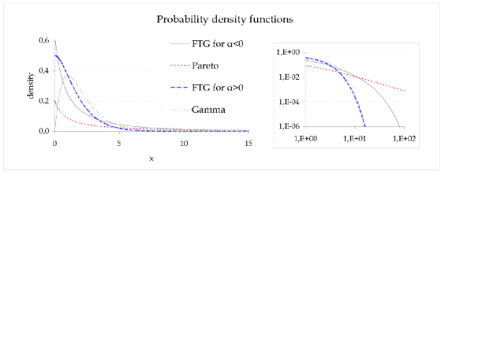
Figure 2.1. The left shows some probability density functions in FTG family. The FTG with $\alpha=2$, $\sigma=1$ and $\theta=1$ corresponds to the tails of a gamma and the FTG for $\alpha=-0.2$, $\sigma=1$ and $\theta=0.1$ is not. For the boundary parameter sets of the family, we consider gamma with $\alpha=2$ and $\theta=1$ and Pareto with $\alpha=-0.2$ and $\sigma=1$. The right shows the same plot in common logarithm for the tail of the functions. We see exponential decay except for Pareto probability density function.

Proposition 2.

Let $X$ be a random variable distributed as $FTG(\alpha,\theta,\rho)$, then

(a) For $\lambda>0$, the random variable $\lambda X$ is distributed as $FTG\left(\alpha,\theta/\lambda,\rho\right)$.

(b) For any threshold, $u>0$, the threshold exceedances, $X_{u}$ is distributed as $FTG(\alpha,\theta,\rho+\theta u).$

Proof.

The first result holds from the probability density function of $\lambda X$ for $\lambda>0$,

$$f\left(x/\lambda;\alpha,\theta,\rho\right)/\lambda=(\theta/\lambda)\left(\rho+\theta x/\lambda\right)^{\alpha-1}\exp(-(\rho+\theta x/\lambda))/\Gamma(\alpha,\rho)=f(x;\alpha,\theta/\lambda,\rho)$$

remark that for $\theta=0$ is

$$p\left(x/\lambda;\alpha,\sigma\right)/\lambda=-\alpha(\lambda\sigma)^{-1}\left(1+x/(\lambda\sigma)\right)^{\alpha-1}=p(x;\alpha,\lambda\sigma).$$

And the second one is a consequence of $\left(\ref{thr}\right).$ For $\theta>0$ is

$$\frac{f\left(x+u;\alpha,\theta,\rho\right)}{1-F(u)}=\frac{\theta\left(\rho+\theta u+\theta x\right)^{\alpha-1}}{\Gamma(\alpha,\rho+\theta u)}\exp(-(\rho+\theta u+\theta x))=f(x;\alpha,\theta,\rho+\theta u)$$

and for $\theta=0$ ∎

From the last result it is clear that the FTG distribution $\left(\ref{FTG}\right)$ is a scale parameter family on $\left(0,\infty\right)$ closed by truncation, in the sense of $\left(\ref{thr}\right)$. Hence it is appropriate for modelling (non-light) tails of datasets in the sense Balkema-DeHaan (1974) and Pickands (1975), since it contains the Pareto distribution and the exponential distribution. The parameter $\beta=1/\theta$ is the scale parameter and the parameter $\rho$ is the truncation parameter. The parameter $\left(-\alpha\right)$ shall be interpreted in terms of the Pareto distribution as the weight of the tail. Then, each one of the three-parameter separately has a clear interpretation.

Given $\sigma$ fixed, the family $\left(\ref{FTG}\right)$ for $\alpha\leq 0$ appears as the full exponential model generated from a canonical statistic $\left(x,log\left(\sigma+x\right)\right)$, see Barndorff-Nielsen (1978), Brown (1986), Letac (1992).

The FTG distribution is related to the three-parameter model Pareto type III from Arnold (1983), caracterized by the survivor function

(2.8) $$\bar{F}(t)=(1+t/\phi)^{-\lambda}\exp(-\theta t).$$

Moreover, the Pareto type III has been considered as a model for survival data, Davis (1979). This fact is natural since the Pareto type III model is a mixture of two FTG distributions. In fact, Pareto type III model is a particular case of the six-parameter mixture model of two FTG models.

Finally, $\left(\ref{FTG}\right)$ can also be seen as a weighted version of the Pareto distribution, with the weight $w(x)=\exp(-\theta x)$, that is also known as an exponencial tilting of the distribution, see Barndorff-Nielsen and Cox (1994).

3. statistical tools and MLE

With the current specialized computer programs for statistical analysis is not difficult to deal with the FTG distribution. The incomplete gamma function, $\Gamma\left(\alpha,\rho\right)$ and its derivatives are now easily available. Symbolic differentiation allows us to get the moments of a distribution from the moment generating function. Simulation and optimization algorithms are available in the same way. The work of pioneers like Chapman (1956) must be viewed in this way.

The cumulative distribution function corresponding to the family $\left(\ref{FTG}\right)$ is

$$F\left(x;\alpha,\theta,\rho\right)=1-\Gamma(\alpha,\rho+\theta x)/\Gamma(\alpha,\rho)$$

and for the Pareto distribution we have to consider the limit case, corresponding to $P\left(x;\alpha,\sigma\right)=1-(1+x/\sigma)^{\alpha}$.

The FTG distribution has moment-generating function in the interior of the domain of parameters. Hence, it is possible to calculate the moments of all orders. In addition it is also possible to calculate the moments of the conditional distribution over a threshold, by Proposition 2. For $\alpha\in\mathbb{R},\theta>0,\rho>0$, the moment-generating function of the FTG distribution $\left(\ref{FTG}\right)$ exist and it is given by

(3.1) $$M(t)=M(t;\alpha,\theta,\rho)=\left(1-t/\theta\right)^{-\alpha}\exp\left(-\rho t/\theta\right)\Gamma(\alpha,\rho(1-t/\theta))/\Gamma(\alpha,\rho),\quad t<\theta.$$

For $\alpha>0,$ it extends for $\rho=0$ and coincides with the moment generating function of gamma distribution $M_{g}\left(t\right)=\left(1-t/\theta\right)^{-\alpha}$

The cumulant generating function is given by

$$K\left(t\right)=\log\left(M(t)\right)=-t\rho/\theta-\alpha\log\left(1-t/\theta\right)-\log\Gamma(\alpha,\rho)+\log\Gamma\left(\alpha,\left(1-t/\theta\right)\rho\right)$$

hence, the first moments are

$$E\left[X\right] = K^{\prime}\left(0\right)=(\alpha-\rho+\mu)/\theta$$

$$Var\left[X\right] = K^{\prime\prime}\left(0\right)=(\alpha+(1+\rho-\alpha)\mu-\mu^{2})/\theta^{2}$$

where $\mu=e^{-\rho}\rho^{\alpha}/\Gamma(\alpha,\rho)$. Notice that using the Proposition 2, to calculate the conditional expectation for any threshold fixed $u>0$, is the same as to calculate the expectation with modified parameters

(3.2) $$E\left[X\>|\>X>u\right] =(\alpha-\rho+\mu^{\prime})/\theta$$

where $\mu^{\prime}=e^{-(\rho+\theta u)}(\rho+\theta u)^{\alpha}/\Gamma(\alpha,\rho+\theta u)$ .

3.1. Random variates generation

Simulation methods for Pareto and gamma distributions are well known. Has also been well studied the simulation of truncated gamma distribution (2.5), see Philippe (1997). Hence, only the set of parameters $\{\alpha<0,\theta>0,\rho>0\}$ for FTG distribution is considered here.

A simple way to simulate the distribution is the inversion method, since the cumulative distribution function has an easy expression, however, it needs to use complex numerical processes using the incomplete gamma function.

A simple and efficient method from numerical point of view is obtained with an idea from Devroye (1986) on a generalization of the rejection method. We emphasize the simplicity of this algorithm, since it does not require the use of the incomplete gamma function.

First of all, since $1/\theta$ is a scale parameter it is enough consider simulations for $\theta=\rho$. That is, to simulate $FTG\left(\alpha,\theta,\rho\right)$, we can first simulate $FTG\left(\alpha,\rho,\rho\right)$ and finally we apply the change of scale to the random sample.

For $\theta=\rho$, the probability density function $\left(\ref{FTG}\right)$ split in three terms

(3.3) $$f\left(x;\alpha,\rho,\rho\right)=\left(\rho^{\alpha-1}e^{-\rho}/\Gamma(\alpha,\rho)\right)(\rho e^{-\rho x})\left(1+x\right)^{\alpha-1}=cg(x)\psi(x)$$

where the function $\psi\left(x\right)=\left(1+x\right)^{\alpha-1}$ is $[0,1]$-valued, $g\left(x\right)=\rho e^{-\rho x}$ is a probability density function easy to simulate and $c$ is a normalization constant at least equal to 1.

The rejection algorithm for this case can be rewritten as follows. Generate independent random variates $\left(X,U\right)$ where $X$ has probability density function $g\left(x\right)$ and $U$ is uniformly distributed in $[0,1]$ until $U\leq\psi(X)$. This method produces a random variable $X$ with probability density function $f(x)$, (Devroye, 1986).

The following code applies the method to our case, see R Development Core Team (2010).

     #to generate a sample of size n of FTG(a,t,r)
     rFTG<-function(n,a,t,r) {
          sample<-c(); m<-0
          while (m<n) {
               x<-rexp(1,rate=r);u<-runif(1)
               if (u<=(1+x)^(a-1)) sample[m+1]<-x
               m<-length(sample) }
          sample*r/t }

3.2. Maximum likelihood estimates of the parameters

In (2.1), FTG distribution has been introduced with parameters $(\alpha,\theta,\rho)$, since each one separately has a clear interpretation. For MLE estimation it is better to use $(\alpha,\sigma,\rho)$, with dispersion parameter $\sigma=\rho/\theta$, since fixed $\sigma$ the FTG distribution is an exponential model. Hence, from Barndorff-Nielsen (1978), it is known that the maximum likelihood estimator exist and it is unique. The summary of the procedure to compute the MLE is search the dispersion parameter and then to optimize the problem for others.

Let $\boldsymbol{\textrm{x}}=\{x_{1},...,x_{n}\}$ be a of size $n$, the log-likelihood function for FTG distribution is

(3.4) $$l(\alpha,\sigma,\rho)=-n\left(\log\Gamma\left(\alpha,\rho\right)+\log\left(\sigma\rho^{-\alpha}\right)-\frac{\alpha-1}{n}\sum_{i=1}^{n}\log\left(1+\frac{x_{i}}{\sigma}\right)+\frac{\rho}{n}\sum_{i=1}^{n}\left(1+\frac{x_{i}}{\sigma}\right)\right)$$

To simplify, we denote

(3.5) $$d=d(\alpha,\rho)=\log\Gamma(\alpha,\rho)$$

and we consider $(r,s)$, for $\sigma$ fixed as

$$r(x;\sigma)=\left(1+x/\sigma\right)\>\>\textrm{{and}\>\>}s(x;\sigma)=\log\left(1+x/\sigma\right)$$

which are the sufficient statistics from exponential model point of view and then we denote the sample means as

$$\bar{r}(\boldsymbol{\textrm{x}};\sigma)=\frac{1}{n}\sum_{i=1}^{n}\left(1+x_{i}/\sigma\right)\>\>\textrm{{and}}\>\>\bar{s}(\boldsymbol{\textrm{x}};\sigma)=\frac{1}{n}\sum_{i=1}^{n}\log\left(1+x_{i}/\sigma\right).$$

To simplify, we use the parameters in subscript to denote the partials derivatives and we omit the dependence of the parameters in these derivatives. Hence, the scoring is $\left(l_{\alpha},l_{\sigma},l_{\rho}\right)$ and it is given by

(3.6) $$l_{\alpha} = -n\left\{d_{\alpha}-\log\left(\rho\right)-\bar{s}(\boldsymbol{\textrm{x}};\sigma)\right\}$$

(3.7) $$l_{\sigma} = -n\left\{\sigma^{-1}-(\alpha-1)\bar{s}_{\sigma}+\rho\bar{r}_{\sigma}\right\}$$

(3.8) $$l_{\rho} = -n\left\{d_{\rho}-\alpha\rho^{-1}+\bar{r}(\boldsymbol{\textrm{x}};\sigma)\right\}$$

the observed information matrix is given by

$$I_{O}(\alpha,\sigma,\rho)=-n\left(\begin{array}[]{ccc}d_{\alpha\alpha}&-\bar{s}{}_{\sigma}&d_{\alpha\rho}-\rho^{-1}\\ \\ -\bar{s}_{\sigma}&-\sigma^{-2}-(\alpha-1)\bar{s}{}_{\sigma\sigma}+\rho\bar{r}_{\sigma\sigma}&\bar{r}_{\sigma}\\ \\ d_{\alpha\text{$\rho$}}-\rho^{-1}&\bar{r}_{\sigma}&d_{\rho\rho}+\alpha\rho^{-2}\end{array}\right)$$

and it can be used to compute the confidence interval for the maximum likelihood estimates $\hat{\alpha},\>\hat{\sigma}\>\textrm{and\>}\hat{\rho}$ of the parameters $\alpha,\>\sigma\>\textrm{and\>}\rho,$ respectively.

To compute the MLE is convenient to solve the equation (3.7) for to get $\hat{\sigma}$ using $(\hat{\alpha}(\sigma),\hat{\rho}(\sigma))$ for the parameters $(\alpha,\rho)$ or, more general, to maximize the profile log-likelihood equation

(3.9) $$l_{p}(\sigma)=-n\left(\>\log\Gamma\left(\hat{\alpha}(\sigma),\hat{\rho}(\sigma)\right)+\log\left(\sigma\hat{\rho}(\sigma)^{-\hat{\alpha}(\sigma)}\right)-(\hat{\alpha}(\sigma)-1)\bar{s}(\boldsymbol{\textrm{x}},\sigma)+\hat{\rho}(\sigma)\bar{r}(\textrm{$\boldsymbol{\textrm{x}}$},\sigma)\right)$$

where $(\hat{\alpha}(\sigma),\hat{\rho}(\sigma))$ is the only one solution of the system in $(\alpha,\rho)$ consists of the equations (3.6) and (3.8) for $\sigma$ fixed. Remark that, from a practical point of view, is convenient to consider this pair of equations to simplify the equation (3.9) (or (3.7)) in an equation as light as possible of the sample explicitly. For instance, the equation (3.9) can be simplified by

(3.10) $$l_{p}(\sigma)=-n\left(\>\log\Gamma\left(\hat{\alpha}(\sigma),\hat{\rho}(\sigma)\right)-\log\left(\hat{\rho}(\sigma)\sigma^{-1}\right)-(\hat{\alpha}(\sigma)-1)d_{\alpha}-\hat{\rho}(\sigma)d_{\rho}+\hat{\alpha}(\sigma))\right)$$

remark that is an expression without the sample explicitly.

A procedure to obtain the MLE in R is computing the MLE of the standardized sample $\textrm{$\boldsymbol{\textrm{y}}$}=\{x_{i}/\bar{x}\}_{1\leq i\leq n}$, considering the initial estimates as follows. We have two options: to take the initial estimates as $(\dot{\alpha},1,\dot{\theta})$ where $(\dot{\alpha},\dot{\theta})$ is the MLE of gamma model or take the initial estimates as $(\dot{\alpha},\dot{\sigma},\dot{\rho})$ where $(\dot{\alpha},\dot{\sigma})$ is the MLE of Pareto model and $\dot{\rho}$ is obtained by the relation (from the equation (3.8))

$$d_{\rho}-\dot{\alpha}\dot{\rho}^{-1}+1+\dot{\sigma}^{-1}=0.$$

Finally, $(\hat{\alpha},\hat{\sigma},\hat{\rho})$ (the MLE for the sample x) is obtained using the Proposition 2, in fact we obtain $\hat{\alpha}=\hat{\alpha^{\prime}},\>\hat{\sigma}=\hat{\sigma^{\prime}}/\bar{x}\>\textrm{and\>}\hat{\rho}=\hat{\rho^{\prime}}$.

Finally, it might be appropriate to consider de log-scale for $\sigma$ and $\rho$. R has a package to optimize which greatly simplify the calculation the MLE.

4. Data Analysis

Certain phenomena that may be fitted by Pareto distribution, or the power-law distribution, present a deviation from these laws for very large values. It is often due to the interference that produces an overall limit (a finite ocean basin or a loss limited to the total value of a economy). The motivation of this work was to find a model to explain this fact in several cases, such as the energy of tropical cyclones or the calculation of regulatory capital for operational risk. .

In the first example, Choulakian and Stephens (2001) goodness of fit test rejects the Pareto distribution, but no alternative is provided. We show that FTG is a better model fitting even the very large values. In the second example, goodness of fit test can not be applied, since the parameter is outside the range of parameters provided by their tables. However, FTG is a better model that Pareto distribution, providing more realistic and much more stable risk capital estimations.

4.1. Analysis of tropical cyclones

Corral, et al. (2010) study the influence of climate variability and global warming through the occurrence of tropical cyclones. Their approach is based on the application of an estimation of released energy to individual tropical cyclones. We are going to compare our model with its statistical analysis on power-law distribution for $494$ tropical cyclones occurred in the North Atlantic between 1966 and 2009.

To measure the importance of the tropical cyclones it is used an estimation of released energy, the power dissipation index (PDI), defined by

$$PDI=\sum_{t}v_{t}^{3}\Delta t$$

where $t$ denotes time and runs over the entire lifetime of the storm and $v_{t}$ is the maximum sustained surface wind velocity at time $t$ (PDI units are $m^{3}/s^{2}$). The PDI of the original data is between $5.38\>10^{8}$ and $2.54\>10^{11}$. Deviations from the power law at small PDI values were attributed to the deliberate incompleteness of the records for ‘no significant’ storms. Their estimation only considers tropical cyclones with PDI bigger than $3\>10^{9}$, that is a sample of size $372$ ($75\%$ of the original data).

Figure 4.1 shows the fit of the power-law distribution with an empirical aproximation probability density function of the sample. Given the sample of tropical cyclones $\{x_{i}\}$ for $1\leq i\leq n$ with $n=494$, Corral, et al. (2010) approximate the probability density function at points $p_{r}=10^{8+(r-1)/5}$ for $1<r<m$ where $m=21$, for the histogram values

$$h_{r}=\frac{{\#\{\>x_{i}\>:\>l_{r}<x_{i}\leq l_{r+1}\}}}{n\>(l_{r+1}-l_{r})}$$

for the intervals given by $l_{s}=0.5\>10^{8+s/5}\>11^{1/5}$ with $1<s<m+1$. The goal of their method is to plot in common logarithm (base 10) scale for both axes, since the power-law probability density function in this situation corresponds to a straight line. The fit is done by minimum square method for a set of points $\{(u_{r},v_{r})\}$, where $u_{r}=\log_{10}p_{r}$ and $v_{r}=\log_{10}h{}_{r}$.

Our first contribution consists in fitting the FTG distribution by MLE for the whole sample. The FTG distribution shows a really best fit especially in the tail of the data, see Figure  4.1. The more rapid decay at large PDI is associated with the finite size of the ocean basin. That is, the storms with the largest PDI do not have enough room to last a longer time. The relevant thing is that FTG distribution fits the date even in this situation.

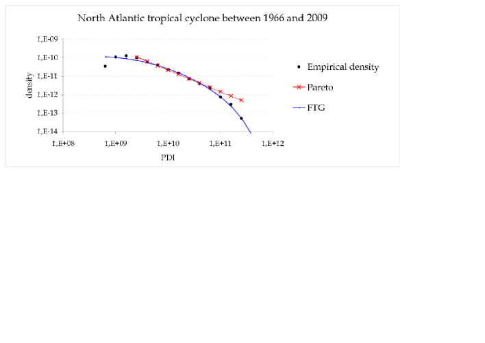
Figure 4.1. FTG distribution fits better than Pareto distribution the tropical cyclones data set, especially in the tail of the observations. The plot is scaled in common logarithm for both axes.

Theorem 1 shows that Pareto distribution is nested in FTG distribution, hence likelihood inference is now available. MLE of parameters and its standard deviations are shown in Table 1 for FTG distribution and Pareto distribution (with two parameters). The values of log-likelihood function are $-667.58$ for FTG case (truncated gamma distribution) and $-680.06$ for the Pareto case.

First of all, the goodness of fit test for Pareto distribution given by Choulakian and Stephens (2001) rejects with p-value less than 0.001 for both statistics, $W^{2}=0.28$ and $A^{2}=2.4$, of the method, but it offers no alternative to the model. Finally, the likelihood ratio test can be used to find a confidence region around the FTG parameters, concluding that the difference between the FTG and the Pareto distribution is highly significant. The $p$-value is $5.8\>10^{-7}$.

	Pareto distribution			FTG distribution
	$\alpha$	$\sigma$	$l$	$\alpha$	$\sigma$	$\rho$	$l$	LRT
MLE	-1.63	2.01	-680.06	0.28	0.09	0.02	-667.58	24.96
s.e.	0.22	0.41		0.15	0.11	0.02

Table 1. MLE for FTG and Pareto distributions for tropical cyclone occurred in the North Atlantic between 1966 and 2009. The data used corresponds to PDI over $3\>10^{9}$, with the origin shifted to zero (units are $10^{10}m^{3}/s^{2}$). This change does not afect the likelihood ratio test, LRT, and the $\alpha$ parameter.

4.2. Analysis of aggregate loss distributions

Financial institutions use internal and external loss data in order to compare several approaches for modelling aggregate loss distributions, associated to quantitative modelling of operational risk, see Dutta and Perry (2006), Degen, et al. (2007) and Moscadelli (2004). The data used for the analysis was collected by several banks participating in the survey to provide individual gross operational losses above a threshold, starting on 2002. The data was grouped by eight standardized business lines and seven event types.

Risk capital is measured as the $99.9\%$ percentile level of the simulated capital estimates for aggregate loss distributions in holding period (1 year). A loss event $L_{i}$ (also known as the loss severity) is an incident for which an entity suffers damages that can be measured with a monetary value. An aggregate loss over a specified period of time can be expressed as the sum

(4.1) $$S=\sum_{i=1}^{N}L_{i}$$

where $N$ is a random variable that represents the frequency of losses that occur over the period. As usual, here it is assumed that the $L_{i}$ are independent and identically distributed, and each $L_{i}$ is independent from $N$, that is Poisson distributed, with parameter $\lambda$.

The data set used here correspond to the $40$ largest losses associated with the business line corporate finance and the event type external fraud, observed over a high threshold, $u$. To maintain confidentiality, the data $\left\{x_{j}\right\}$ has been scaled to threshold zero and mean $100$, according to

$$y_{j}=100\left(\frac{x_{j}-u}{\bar{x}-u}\right)$$

The $40$ exceedances, rounded to two decimal place, were: $0.07$, $0.11$, $0.26$, $0.40$, $0.46$, $0.62$, $0.70$, $0.75$, $0.89$, $1.08$, $1.52$, $1.64$, $1.69$, $2.04$, $2.19$, $2.52$, $2.73$, $3.16$, $3.74$, $4.04$, $4.63$, $5.44$, $5.86$, $6.02$, $10.32$, $19.63$, $29.13$, $30.36$, $30.88$, $35.78$, $40.07$, $46.12$, $137.52$, $237.05$, $311.14$, $314.19$, $396.29$, $552.48$, $864.88$, $891.62$.

Aggregate losses are determined mainly by the extreme values of loss events distribution. In this case, risk capital depends on $40$ exceedances, but, to calculate the $99.9\%$ quantile, a model is required. Under the PoT approach extreme values are modelled with Pareto distribution, see Degen, et al. (2007) and Moscadelli (2004). Pickands-Balkema-DeHaan theorem justifies the approach, see McNeil, et al. (2005). However, this approach may result in unrealistic capital estimates, especially when the fitted Pareto distribution has infinite expectation.

Since the data set has only exceedances over a threshold, the PoT method is the appropriate way. When all losses are recorded, Dutta and Perry (2006) use a four-parameter distribution, called g-and-h, to model the data. If we focus on extreme events of financial assets returns, both upside and downside, standard methodologies also include the classical Student’s t and stable Paretian distributions, see Rachev, et al. (2010).

	Pareto distribution			FTG distribution
	$\alpha$	$\sigma$	$l$	$\alpha$	$\sigma$	$\rho$	$l$	LRT
MLE	-0,45	1,38	-174,44	-0,20	0.65	4.3E-4	-172,37	4,14
s.e.	0.10	0.73		0.16	0.59	6.2E-4

Table 2. MLE for FTG and Pareto distributions of losses by external fraud. FTG distribution is a better model than Pareto distribution, from likelihood ratio test.

Table 2 gives the MLE of parameters for Pareto and FTG distributions, as well as its standard deviations and log-likelihood function, for the last data set. First of all we observe that for Pareto distribution the parameter is in the range $0<\left(-\alpha\right)<1$, that is, a distribution with infinite expectation. This can not be rejected with the goodness of fit test for Pareto distribution given by Choulakian and Stephens (2001), since the parameter is outside the range of parameters provided by their tables. However, Pareto distribution is nested in FTG distribution (Theorem 1) and likelihood ratio test is $4.142$, with p-value $0.042$. Hence, FTG distribution is a more likelihood model for the data set, since Pareto distribution is outside of a $95\%$ confidence region for FTG distribution parameters.

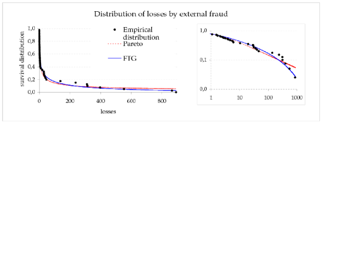
Figure 4.2. The FTG and the Pareto distributions fit the empirical survival function in a similar way in the range of the observed sample. However, the estimated high quantiles differ greatly.The left shows survival distributiona and the picture in the right shows the same plot in common logarithm for the tail of the functions.

Figure 4.2 shows the empirical survival (or reliability) function and its fit given by Pareto and FTG distributions. The probability to exceed the maximum of the sample is estimated at $5,52\%$ for the Pareto distribution and $2.65\%$ for the FTG distribution, this difference does not seem essential. However, the estimation of high quantiles heavily depends on the model. The $0.999$ quantile is $6.95\times 10^{6}$ for the Pareto distribution and $3.93\times 10^{3}$ for the FTG distribution. Moreover, the difference is even greater to calculate the expected tail loss over this quantile, that is the expected value of a loss if a tail event does occur; it is $12970.6$ for the FTG distribution, since (3.2), and infinite for the Pareto distribution. Note that these quantities are measured in a monetary unit (as dollars) to calculate risk capital, hence a factor of $10^{3}$ is really important.

	Pareto distribution			FTG distribution
sample	$\alpha$	$\sigma$	Risk capital	$\alpha$	$\log\theta$	$\log\rho$	Risk capital
1	-0,310	0,367	2,47E+13	-0,038	-7,093	-9,250	10832,98
2	-0,373	1,122	3,50E+11	0,003	-6,771	-8,251	9292,72
3	-0,410	1,719	5,36E+10	-0,106	-7,341	-7,792	13407,05
4	-0,423	1,351	1,87E+10	-0,057	-6,543	-7,460	6934,26
5	-0,441	2,195	1,23E+10	-0,006	-6,520	-7,217	7603,78
6	-0,460	1,205	2,63E+09	-0,298	-8,039	-8,287	16860,11
7	-0,486	1,097	6,78E+08	-0,276	-7,313	-7,828	8921,12
8	-0,538	1,769	1,78E+08	-0,360	-7,613	-7,444	10997,30
9	-0,612	3,923	3,86E+07	-0,257	-6,723	-6,141	6503,94
10	-0,763	3,916	1,66E+06	-0,371	-6,113	-5,461	3276,98
original	-0,448	1,382	5,78E+09	-0,197	-7,325	-7,754	10820,37

Table 3. Parameter estimates and the risk capital from the Pareto distribution and the FTG distribution for 10 bootstrap samples and the original data set.

Risk capital has been calculated as $0.999$ quantile of the aggregate losses, computed from (4.1), by simulating $10^{5}$ times $N$ loss events, where $N$ is Poisson distributed with parameter $\lambda=20$ and the loss events, $L_{i}$, are simulated from the fitted Pareto and FTG distributions. Using the FTG distribution the risk capital is $10820.4$, using Pareto distribution is $5.78\times 10^{9}$. If our data were in thousands of dollars (probably is greater) the Pareto estimation of risk capital for a bank is about the same order as the USA gross domestic product (that is unrealistic), see the last file in Table 3.

In order to see the sample dependence of the risk capital estimate, we generated several bootstrap samples of the same size as the original data set. It is observed immediately, with a small number of samples, the instability of the risk capital estimates obtained with the Pareto distribution. However, the estimates obtained with FTG distribution are much more stable.

Table 3 reports the parameter estimates and the risk capital from the Pareto distribution and the FTG distribution for 10 bootstrap samples and for the original data set. In all cases risk capital has been calculated in the same way. Samples were selected from 100 bootstrap samples, ordered by the parameter $\alpha$, choosing one out of 10, for more diversity. Note that only sample-2 corresponds to the truncated gamma distribution (2.5) and their behaviour is not different from the rest. The most prominent fact is that, in addition to the unrealistic risk capital estimation with Pareto distribution, its estimation is highly unstable, with a factor of $10^{7}$.

We must remember that just as the extreme levels of energy for the tropical cyclones are affected by the limits of the Earth, the economy is also finite. Hence, FTG distribution can be a valuable alternative to Pareto distribution on operational risk.

5. Bibliography

1. Abramowitz, M. and Stegun, I. A. (1972). Handbook of Mathematical Functions with Formulas, Graphs, and Mathematical Tables. New York: Dover.

2. Akinsete, A., Famoye, F and Lee, C. (2008) The beta-Pareto distribution. Statistics, 42, 547 - 563.

3. Arnold, B. C. (1983). Pareto Distributions. Fairland, Maryland: Interna- tional Cooperative Publishing House.

4. Balkema, A., and de Haan, L. (1974). Residual life time at great age. Annals of Probability, 2, 792–804.

5. Barndorff-Nielsen, O. and Cox, D. (1994) Inference and asymptotics. Monographs on Statistics and Applied Probability, 52. Chapman & Hall, London.

6. Barndorff-Nielsen, O. (1978). Information and exponential families in statistical theory. Wiley Series in Probability and Mathematical Statistics. Chichester: John Wiley & Sons.

7. Brown, L. (1986). Fundamentals of statistical exponential families with applications in statistical decision theory. Lecture Notes Monograph Series, 9. Hayward, CA: Institute of Mathematical Statistics.

8. Chapman, D. G. (1956). Estimating the Parameters of a Truncated Gamma Distribution. Ann. Math. Statist., 27, 498-506.

9. Choulakian, V., and Stephens, M. A. (2001). Goodness-of-Fit for the Generalized Pareto Distribution. Technometrics, 43, 478 - 484.

10. Clauset, A., Shalizi, C. R. and Newman, M. E. J. (2009). Power- law Distributions in Empirical Data. SIAM Review, 51, 661 - 703.

11. Coles. S. and Sparks (2006). Extreme value methods for modelling historical series of large volcanic magnitudes. Statistics in Volcanology, Spec. Publ. of the Int. Assoc. of Volcanol. and Chem. of the Earths Inter. Ch. 5.

12. Corral, A., Osso, A. and Llebot, J.E. (2010). Scaling of tropical-cyclone dissipation. Nature Physics, 6, 693 - 696.

13. Davis, H. T. and Michael L. F. (1979). The Generalized Pareto Law as a Model for Progressively Censored Survival Data. Biometrika, 66, 299 - 306.

14. Degen, M., Embrechts, P. and Lambrigger, D. (2007). The quantitative modeling of operational risk: between g-and-h and EVT. Astin Bulletin, 37, 265-291.

15. Den Broeder, G. G. (1955) On parameter estimation for truncated Pearson type III distributions. Ann. Math. Statist, 26, 659 - 663.

16. Devroye, L. (1986). Non-Uniform Random Variate Generation. Springer-Verlag, New York.

17. Dixit, U. J. and Phal, K. D. (2005). Estimating scale parameter of a truncated gamma distribution. Soochwon Journal of Mathematics, 31, 515-523.

18. Dutta, K. and Perry, J. (2006). A Tale of Tails: An Empirical Analysis of Loss Distribution Models for Estimating Operational Risk Capital. Federal Reserve Bank of Boston. Working Paper 06-13.

19. Embrechts, P. Klüppelberg, C. and Mikosch, T. (1997). Modelling Extremal Events for Insurance and Finance. Springer-Verlag, Berlin.

20. Fisher, R. A. (1922). On the mathematical fundations of theoretical statistics. Philos. Trans. Roy. Soc. London, Ser. A, 222, 309 - 368.

21. Furlan, C. (2010). Extreme value methods for modelling historical series of large volcanic magnitudes. Statistical Modelling, 10, 113 - 132.

22. Harter, H. L. (1967). Maximum-likelihood estimation of the parameters of a four-parameter generalized gamma populaton from complete and censored samples. Technometrics, 9, 159 - 165.

23. Hegde, L. M. and Dahiya, R. C. (1989). Estimation of the parameters of a truncated gamma distribution. Communications in Statistics: Theory and Methods, 18, 561 - 577.

24. Letac, G. (1992). Lectures on natural exponential families and their variance functions. Monografias de Matemática, 50, IMPA, Rio de Janeiro.

25. McNeil, A. J., Frey, R. and Embrechts P. (2005). Quantitative Risk Management: Concepts, Techniques and Tools. Princeton University Press.

26. Moscadelli, M. (2004). The modelling of operational risk: experience with the analysis of the data collected by the Basel Committee. Economic working papers, 517, Bank of Italy, Economic Research Department.

27. Philippe, A. (1997). Simulation of right and left truncated gamma distributions by mixtures. Statistics and Computing, 7, 173 - 181.

28. Pickands, J. (1975). Statistical inference using extreme order statistics. Annals of Statistics, 3, 119–131.

29. R Development Core Team (2010). R: A Language and Environment for Statistical Computing. R Foundation for Statistical Computing, Vienna, Austria.

30. Rachev, S. T., Racheva-Iotova, B., Stoyanov, S. (2010). Capturing fat tails, in Risk. Risk Management, Derivatives and Regulation, May 2010, 72-77.

31. Sornette, D. (2006). Critical phenomena in natural sciences. Springer Berlin Heidelberg New York.

32. Stacy, E. W. (1962). A generalization of the gamma distribution. Ann. Math. Stat., 33, 1187 - 1192.