Quantification of noise in the bifunctionality-induced post-translational modification

Abstract

We present a generic analytical scheme for the quantification of fluctuations due to bifunctionality-induced signal transduction within the members of bacterial two-component system. The proposed model takes into account post-translational modifications in terms of elementary phosphotransfer kinetics. Sources of fluctuations due to autophosphorylation, kinase and phosphatase activity of the sensor kinase have been considered in the model via Langevin equations, which are then solved within the framework of linear noise approximation. The resultant analytical expression of phosphorylated response regulators are then used to quantify the noise profile of biologically motivated single and branched pathways. Enhancement and reduction of noise in terms of extra phosphate outflux and influx, respectively, have been analyzed for the branched system. Furthermore, role of fluctuations of the network output in the regulation of a promoter with random activation/deactivation dynamics has been analyzed.

I Introduction

The response of living systems to an external stimulus is coordinated by highly specialized signal transduction machinery. In the bacterial kingdom, this is achieved by the well characterized two-component system (TCS) minimally comprised of the membrane bound sensor kinase (SK) and the cytoplasmic response regulator (RR) Appleby et al. (1996); Hoch (2000); Laub and Goulian (2007); Hart and Alon (2013). The machinery of TCS is utilized by the bacteria to process the information of external signal in terms of phosphotransfer kinetics. When applied, an external stimulus causes phosphorylation at the histidine residue of SK which then gets transferred to the cognate (and/or non-cognate) RR at its aspartate domain. The phosphorylated RR then acts as a transcription factor for several downstream genes, as well as for the activation/represion of its own operon. It is now a well established fact that in addition to being a source (kinase), some SK can also act as a sink (phosphatase) while interacting with an RR Hsing et al. (1998); Laub and Goulian (2007); Goldberg et al. (2010); Hart and Alon (2013). Such bifunctional behavior of SK towards RR can altogether build a robust motif in the bacterial signal transduction network West and Stock (2001); Batchelor and Goulian (2003); Shinar et al. (2007); Siryaporn et al. (2010).

The expression of proteins in individual cells is usually driven by the fluctuations present within the cellular environment as well as the fluctuations imposed by the external stimulus Eldar and Elowitz (2010); Elowitz et al. (2002); Munsky et al. (2012); Paulsson (2004); Rosenfeld et al. (2005); Silva-Rocha and de Lorenzo (2010); Thattai and van Oudenaarden (2001). This often leads to variability in the expression level within the context of a single cell Davidson and Surette (2008); Losick and Desplan (2008); Rotem et al. (2010); Sureka et al. (2008). When observed in the bulk, such fluctuations get averaged out over the cellular population. The prevalent fluctuations, whether external or internal, not only effect the dynamics of gene expression, but also play a major role in post-translational modification Jia and Kulkarni (2010); Mehta et al. (2008). In this connection, it is also important to mention the role of cellular fluctuations in the different signal transduction motif that primarily uses phosphotransfer mechanism. Using a push-pull amplifier loop mechanism, theoretical study has been made to analyze the signal transduction within the photoreceptor of retina Detwiler et al. (2000). Theoretical model has been proposed to study the effect of reversibility in the phosphorylation-dephosphorylation cycle that can generate bistable behavior in the presence of noise and can propagate within the signaling cascade Miller and Beard (2008). In the context of robustness in the bacterial chemotaxis, reversibility on a signaling cascade has been shown to exert a stabilizing effect of adaptation through methylation Alon et al. (1999). Correlation between extrinsic and intrinsic noise due to external signal and internal biochemical pathways, respectively, has also been reported to enhance the robustness of zero-order ultrasensitivity Tănase-Nicola et al. (2006).

Post-translational modification in terms of phosphate transfer is important to generate the pool of phosphorylated RR that acts as a transcription factor for several downstream genes. Bifunctionality, on the other hand, plays a crucial role to maintain this pool as the information flows through the phosphotransfer motif. Thus bifunctionality and post-translational modification work hand in hand to maintain the optimal pool of phosphorylated RR. Since this composite functional behavior takes place in a noisy cellular environment, it is worthwhile to investigate the role of cellular noise on the bifunctionality controlled post-translational modification of the components of the well composed TCS signal transduction machinery. The above observations have motivated us to develop a general model to quantify the molecular noise in the bacterial TCS considering both the bifunctional SK and the post-translational modification of RR. The proposed model takes care of the elementary stochastic phosphotransfer kinetics between the two members (SK and RR) of the TCS and gives a prescription to calculate the fluctuations associated with the phosphorylated RR keeping in mind the bifunctional property of the TCS. We further investigate the role of fluctuations of the network output in the regulation of a promoter with random activation/deactivation kinetics.

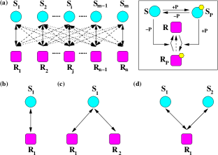
Figure 1: (color online) Wiring diagrams for the proposed post-translational interactions between SK and RR. The cyan circle and magenta square stand for SK and RR, respectively. (a) Generalized $m$:$n$ system with cognate (solid arrow) and non-cognate (dotted, dashed and dotted-dashed arrow) kinase and phosphatase interactions. (b), (c) and (d) are wiring diagrams for 1:1, 1:2 and 2:1 interactions, respectively. The boxed wiring diagram depicts the phosphate addition (+P) and removal (-P) kinetics between a pair of cognate and/or non-cognate SK and RR that ultimately results into phosphorylated RR (magenta square with a yellow hexagon on top). The dotted arrowhead is for auto-dephosphorylation of RR. For simplicity, we do not show the yellow hexagon in (a)-(d).

II The Model

We start by considering a simple system describing post-translational modification driven by phosphotransfer mechanism of a typical TCS, where $m$ numbers of SK interact with $n$ numbers of RR, the ultimate product of which is $R_{p}$, the phosphorylated RR. We call the proposed model as the $m$:$n$ system (Fig. 1a) where each of the SK, RR and their phosphorylated forms are designated as $S$, $R$, $S_{p}$ and $R_{p}$, respectively. The generic model considered here involves single pair interaction (Fig. 1b). In addition, it takes care of branched pathways Laub and Goulian (2007); for example the 1:2 system (Fig. 1c) mimics the one-to-many pathway as observed in chemotaxis system in E. coli, where the SK CheA phosphorylates two RR, CheY and CheB Armitage (1999). Similarly, the 2:1 system (Fig. 1d) follows the kinetics of many-to-one pathway as observed in V. cholerae where the SK LuxS and CqsS phosphorylate the RR LuxO Waters and Bassler (2005).

As mentioned earlier, in typical bacterial TCS, the key steps of phosphotransfer mechanism involve autophosphorylation at SK, transfer of phosphate group from SK to RR, and SK mediated removal of phosphate group from RR (see boxed diagram in Fig. 1). To keep the model simple, we do not consider the synthesis (birth) or degradation (death) of any system component. The interaction we consider here may be of cognate and/or non-cognate type. For $m$:$n$ pair, one can consider the specific interaction between $i$-th SK and $j$-th RR, where $1\leqslant i\leqslant m$ and $1\leqslant j\leqslant n$, to write down the elementary kinetic steps considering the minimal interaction between a specific pair

$$S_{i} \overset{\alpha_{i}}{\underset{\beta_{i}}{\rightleftharpoons}} S_{pi},$$ (1a)

$$S_{pi}+R_{j} \overset{\gamma_{ij}}{\longrightarrow} S_{i}+R_{pj},$$ (1b)

$$S_{i}+R_{pj} \overset{\mu_{ij}}{\longrightarrow} S_{i}+R_{j}.$$ (1c)

$$R_{pj} \overset{\nu_{j}}{\longrightarrow} R_{j}.$$ (1d)

In the above kinetic steps, Eq. (1a) considers autophosphorylation at the histidine residue of the SK. Generally, autophosphorylation takes place under the influence of an external signal Appleby et al. (1996); Hoch (2000); Laub and Goulian (2007) which we consider to be of constant type and is absorbed in the rate constant $\alpha_{i}$. Eqs. (1b-1c) take into account the kinase and phosphatase activity of the SK, respectively, thus considering the bifunctional behavior of the SK. Note that in Eq. (1c), the SK acts as an enzyme to control the dephosphorylation of RR, hence itself remains unchanged Hoch (2000); West and Stock (2001); Laub and Goulian (2007). Eq. (1d) denotes the auto-dephosphorylation of the RR independent of the phosphatase effect of SK on RR Siryaporn et al. (2010).

Due to the inherent noisy nature of the cellular environment, each of the four reactions mentioned above are influenced by fluctuations and in turn affect the copy numbers of each system component. To take this into account, we introduce Langevin noise terms that can influence each of the reactions independently given by Eqs. (1a-1d). The interaction of a single SK with multiple RR or vice versa in presence of fluctuations considered here can be compared with stochastic system-reservoir formalism where a single system interacts with multiple reservoir or vice versa Popov and Hernandez (2007). The stochastic differential equations describing the phosphorylated SK and RR in presence of fluctuations can be written as

$$\frac{dS_{pi}}{dt} = \alpha_{i}(S_{Ti}-S_{pi})-\beta_{i}S_{pi}-\sum_{j=1}^{n}\gamma_{ij}S_{pi}$$ (2a)

$$\times(R_{Tj}-R_{pj})+\xi_{S_{pi}}(t)$$

$$\frac{dR_{pj}}{dt} = \sum_{i=1}^{m}\gamma_{ij}S_{pi}(R_{Tj}-R_{pj})-\sum_{i=1}^{m}[\mu_{ij}$$ (2b)

$$\times(S_{Ti}-S_{Pi})+\nu_{j}]R_{pj}+\xi_{R_{pj}}(t).$$

Here, $S_{Ti}=S_{i}+S_{pi}$ and $R_{Tj}=R_{j}+R_{pj}$ stand for the total amount of $i$-th SK and $j$-th RR, respectively. The additive noise terms $\xi_{S_{pi}}$ and $\xi_{R_{pj}}$ take care of the fluctuations in the copy number of $S_{pi}$ and $R_{pj}$, respectively. Within the framework of linear noise approximation, we define the statistical properties of the Langevin terms obeying the fluctuation-dissipation relation Detwiler et al. (2000); Elf and Ehrenberg (2003); Swain (2004); Bialek and Setayeshgar (2005); Mehta et al. (2008); van Kampen (2005) with zero mean, $\langle\xi_{S_{pi}}(t)\rangle=\langle\xi_{R_{pj}}(t)\rangle=0$ and

$$\langle\xi_{S_{pi}}(t)\xi_{S_{pi}}(t+\tau)\rangle = 2\alpha_{i}(S_{Ti}-\langle S_{pi}\rangle)\delta(\tau),$$

$$\langle\xi_{R_{pj}}(t)\xi_{R_{pj}}(t+\tau)\rangle = 2\sum_{i=1}^{m}\gamma_{ij}\langle S_{pi}\rangle(R_{Tj}-\langle R_{pj}\rangle)\delta(\tau),$$

with $\langle S_{pi}\rangle$ and $\langle R_{pj}\rangle$ being the mean values at the steady state. In addition, the noise terms are correlated Tănase-Nicola et al. (2006); Swain (2004)

$$\langle\xi_{S_{pi}}(t)\xi_{R_{pj}}(t+\tau)\rangle = -\gamma_{ij}\langle S_{pi}\rangle(R_{Tj}-\langle R_{pj}\rangle)\delta(\tau).$$

Since the stochastic Langevin equations (2a-2b) are nonlinear in nature, it is difficult to solve them analytically. To make the solution tractable analytically, we employ linearization of the stochastic equations. The Langevin equation with the linear noise approximation is a valid approach provided the input signal is very small. In addition, such linearization also remains also valid when the time to reach the steady state is longer than the characteristic time scale of the birth and death rate of the system componentsPaulsson (2004); Tănase-Nicola et al. (2006); Hu et al. (2011). Thus, linearizing Eqs. (2a-2b) around the steady state, i.e., $S_{pi}=\langle S_{pi}\rangle+\delta S_{pi}$ and $R_{pj}=\langle R_{pj}\rangle+\delta R_{pj}$, we have

$$\frac{d}{dt}\left(\begin{array}[]{c}\delta S_{pi}\\ \delta R_{pj}\end{array}\right) = \left(\begin{array}[]{cc}-a_{i}&\sum_{j=1}^{n}\gamma_{ij}\langle S_{pi}\rangle\\ \sum_{i=1}^{m}b_{ij}&-c_{j}\end{array}\right)$$ (12)

$$\times\left(\begin{array}[]{c}\delta S_{pi}\\ \delta R_{pj}\end{array}\right)+\left(\begin{array}[]{c}\xi_{S_{pi}}\\ \xi_{R_{pj}}\end{array}\right),$$

where

$$a_{i} = \frac{\alpha_{i}S_{Ti}}{\langle S_{pi}\rangle},b_{ij}=(\mu_{ij}S_{Ti}+\nu_{j})\frac{\langle R_{pj}\rangle}{\langle S_{pi}\rangle},$$

$$c_{j} = \sum_{i=1}^{m}\frac{[\mu_{ij}(S_{Ti}-\langle S_{pi}\rangle)+\nu_{j}]R_{Tj}}{R_{Tj}-\langle R_{pj}\rangle}.$$

Solving Eq. (12) and performing Fourier transformation $\delta\tilde{X}(\omega)={\int_{-\infty}^{\infty}}\delta X(t)e^{-i\omega t}dt$ on the resultant solution, we have in matrix notation, the generalized solution for both $\delta\tilde{S}_{p}(\omega)$ and $\delta\tilde{R}_{p}(\omega)$,

$$\boldsymbol{\delta}{\mathbf{\tilde{S}_{p}}(\omega)} = \mathbf{A}^{-1}\left(\mathbf{\langle S_{pK}\rangle}\boldsymbol{\delta}\mathbf{\tilde{R}_{p}}(\omega)+\boldsymbol{\tilde{\xi}_{S_{p}}}(\omega)\right),$$ (13a)

$$\boldsymbol{\delta}\mathbf{\tilde{R}_{p}(\omega)} = \mathbf{P^{-1}}\left(\mathbf{B}^{\mathrm{T}}\mathbf{A}^{-1}\boldsymbol{\tilde{\xi}}(\omega)+\boldsymbol{\tilde{\xi}_{R_{p}}}(\omega)\right),$$ (13b)

where $\mathbf{P}=\mathbf{C}-\mathbf{B}^{\mathrm{T}}\mathbf{A}^{-1}\mathbf{\langle S_{pK}\rangle}$. In the above expressions (13a-13b), $\boldsymbol{\delta}\mathbf{\tilde{S}_{p}}$ and $\boldsymbol{\delta}\mathbf{\tilde{R}_{p}}$ are $m\times 1$ and $n\times 1$ dimensional column vectors with elements ${\delta}{\tilde{S}_{pi}}$ and ${\delta}{\tilde{R}_{pj}}$, respectively. Likewise, $\boldsymbol{\tilde{\xi}_{S_{p}}}$ and $\boldsymbol{\tilde{\xi}_{R_{p}}}$ are $m\times 1$ and $n\times 1$ column vectors with elements $\tilde{\xi}_{S_{pi}}$ and $\tilde{\xi}_{R_{pj}}$, respectively. ${\mathbf{A}}$ and ${\mathbf{C}}$ are diagonal matrix of order $m\times m$ and $n\times n$ with elements $(i\omega+a_{i})$ and $(i\omega+c_{j})$, respectively. Additionally, $\mathbf{\langle S_{pK}\rangle}$ and $\mathbf{B}$ are matrix of order $m\times n$ with elements $\langle S_{pi}\rangle\gamma_{ij}$ and $b_{ij}$, respectively.

III Results and Discussion

Since we are interested in the effect of noise on phosphorylated RR, $R_{p}$, which acts as transcription factor for one or more genes including the gene that encodes SK and RR, we now focus on the solution of Eq. (13b) only. From the structure of Eq. (13b), it is clear that the dynamics of $R_{p}$ is now decoupled from $S_{p}$. To understand the role of fluctuations in phosphotransfer processes, we define noise at steady state,

$$\eta_{R_{P}}=\sigma_{R_{p}}/\langle R_{p}\rangle,$$

where $\sigma_{R_{p}}$ is the standard deviation of $R_{p}$ (see Fig. 2). It is important to mention that at times fluctuations in the biological systems are quantified using Fano factor, $\sigma_{R_{p}}^{2}/\langle R_{p}\rangle$, where $\sigma_{R_{p}}^{2}$ is the variance of $R_{p}$ (see Fig. 3). Note that in the rest of the discussion we have analyzed our results in terms of steady state noise $\eta_{R_{P}}$ only.

While calculating the noise for the three different systems (1:1, 1:2 and 2:1) mentioned in Fig. 1, we only focus on the noise level of $R_{p1}$, the phosphorylated form of $R_{1}$. Noise generated due to other interactions ($S_{1}$ and $R_{2}$, and $S_{2}$ and $R_{1}$) are considered to add extra layers of information on the noise profile of $R_{p1}$. During the calculation of noise and power spectra we have considered $\gamma_{ij}\approx\mu_{ij}\approx\kappa_{ij}$ $(i,j=1,2)$ for simplicity in the strong limit of protein-protein interaction between SK and RR Siryaporn et al. (2010). It is important to note that while interacting with its partner, an SK shows both monofunctional and bifunctional behavior for $\nu_{j}>\kappa_{ij}$ and $\nu_{j}<\kappa_{ij}$, respectively. At $\nu_{j}\approx\kappa_{ij}$ (cross over regime), the system makes a transition from mono- to bifunctional domain.

Figure 2: Plot of noise, steady state protein level, time series and power spectra for 1:1 system. (a) Noise $\eta_{R_{p1}}$ as a function of $\log_{10}\kappa_{11}$. The noise profile has been shown to contain three different regions, viz monofunctional region ($\kappa_{11}<\nu_{1}$), crossover region ($\kappa_{11}\approx\nu_{1}$) and bifunctional region ($\kappa_{11}>\nu_{1}$). In the absence of auto-dephosphorylation kinetics (Eq. (1d)), only the bifunctional domain exists, whereas in the absence of phosphatase kinetics (Eq. (1c)), only the monofunctional domain becomes prevalent. The open circles are due to Gillespie simulation Gillespie (1976, 1977). For comparison of the noise profile with the Fano factor, see Fig. 3. (b) Steady state $R_{p1}$ as a function of $\log_{10}\kappa_{11}$. (c)-(e) Time series of $R_{p1}$ for low ($\kappa_{11}=10^{-5}$), intermediate ($\kappa_{11}=10^{-2}$) and high ($\kappa_{11}=1$) values of $\kappa_{11}$, respectively, generated using Gillespie algorithm Gillespie (1976, 1977). Note that in (d) the ordinate does not start from zero. (f) Normalized power spectra for low (solid line), intermediate (dashed line) and high (dotted line) values of $\kappa_{11}$. In all the cases, $\alpha_{1}/\beta_{1}=5$, $\nu_{1}=0.01$ and $S_{T1}=R_{T1}=20$.

In Fig. 2a noise profile of $R_{p1}$ has been shown in a semilog plot. For 1:1 system, at a low value of $\kappa_{11}$, noise has a nonzero value which goes down as $\kappa_{11}$ value increases. As $\kappa_{11}$ value increases further, noise increases and reaches a high value. As evident from the definition, noise is inversely proportional to the population of steady state $R_{p1}$. To check the role of $\langle R_{p1}\rangle$ on steady state noise, we have calculated $\langle R_{p1}\rangle$ as a function of $\log_{10}\kappa_{11}$ (Fig. 2b) from which it is evident that the protein profile develops exactly in a way opposite to the noise profile and imparts an inverse effect on the noise development. For a low value of $\kappa_{11}$, the auto-dephosphorylation $\nu_{1}$ dominates over the phosphatase activity of SK on RR ($\kappa_{11}<\nu_{1}$). In this regime, the sensor shows monofunctional activity by acting as a kinase only, which is still lower than $\nu_{1}$. This effectively reduces the $R_{p1}$ level (Fig. 2c) and increases the noise of the system. In the limit $\kappa_{11}\approx\nu_{1}$ (vertical dotted line in Fig. 2a), $R_{p1}$ level reaches its maximum (Fig. 2b and Fig. 2d) while reducing the noise. When $\kappa_{11}$ exceeds $\nu_{1}$ ($\kappa_{11}>\nu_{1}$), the phosphatase activity of SK starts to show up in addition to its kinase activity. In this regime, the bifunctional property of SK comes into play reducing the copy of $R_{p1}$ (Fig. 2e) henceforth increasing the noise of the system. To compare the noise profile of $R_{p1}$ given in Fig. 2a with the Fano factor ($\sigma_{R_{p1}}^{2}/\langle R_{p1}\rangle$) of the same quantity, we have shown the dependence of Fano factor on $\kappa_{11}$ in Fig. 3. To understand how the system relaxes under the influence of the protein-protein interaction, we calculate the power spectra $S(\omega)=\langle\delta\tilde{R}_{p1}(\omega)\delta\tilde{R}_{p1}(\omega^{\prime})\rangle$ (Fig. 2f). The resultant spectral lines are plotted for low, intermediate and high $\kappa_{11}$ values. As expected, the power spectra relaxes faster for a low $\kappa_{11}$ value compared to an intermediate $\kappa_{11}$ value which again relaxes faster compared to a high $\kappa_{11}$ value. For a low value of $\kappa_{11}$, the conversion of $R$ into $R_{p}$ is a slow process and hence fast fluctuations in the copy number have minimal effect on the power spectrum. As $\kappa_{11}$ value increases, the conversion rate increases and thus gets affected by the noise in the copy number which results into slower relaxation.

Figure 3: Plot of Fano factor as a function of $\log_{10}\kappa_{11}$ for 1:1 system. The solid line is due to the theoretical calculation and the open circles are generated using Gillespie simulation Gillespie (1976, 1977). The values of other parameters are same as in Fig. 2.

In Figs. 4a-4c, we show the noise, $\eta_{R_{p1}}$ for 1:2 and 2:1 system as a function of $\kappa_{11}$ in a semilog plot. For comparison, we refer to noise profile of 1:1 system shown in Fig. 2a. In 1:2 system, a single SK, $S_{1}$ interacts with two RRs, $R_{1}$ and $R_{2}$, with its bifunctional properties acting on both the RRs. In Fig. 4a, we show the noise generated for $R_{p1}$ while considering the kinase and phosphatase rates ($\gamma_{12}\approx\mu_{12}\approx\kappa_{12}$) between $S_{1}$ and $R_{2}$ to be low ($\kappa_{12}=10^{-5}$), intermediate ($\kappa_{12}=10^{-2}$) and high ($\kappa_{12}=1$). For low and intermediate $\kappa_{12}$ values, the noise profile looks almost that of like 1:1 system as $\kappa_{11}$ is varied. This happens as the interaction between $S_{1}$ and $R_{2}$ adds a weak layer of information on $R_{1}$ due to monofunctional property of $S_{1}$ on $R_{2}$ ($\nu_{2}\geqslant\kappa_{12}$). On the other hand, for a high $\kappa_{12}$ value, a huge amplification of noise occurs (the dotted line in Fig. 4a). In this domain, as $\nu_{2}<\kappa_{12}$, SK starts to show its bifunctional property and is more active in its interaction with $R_{2}$, rather than with $R_{1}$. Such active interaction between $S_{1}$ and $R_{2}$ adds an extra layer of outflux of phosphate group from $R_{1}$ (the dotted line in Fig. 4b) thus leading to a low level of $\langle R_{p1}\rangle$ and an enhancement of noise.

Figure 4: Plot of noise and steady state protein level for branched (1:2 and 2:1) pathways. (a,c) Noise profile for 1:2 and 2:1 system, respectively, as a function of $\log_{10}\kappa_{11}$. The solid, dashed and dotted lines are for low ($10^{-5}$), intermediate ($10^{-2}$) and high ($1$) values of $\kappa_{12}$ (for 1:2) and $\kappa_{21}$ (for 2:1). (b,d) Steady state level of $R_{p1}$ for the same values of $\kappa_{12}$ and $\kappa_{21}$ as in (a,c). For all the cases, $\alpha_{i}/\beta_{i}=5$, $\nu_{j}=0.01$ and $S_{Ti}=R_{Tj}=20$.

In 2:1 system, a single RR, $R_{1}$ interacts with two SKs, $S_{1}$ and $S_{2}$. In Fig. 4c, we show the noise generated for $R_{p1}$ while taking into account the kinase and phosphatase rates ($\gamma_{21}\approx\mu_{21}\approx\kappa_{21}$) between $S_{2}$ and $R_{1}$ to be low ($\kappa_{21}=10^{-5}$), intermediate ($\kappa_{21}=10^{-2}$) and high ($\kappa_{21}=1$). For low value of $\kappa_{21}$, the noise profile is similar to that of a 1:1 system as $\kappa_{11}$ is increased. Although in this domain $S_{2}$ acts as kinase only, it provides a low level of input on $R_{1}$ as $\nu_{1}>\kappa_{21}$. Interesting behavior emerges as $\kappa_{21}$ takes an intermediate and high values. In the intermediate domain, maximal level of $\langle R_{p1}\rangle$ is produced due to extra influx of phosphate group. This large influx due to $\kappa_{21}$ can overpower the low kinase effect of $\kappa_{11}$, and hence increase the steady state level of $R_{p1}$ as a effect of which the noise level attains a minimum value. For high $\kappa_{21}$, $\nu_{1}<\kappa_{21}$ where $S_{2}$ starts to show its bifunctional property via phosphate input and removal. This helps the composite system to maintain a high value of noise for a wide range. Note that, compared to the low and intermediate domain, the protein level in this region goes down drastically due to strong phosphatase activity of $S_{2}$ on $R_{1}$. It is interesting to note that for intermediate and high $\kappa_{21}$ value, the composite system loses it monofunctional behavior almost completely (Fig. 4d).

To check the effect of the network in the regulation of the downstream promoter activity, one needs to consider the fluctuations in $R_{p}$ level as extrinsic noise while the promoter activation/inactivation is governed by the intrinsic molecular fluctuations Hu et al. (2011, 2012). The time scale for the relaxation of the network is given by $\tau_{in}$ where $\tau_{in}=c_{j}^{-1}$. The promoter switching kinetics, driven by output of the network (i.e., $R_{p}$), can be modeled as

$$Off\overset{k_{on}R_{p}(t)}{\underset{k_{off}}{\rightleftharpoons}}On.$$ (14)

Now following Ref. Hu et al., 2012, we associate a variable $D$ with the switching process of the promoter, where $D$ takes the value 0 and 1 for the off and the on state of the promoter, respectively. The stochastic Langevin equation associated with $D$ can be written as Mehta et al. (2008)

$$\frac{dD}{dt}=k_{on}R_{p}(1-D)-k_{off}D+\xi_{D}(t),$$ (15)

where $\langle\xi_{D}(t)\rangle=0$ and

$$\langle\xi_{D}(t)\xi_{D}(t+\tau)\rangle=2k_{off}\langle D\rangle\delta(\tau),$$

with steady state value $\langle D\rangle=\langle R_{p}\rangle/(\langle R_{p}\rangle+K_{d})$ and $K_{d}=k_{off}/k_{on}$. The Langevin equation is simply a noisy version of the deterministic chemical kinetics, which on the noise averaged level would yield the average value of the variable $D$ for the on state of the promoter. Following Eq. (15), we associate a time scale for the promoter switching kinetics $\tau_{out}$, where $\tau_{out}=(k_{on}\langle R_{p}\rangle+k_{off})^{-1}$, a characteristics of noiseless input model. Now linearizing Eq. (15) and performing Fourier transformation of the linearized equation, one arrives at Mehta et al. (2008)

$$\delta\tilde{D}(\omega)=\frac{\tilde{\xi}_{D}(\omega)}{i\omega+\tau_{out}^{-1}}+\frac{k_{on}(1-\langle D\rangle)}{i\omega+\tau_{out}^{-1}}\delta\tilde{R}_{p}(\omega).$$ (16)

Note that the first term on the right hand side of Eq. (16) arises due to the noiseless input model (mean field input of $R_{p}$) and incorporates only the fluctuations in the promoter switching kinetics, whereas the second term appears via the noisy input due to the fluctuations in the $R_{p}$ level. We now define the total variance associated with $D$ at steady state for the noisy input model as

$$\sigma^{2}_{D}=\frac{K_{d}\langle R_{p}\rangle}{(\langle R_{p}\rangle+K_{d})^{2}}+\frac{K_{d}k_{off}}{(\langle R_{p}\rangle+K_{d})^{3}}\sigma^{2}_{R_{p}},$$ (17)

where $\sigma^{2}_{D}=(1/2\pi)\int d\omega\langle|\delta\tilde{D}(\omega)|^{2}\rangle$. Here, the first and the second term on the right hand side of Eq. (17) arises due to noiseless input model and fluctuations in the $R_{p}$ level, respectively. At this point, it is important to mention that an almost similar expression for the variance $\sigma^{2}_{D}$ was obtained by Hu et al in their recent work on the role of input noise in genetic switch (see Eq. (14) of Ref. Hu et al., 2012). To be explicit, Ref. Hu et al., 2012 shows that for a noisy input model, the value of $\langle D\rangle$ itself changes in comparison to the noiseless input model (constant $R_{p}$) which eventually changes the variance. Thus, considering the kinetics of promoter switching as a simple binary process in the presence of noisy input one arrives at the aforesaid expression of $\sigma^{2}_{D}$ which incorporates the essential features of noiseless input model as well as the fluctuations in the $R_{p}$ level (via $\delta\tilde{R}_{p}(\omega)$, see Eq. (13b)). This result suggests that the variance due to the noiseless input model gets modified in the presence of a noisy input and is in agreement with the result shown in Ref. Hu et al., 2012.

To check how the time scale of the noisy input (fluctuations in the $R_{p}$ level) affects the promoter switching kinetics, we define noise associated with the promoter switching at steady state for the noisy input model as $\eta_{D}=\sigma_{D}/\langle D\rangle$, where

$$\eta_{D}=\left[\frac{K_{d}}{\langle R_{p}\rangle}+\frac{K_{d}k_{off}}{(\langle R_{p}\rangle+K_{d})}\eta^{2}_{R_{p}}\right]^{1/2}.$$ (18)

Figure 5: (a-c) Plot of $\eta_{D}$ as a function of promoter switching time scale $\tau_{out}$, for $\kappa_{11}=4\times 10^{-4},10^{-2}$ and 0.4, respectively. The solid (with open squares) and the dashed (with open circles) lines are for noiseless and noisy input model, respectively. (d) Contributions due to fluctuations in the $R_{p}$ level. The solid (with open squares), dashed (with open circles) and dotted (with open triangles) lines are due to $\kappa_{11}=4\times 10^{-4},10^{-2}$ and 0.4, respectively. In all the panels, lines are drawn using Eq. (18) and the symbols are generated using Gillespie simulation Gillespie (1976, 1977).

The first and the second term on the right hand side of Eq. (18) is due to the noiseless input model and the fluctuations in the $R_{p}$ level, respectively, as suggested by Eq. (17). In Fig. 5, we show the dependence of $\eta_{D}$ on the promoter switching time scale $\tau_{out}$ for 1:1 system for low, intermediate and high values of $\kappa_{11}$. The three values of $\kappa_{11}$ have been chosen from the monofunctional, cross-over and bifunctional regime, respectively, of the TCS signal transduction motif (see Fig. 2a). Fig. 5 suggests that for low and high values of $\kappa_{11}$, the fluctuations associated with the promoter switching kinetics due to noisy input model are higher (dashed line with open circles in Figs. 5a,5c) as the fluctuations due to $R_{p}$ level ($\eta_{R_{p}}$, see also Fig. 2a) at these parameter regimes are high. However, for the intermediate $\kappa_{11}$ value, the fluctuations are minimum (dashed line with open circles in Fig. 5b) as the TCS maintains a minimum noise level at this $\kappa_{11}$ value. For reference, we show the fluctuations associated with the noiseless input model in Figs. 5a-5c (solid line with open squares) which clearly explains enhancement of noise for the noisy input model due to fluctuations in the $R_{p}$ level (Fig. 5d).

Fig. 5d shows that as $\tau_{out}$ increases, the contribution due to the $R_{p}$ level fluctuations in the promoter switching kinetics decreases, which is a general trend for all the $\kappa_{11}$ values. In the limit of fast promoter switching rate (low $\tau_{out}$) compared to the time scale of the $R_{p}$ level fluctuations ($\tau_{in}$), $\tau_{out}\ll\tau_{in}$. At this limit, the contribution due to noisy input is high and the output of the network (TCS) affects the promoter switching kinetics maximally. On the other hand, when the promoter switching rate is slow (high $\tau_{out}$) compared to the variation of network output time scale such that $\tau_{out}\gg\tau_{in}$, the network output exerts a mean field effect on the promoter switching rate. At this limit contribution due to the noisy input reduces drastically (second term on the right hand side of Eq. (18)) and one recovers the behavior of the noiseless input model.

IV Conclusion

To conclude, we have provided a generic description for the calculation of noise due to post-translational modification in the bacterial TCS. From exact analytical calculation within the purview of linear noise approximation, it is possible to quantify the steady state noise for the single pair and for the branched pathways. For the single pair system, our analysis shows the effect of bifunctionality of SK on noise generation and can differentiate the mono- and the bifunctional domain in the noise profile. The calculation for the branched pathways shows enhancement and reduction of noise for the composite system in terms of extra phosphate outflux and influx, respectively. Our analysis suggests that in one to many system as in the chemotaxis pathway of E. coli, enhancement of fluctuations happens due to extra outflux of phosphate group within the members of TCS. On the other hand, for many to one system mimicking the quorum sensing network of V. cholerae, an optimal level of noise can be maintained via extra influx of phosphate group. To maintain such low noise activity, SK of V. cholerae phosphotransfer circuit might prefer to operate in the cross over domain.

The motif of TCS in the bacterial kingdom reliably transmits the information of the changes made in the extracellular environment within the cell. This happens via the formation of the pool of $R_{p}$ which acts as a transcription factor for several genes including the genes encoding the TCS. The molecular fluctuations due to the post-translational modification during the formation of $R_{p}$ play an important role in the fluctuations of the gene expression mechanism. While acting as a transcription factor the noise due to $R_{p}$ level fluctuations acts as a noisy input in the gene expression mechanism. On ther hand, the promoter activation/inactivation mechanism is characterized by the intrinsic molecular fluctuations. Keeping this in mind, we have investigated the possible role of the network output on the promoter switching kinetics. The fluctuations associated with the promoter switching mechanism have been quantified by the total noise at steady state associated with the active state of the promoter. Our analysis suggests that the total noise $\eta_{D}$ at steady state is comprised of two parts; the first part arises due to the noiseless input model while the second part is due to the noisy contribution of the TCS network output. If the fluctuations in the $R_{p}$ level occur on a faster time scale, it hardly affects the process of transcription as the DNA promoter activation/inactivation mechanism gets weakly affected. In such a situation, the transcription factor $R_{p}$ exerts a mean field effect in the process of transcription and fluctuations in the promoter switching kinetics are predominantly governed by the intrinsic molecular noise, a typical characteristics of the noiseless input model. On the other hand, when the time scale of $R_{p}$ fluctuations is slower/comparable than the promoter switching rate, it exerts a considerable effect on the promoter switching mechanism. In other words, when the fluctuations in the $R_{p}$ level maintain an optimal level and is comparable with the time scale of the DNA promoter switching rate, the latter gets highly affected by the changes made in the extra-cellular environment which has been reliably transmitted through the TCS. The formalism we present in this work gives an idea of the optimal level of fluctuations within the TCS which is necessary for reliable transmission of signal to control the regulation of biochemical switch present within the bacterial cell.