Complete analysis and generation of hyperentangled Greenberger-Horne-Zeilinger state for photons using quantum-dot spins in optical microcavities

Abstract

We propose a scheme for the complete differentiation of 64 three-photon hyperentangled GHZ states in both polarization and spatial-mode degrees of freedoms using the quantum-dot cavity system. The three-photon hyperentangled-GHZ-state-analysis scheme can also be used to generate 3-photon hyperentangled GHZ states. This proposed hyperentangled analysis and generation device can serve as crucial components of the high-capacity, long-distance quantum communication. We use quantum swapping as an example to show the application of this device in manipulating multiparticle entanglement with polarization and spatial-mode degrees of freedoms. Using numerical calculations, we show that the present scheme may be feasible in strong-coupling regimes with current technologies.

I Introduction

Entangled states play a critical role in quantum information processing, including quantum computation 1 and quantum communication teleporation ; densecoding ; 2 . Compared with two-partite entangled states, which are well understood, the entanglement between three or more particles is more fascinating and interesting. As an extension from the two-qubit Bell-state to a multipartite system, the Greenberger-Horne-Zeilinger (GHZ) state ghz is a maximally entangled state of three or more particles, and it can be generated in different quantum systems. For example, GHZ states can be created from two pairs of entangled photons photonghz and the excitons of coupled quantum dots qdghz . Researchers have also constructed GHZ states nonlocally in distant emitter-cavity systems, such as atom-cavity system atomghz and nitrogen vacancy (N-V) centers-photonic crystal (PC) nano-cavity system nvghz . The GHZ state is one of the most important multiparticle quantum resources because its potential applications in quantum information processing such as quantum teleportation ghztele , entanglement swapping ghzswap , fundamental test of quantum mechanics ghztest and quantum cryptographicdensecoding ; xiayanhgsa . In most of these applications, the efficient measurement and analysis of entangled states are essential and demanding.

The complete and deterministic analysis of the two-qubit and multi-qubit entangled states is required as a vital element for many important applications in quantum communication, such as quantum teleportation teleporation ; teleporation1 ; teleporation2 ; ghztele , quantum dense coding densecoding ; wangcoding , quantum superdense coding superdensecoding , and so on. Many approaches have been investigated for two-qubit and three-qubit entangled analyzers. For example, only with the help of linear optics, the probability for analysis of Bell-states is 50% and the probability for analyzing GHZ states (GSA) is 25% GHZA . However, Hyperentanglement allows the complete analysis of entanglement state becomes possible. Hyperentanglement is the entanglement of photons simultaneously existing in more than one degree of freedom (DOF). In 2003, Walborn et al. HyperentangledBell-stateanalysis2003 proposed a simple linear-optical scheme for the complete Bell-state measurement of photons by using hyperentanglement. In 2006, Carsten Schuck et al. HyperentangledBell-stateanalysis2006 deterministically distinguished all four polarization Bell states of entangled photon pairs with the aid of polarization-time-bin hyperentanglement in an experiment. In 2007, Barbieri et al. HyperentangledBell-stateanalysis2007p-m realized complete and deterministic Bell-state measurement in the experiment using linear optics and two-photon polarization-momentum hyperentanglement. In 2012, Song et al. song proposed a scheme to distinguish eight GHZ states completely using polarization-spatial-mode hyperentanglement with only linear optics.

Aside from the complete analysis of entangled states, other applications of hyperentanglement have been extensively studied because it can improve the channel capacity of long-distance quantum communications and offers significant advantages in quantum communication protocols. For example, hyperentanglement can be used for quantum error-correcting code hyperentanglement-app-error-correctingcode , high-capacity quantum cryptography wangcoding ; hyperentanglement-app-c , quantum repeaters wangtjpra , and deterministic entanglement purification hpur . The 16 hyperentangled two-qubit Bell states shengprainpress and 64 three-qubit GHZ states xiayanhgsa may be completely distinguished with the help of cross-Kerr nonlinearity in the optical single-photon regime. However, due to the weak cross-Kerr nonlinearity, the schemes are currently without technical support 44 ; 45 .

Embedding quantum dots QD (QDs) into solid-state cavities is relatively easy, and the deterministic transfer of quantum information between photons and spins in QDs can be promoted by two typical structures of cavity-QD systems, i.e., the double-sided cavity-QD system and the single-sided cavity-QD system (see in Fig.1). These two spin-cavity systems can be used to produce entangled photon-states, such as the Bell state, the GHZ state, and cluster state7 ; hybrid ; 9 and perform Bell-state 6 ; 13 and hyperentangled Bell-state renoehbsa ; Wangprahbsa analysis. Double-sided-cavity-spin systems have been proven to work like a beam splitter when limited by a weak incoming field beamsplitter in a weak-coupling cavity where the vacuum Rabi frequency is less than the cavity decay rate. Thus, the double-sided cavity-spin unit can be used as a SWAP gate between the polarization DOF and the spatial-mode DOF of photons and records the relationship between the phase information in these DOFs Wangprahbsa . The single-sided cavity-QD unit can be used as a parity checking device that will pick up a phase $\theta$ on the photon if this photon is coupled with the spin in QD, and the $\theta$ is turnable 13 . Because of its high quantum efficiency, single-photon characteristics, and high stability, the spin-photon interface has been widely studied in deterministic optical quantum computing 10 , construction universal gates 6 ; 7 ; 9 , hybrid entanglement generation hybrid , and quantum purification and concentration WANGCHUAN ; wangoe .

In this paper, we take the advantages of these two spin-cavity units and propose a scheme that can be used as a complete three-qubit hyperentangled-GHZ-state analyzer (HGSA). The scheme can be used to generate 3-photon hyperentangled GHZ states and increase the channel capacity of long-distance quantum communication. The proposed HGSA device can be applied in the crucial components of long-distance quantum communication, such as high-capacity teleportation, entanglement swapping, and some important quantum cryptographic schemes xiayanhgsa . As the GHZ state is the extension of two-qubit Bell state to multi-qubit system, this device can also be used to analysis hyperentangled Bell-state photon-pairs. Compared with the previous work renoehbsa ; Wangprahbsa , this scheme has some advantages. First, it is much simpler than those schemes because only two spin-cavity units are employed here, not four or more. Second, it can be generalized to N-photon hyperentangled GHZ states analysis, and the number of the required spin-cavity units will not increase with the number of the photons. Moreover, it can be used to generate hyperentangled GHZ states. With existing experimental data, we demonstrate that the present scheme can work in the strong-coupling regime using current technologies.

II The complete analysis of hyperentangled three-photon GHZ states in two DOFs using quantum-dot spin and optical double-sided microcavity system

In this section, we introduce the principle of the complete analysis of hyperentangled three-photon GHZ state in polarization and the spatial-mode DOFs using quantum-dot spin and optical double-sided microcavity system. A quantum system with three photons hyperentangled in polarization and spatial-mode DOFs has 64 generalized GHZ states that can be expressed as

$$|\varphi^{ABC}\rangle_{PS}=|\Psi_{ABC}\rangle_{P}\otimes|\Phi_{ABC}\rangle_{S}$$ (1)

where subscripts $A$, $B$ and $C$ represent the three photons in the hyperentangled state. The subscript $P$ denotes the polarization DOF of the photons and $|\Psi_{ABC}\rangle_{P}$ is one of the eight Bell states in the polarization DOF, which is expressed as

$$|\Psi^{\pm}_{1}\rangle_{P}=\frac{1}{\sqrt{2}}(|RRR\rangle_{ABC}\pm|LLL\rangle_{ABC}),\;\;|\Psi^{\pm}_{2}\rangle_{P}=\frac{1}{\sqrt{2}}(|RRL\rangle_{ABC}\pm|LLR\rangle_{ABC}),$$

$$|\Psi^{\pm}_{3}\rangle_{P}=\frac{1}{\sqrt{2}}(|RLR\rangle_{ABC}\pm|LRL\rangle_{ABC}),\;\;|\Psi^{\pm}_{4}\rangle_{P}=\frac{1}{\sqrt{2}}(|LRR\rangle_{ABC}\pm|RLL\rangle_{ABC}).$$ (2)

Here, $|L\rangle$ and $|R\rangle$ represent the left and right circular polarizations of photons, respectively. The subscript $S$ denotes the spatial-mode DOF and $|\Phi_{ABC}\rangle_{S}$ is one of the eight Bell states in the spatial-mode DOF, which is expressed as

$$|\Phi^{\pm}_{1}\rangle_{S}=\frac{1}{\sqrt{2}}(|a_{1}b_{1}c_{1}\rangle_{ABC}\pm|a_{2}b_{2}c_{2}\rangle_{ABC}),\;\;|\Phi^{\pm}_{2}\rangle_{S}=\frac{1}{\sqrt{2}}(|a_{1}b_{1}c_{2}\rangle_{ABC}\pm|a_{2}b_{2}c_{1}\rangle_{ABC}),$$

$$|\Phi^{\pm}_{3}\rangle_{S}=\frac{1}{\sqrt{2}}(|a_{1}b_{2}c_{1}\rangle_{ABC}\pm|a_{2}b_{1}c_{2}\rangle_{ABC}),\;\;|\Phi^{\pm}_{4}\rangle_{S}=\frac{1}{\sqrt{2}}(|a_{2}b_{1}c_{1}\rangle_{ABC}\pm|a_{1}b_{2}c_{2}\rangle_{ABC}),$$ (3)

where $i_{1}$ and $i_{2}$ ($i$ is $a,$ $b,$ or $c$) are the different spatial modes for the photon $I$ ($I$ is corresponding photon $A$, $B,$ or $C$). Consider that the three hyperentangled photons $ABC$ is in one of the 64 hyperentangled GHZ states that forms in Eq. (1). The principles of the complete three-photon HGSA is shown in Fig. 2 .

II.1 Measurement of the relation of the phase information between two DOFs by using quantum-dot spin and optical double-sided microcavity system

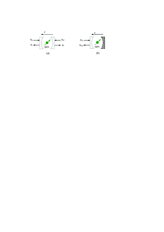
Figure 1: A charged quantum dot inside a double-sided (a) or in a single-sided (b) micropillar cavity. An exciton consisting of two electrons bound to one hole with negative charges can be created by the optical excitation of a photon and an electron-spin.

The first cavity (cavity 1) is a double-sided optical microcavity in which the top and bottom mirrors are both partially reflective, as shown in Fig. 1 (a), and a singly charged QD is embedded in cavity 1. The spin of this QD (spin 1) is initialized in the state $|\Psi^{s}\rangle_{1}=(|\uparrow\rangle+|\downarrow\rangle)_{1}/\sqrt{2}$. Pauli’s exclusion principle illustrates that, the $|\uparrow\rangle$ spin state ($J_{z}=+\frac{1}{2}$) only couples with the $s_{z}=1$ photon, i.e., the $|R^{\uparrow}\rangle$ or $|L^{\downarrow}\rangle$ photon, to the exciton X^- in state $|\uparrow\downarrow\Uparrow\rangle$. When the electron spin is in the spin state $|\downarrow\rangle$ $(J_{z}=-\frac{1}{2})$, it only couples the photon that is in the state $|R^{\downarrow}\rangle$ or $|L^{\uparrow}\rangle(s_{z}=-1)$ to the exciton X^- in state $|\downarrow\uparrow\Downarrow\rangle$. Here, $|\Uparrow\rangle$ and $|\Downarrow\rangle$ represent heavy-hole spin states with $J_{z}=\frac{3}{2}$ and $J_{z}=-\frac{3}{2}$, respectively, and the superscript arrows $\uparrow$ and $\downarrow$ in the photon state indicate the propagation direction along the $z$ axis. For a double-sided cavity, the coupling photon will be reflected by the cavity and the uncoupling photon will pass through the cavity. All reflection and transmission coefficients of this spin-cavity system can be determined by solving the Heisenberg equations of motion for the cavity-field operator ($\hat{a}$) and the exciton $X^{-}$ dipole operator ($\sigma_{-}$) in weak excitation approximation 6 ; 7 ; hybrid ; 9

$$\frac{d\hat{a}}{dt} = -[i(\omega_{c}-\omega)+\kappa+\frac{\kappa_{s}}{2}]\hat{a}-g\sigma_{-}-\sqrt{\kappa}\hat{a}_{in^{\prime}}-\sqrt{\kappa}\hat{a}_{in}+\hat{H},$$

$$\frac{d\sigma_{-}}{dt} = -[i(\omega_{X^{-}}-\omega)+\frac{\gamma}{2}]\sigma_{-}-g\sigma_{z}\hat{a}+\hat{G},$$

$$\;\;\hat{a}_{r}\; = \hat{a}_{in}+\sqrt{\kappa}\hat{a},\;\;\;\hat{a}_{t}\;=\hat{a}_{in^{\prime}}+\sqrt{\kappa}\hat{a},$$ (4)

where $\omega$, $\omega_{c}$, and $\omega_{X^{-}}$ are the frequencies of the photon, the cavity and $X^{-}$ transition, respectively; $g$ represents the coupling constant; $\gamma$ is the exciton dipole decay rate; and $\kappa$ and $\kappa_{s}$ are the cavity decay rate and the leaky rate, respectively. $\hat{H}$ and $\hat{G}$ are the noise operators related to reservoirs. $\hat{a}_{in}$, $\hat{a}_{in^{\prime}}$ and $\hat{a}_{r}$, $\hat{a}_{t}$ are the input and output field operators. For a double-sided optical microcavity system beamsplitter ; hybrid , the reflection $r_{h}$ and transmission $t_{h}$ coefficient in a coupled cavity in the resonant interaction case can be described by

$$r_{h}(\omega) = 1+t_{h}(\omega),$$

$$t_{h}(\omega) = -\frac{\kappa[i(\omega_{X^{-}}-\omega)+\frac{\gamma}{2}]}{[i(\omega_{X^{-}}-\omega)+\frac{\gamma}{2}][i(\omega_{c}-\omega)+\kappa+\frac{\kappa_{s}}{2}]+g^{2}}.$$ (5)

When $g=0$, the reflection $r_{0}$ and transmission $t_{0}$ coefficients in an uncoupled cavity are

$$r_{0}(\omega)=\frac{i(\omega_{0}-\omega)+\frac{\kappa_{s}}{2}}{i(\omega_{c}-\omega)+\kappa+\frac{\kappa_{s}}{2}},\;\;t_{0}(\omega)=\frac{-\kappa}{i(\omega_{0}-\omega)+\kappa+\frac{\kappa_{s}}{2}}.$$ (6)

Thus, when the side leakage and cavity loss ($k_{s}$) can be ignored, in the resonant interaction case, the cold (uncoupled) and hot (coupled) cavities generally have different reflection and transmission coefficients, and the dynamics of the photon and of the spin in the cavity are described as follows:

$$|R^{\uparrow},\uparrow\rangle\rightarrow|L^{\downarrow},\uparrow\rangle,\;\;\;\;|L^{\uparrow},\uparrow\rangle\rightarrow-|L^{\uparrow},\uparrow\rangle,\;\;\;\;|R^{\downarrow},\uparrow\rangle\rightarrow-|R^{\downarrow},\uparrow\rangle,\;\;\;\;|L^{\downarrow},\uparrow\rangle\rightarrow|R^{\uparrow},\uparrow\rangle,$$

$$|R^{\uparrow},\downarrow\rangle\rightarrow-|R^{\uparrow},\downarrow\rangle,\;\;\;\;|L^{\uparrow},\downarrow\rangle\rightarrow|R^{\downarrow},\downarrow\rangle,\;\;\;\;|R^{\downarrow},\downarrow\rangle\rightarrow|L^{\uparrow},\downarrow\rangle,\;\;\;\;|L^{\downarrow},\downarrow\rangle\rightarrow-|L^{\downarrow},\downarrow\rangle.$$ (7)

From the Eq. (7), one can see that for the coupling case, the photon will be reflected by the cavity and the polarized state of the photon will be flipped for the unchanged photon spin $s_{z}$. For the uncoupling case, the photon will only add a $\pi$ phase when it passes through the cavity. The photon polarization and electron spin may become entangled when this spin-cavity unit is used.

Using the spin-cavity unit discussed above, one can record the relation between two DOFs. After the interaction between the spin 1 and photons $ABC$, the state in this two DOFs can be exchanged, and the phase information in this two DOfs will be flipped. First, let photons $A$, $B$, and $C$ successively pass through the cavity 1 from the left input-port. A time interval $\triangle t$ exists between photons $A$ and $B$ and between photons $B$ and $C$. $2\triangle t$ should be less than the spin coherence time $T$.

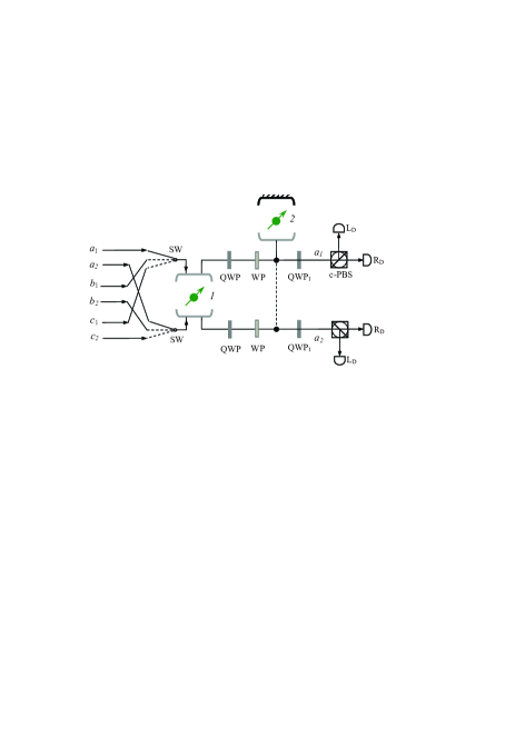
Figure 2: The setup for determining the phase information in polarization and spatial-mode DOFs. QWP represents a quarter-wave plate that can be used to accomplish Hadamard operations on the $|R\rangle$ and $|L\rangle$ polarized states: $|R\rangle\rightarrow\frac{1}{\sqrt{2}}(|R\rangle+|L\rangle)$ and $|L\rangle\rightarrow\frac{1}{\sqrt{2}}(|R\rangle-|L\rangle)$. QWP₁ represents the quarter-wave plate which is different from QWP and can be used to accomplish another Hadamard operation: $|R\rangle\rightarrow\frac{1}{\sqrt{2}}(|R\rangle-|L\rangle)$ and $|L\rangle\rightarrow\frac{1}{\sqrt{2}}(|R\rangle+|L\rangle)$. WP is used to accomplish the single photon operation $\sigma^{i}$ on polarized states: $\sigma^{i}|R\rangle\rightarrow|R\rangle$ and $\sigma^{i}|L\rangle\rightarrow i|L\rangle$. c-PBS is a polarizing beam splitter in the circular basis which transmits the input right-circularly polarized photon $|R\rangle$ and reflects the left-circularly polarized photon $|L\rangle$.

According to the evolution rules of the photon and the spin in the cavity described in Eq. (7), after three photons $ABC$ passes through cavity 1 and the QWPs, the whole system of the three photons and spin 1 evolves as

$$|\Psi^{\pm}_{i}\rangle_{P}|\Phi^{\pm}_{j}\rangle_{S}|+\rangle^{s}_{1} \rightarrow |\Psi^{\mp}_{j}\rangle_{P}|\Phi^{\mp}_{i}\rangle_{S}|-\rangle^{s}_{1},$$

$$|\Psi^{\mp}_{i}\rangle_{P}|\Phi^{\pm}_{j}\rangle_{S}|+\rangle^{s}_{1} \rightarrow |\Psi^{\mp}_{j}\rangle_{P}|\Phi^{\pm}_{i}\rangle_{S}|+\rangle^{s}_{1},$$ (8)

where $|\pm\rangle=\frac{1}{\sqrt{2}}(|\uparrow\rangle\pm|\downarrow\rangle)$, and the overall phase of the system is ignored.

Equation (14) shows that when three photons pass through a double-sided cavity, the states in the polarization DOF and the states in the spatial-mode DOF of the photons $A$, $B$, and $C$ will be interchanged and the phase information in these different DOFs will be flipped. That is, the double-sided cavity works as a SWAP-like gate for these two DOFs. At the same time, the relation between the phase information in these two DOFs will be stored in spin 1. If the phase information in the two DOFs are the same (i.e., the hyperentangled state is in $|\Psi^{\pm}_{i}\rangle_{P}|\Phi^{\pm}_{j}\rangle_{S},i,j=1,2,3$, and $4$), the state of the spin 1 changes to $|-\rangle$ when the photons ABC pass through the double-sided cavity. Otherwise, the spin 1 remains in the state $|+\rangle$ when the phase information in the two DOFs differs (the hyperentangled state is in $|\Psi^{\pm}_{i}\rangle_{P}|\Phi^{\mp}_{j}\rangle_{S}$). Therefore, the spin states divide the states of the $ABC$ photons into two groups: $\{|\Psi^{\pm}_{ABC}\rangle_{P}|\Phi^{\pm}_{ABC}\rangle_{S},|\Psi^{\pm}_{ABC}\rangle_{P}|\Phi^{\mp}_{ABC}\rangle_{S}\}$. Note that, the states in the two different DOFs are interchanged and the phase information in these two DOFs is flipped after the interaction between the photons and spin 1 in the first double-sided cavity.

II.2 Determination of the phase information in polarization DOF based on quantum-dot spin and optical single-sided microcavity system

The second cavity which also involves a singly charged QD embedded in is a single-sided microcavity with the top mirror partially reflective and the bottom mirror 100$\%$ reflective, as shown in Fig.2. The spin of the QD (spin 2) is also prepared in the state $|\Psi_{2}\rangle=(|\uparrow\rangle+|\downarrow\rangle)_{1}/\sqrt{2}$. The different reflection coefficients for the coupling ($r_{h}^{\prime}$) and uncoupling spin-cavity systems ($r_{0}^{\prime}$) can be determined by solving another Heisenberg equations of motion 6 ; 7 ; 13 , and

$$r_{h}^{\prime}(\omega) = 1-\frac{\kappa[i(\omega_{X^{-}}-\omega)+\frac{\gamma}{2}]}{[i(\omega_{X^{-}}-\omega)+\frac{\gamma}{2}][i(\omega_{c}-\omega)+\frac{\kappa}{2}+\frac{\kappa_{s}}{2}]+g^{2}},$$

$$r_{0}^{\prime}(\omega) = \frac{i(\omega_{0}-\omega)+\frac{\kappa_{s}}{2}}{i(\omega_{c}-\omega)+\frac{\kappa}{2}+\frac{\kappa_{s}}{2}}.$$ (9)

By suitable detuning of the photon frequency, the phase difference between $r_{h}^{\prime}$ and $r_{0}^{\prime}$ can be adjusted to $\pi/2$, and a photon-spin phase-shift gate can be developed7 as follows:

$$|R,\uparrow\rangle\rightarrow|L,\uparrow\rangle,\;\;|L,\uparrow\rangle\rightarrow i|R,\uparrow\rangle,$$

$$|R,\uparrow\rangle\rightarrow i|L,\uparrow\rangle,\;\;|L,\uparrow\rangle\rightarrow|R,\uparrow\rangle.$$ (10)

From the Eq. (10), one can see that in the coupling case, the photon will be reflected by the cavity and the state of the photon will be flipped for the unchanged photon spin $s_{z}$. In the uncoupling case, the photon will not only be flipped but also pick up a $\pi/2$ phase when it is reflected by the cavity. This type of spin-cavity unit can be used to determine the phase information in the polarization DOF without destroying the photons $ABC$renoehbsa ; 13 .

As shown in Fig. 2, after passing through the QWPs, which act as the Hadamard operations on the polarization DOF, that is,

$$|R\rangle\rightarrow(|R\rangle+|L\rangle)/\sqrt{2},\;\;\;\;|L\rangle\rightarrow(|R\rangle-|L\rangle)/\sqrt{2},$$ (11)

the eight GHZ states $|\Psi^{\pm}_{j}\rangle_{P}$ ($j=1,2,3,4$) in the polarization DOF evolve as

$$|\Psi^{+}_{1}\rangle_{P} \rightarrow \frac{1}{2}(|RRR\rangle+|RLL\rangle+|LRL\rangle+|LLR\rangle)_{ABC}=|\psi^{+}_{1}\rangle_{P},$$

$$|\Psi^{-}_{1}\rangle_{P} \rightarrow \frac{1}{2}(|LLL\rangle+|LRR\rangle+|RLR\rangle+|RRL\rangle)_{ABC}=|\psi^{-}_{1}\rangle_{P},$$

$$|\Psi^{+}_{2}\rangle_{P} \rightarrow \frac{1}{2}(|RRR\rangle+|RLL\rangle-|LRL\rangle-|LLR\rangle)_{ABC}=|\psi^{+}_{2}\rangle_{P},$$

$$|\Psi^{-}_{2}\rangle_{P} \rightarrow -\frac{1}{2}(|LLL\rangle+|LRR\rangle-|RLR\rangle-|RRL\rangle)_{ABC}=|\psi^{-}_{2}\rangle_{P},$$

$$|\Psi^{+}_{3}\rangle_{P} \rightarrow \frac{1}{2}(|RRR\rangle-|RLL\rangle+|LRL\rangle-|LLR\rangle)_{ABC}=|\psi^{+}_{3}\rangle_{P},$$

$$|\Psi^{-}_{3}\rangle_{P} \rightarrow -\frac{1}{2}(|LLL\rangle-|LRR\rangle+|RLR\rangle-|RRL\rangle)_{ABC}=|\psi^{-}_{3}\rangle_{P},$$

$$|\Psi^{+}_{4}\rangle_{P} \rightarrow \frac{1}{2}(|RRR\rangle-|RLL\rangle-|LRL\rangle+|LLR\rangle)_{ABC}=|\psi^{+}_{4}\rangle_{P},$$

$$|\Psi^{-}_{4}\rangle_{P} \rightarrow \frac{1}{2}(|LLL\rangle-|LRR\rangle-|RLR\rangle+|RRL\rangle)_{ABC}=|\psi^{-}_{4}\rangle_{P}.$$ (12)

From Eq. (12), we can see that, after the Hadamard transformation, the number of $|R\rangle$ is odd for the states $|\Psi^{+}_{j}\rangle_{P}$ with the superscript $+$ while the number of $|R\rangle$ is even for other states, i.e., $|\Psi^{-}_{j}\rangle_{P}$. The eight GHZ states $|\Psi^{\pm}_{j}\rangle_{P}$ can be divided into two groups: $\{|\Psi^{+}_{ABC}\rangle_{P},|\Psi^{-}_{ABC}\rangle_{P}$. With grouping and the single-sided cavity-QD unit which is same as that by Ren et al.renoehbsa , we can complete the task of phase-determination in the polarization DOF. From Fig. 2, when three photons are reflected by cavity 2 and gain a $\frac{\pi}{2}$ phase on all of the $|L\rangle$ photons using wave planes (WPs), the total states of the three photons with one spin are transformed into

$$|\psi^{+}_{1}\rangle_{P}|+\rangle^{s}_{2} \rightarrow \frac{-i}{2}(|LLL\rangle+|LRR\rangle+|RLR\rangle+|RRL\rangle)_{ABC}|+^{\prime}\rangle^{s}_{2},$$

$$|\psi^{-}_{1}\rangle_{P}|+\rangle^{s}_{2} \rightarrow \frac{-i}{2}(|RRR\rangle+|RLL\rangle+|LRL\rangle+|LLR\rangle)_{ABC}|-^{\prime}\rangle^{s}_{2},$$

$$|\psi^{+}_{2}\rangle_{P}|+\rangle^{s}_{2} \rightarrow \frac{-i}{2}(|LLL\rangle+|LRR\rangle-|RLR\rangle-|RRL\rangle)_{ABC}|+^{\prime}\rangle^{s}_{2},$$

$$|\psi^{-}_{2}\rangle_{P}|+\rangle^{s}_{2} \rightarrow \frac{i}{2}(|RRR\rangle+|RLL\rangle-|LRL\rangle-|LLR\rangle)_{ABC}|-^{\prime}\rangle^{s}_{2},$$

$$|\psi^{+}_{3}\rangle_{P}|+\rangle^{s}_{2} \rightarrow \frac{-i}{2}(|LLL\rangle-|LRR\rangle+|RLR\rangle-|RRL\rangle)_{ABC}|+^{\prime}\rangle^{s}_{2},$$

$$|\psi^{-}_{3}\rangle_{P}|+\rangle^{s}_{2} \rightarrow \frac{i}{2}(|RRR\rangle-|RLL\rangle+|LRL\rangle-|LLR\rangle)_{ABC}|-^{\prime}\rangle^{s}_{2},$$

$$|\psi^{+}_{4}\rangle_{P}|+\rangle^{s}_{2} \rightarrow \frac{-i}{2}(|LLL\rangle-|LRR\rangle-|RLR\rangle+|RRL\rangle)_{ABC}|+^{\prime}\rangle^{s}_{2},$$

$$|\psi^{-}_{4}\rangle_{P}|+\rangle^{s}_{2} \rightarrow \frac{-i}{2}(|RRR\rangle-|RLL\rangle-|LRL\rangle+|LLR\rangle)_{ABC}|-^{\prime}\rangle^{s}_{2}.$$ (13)

Here, $|+^{\prime}\rangle^{s}_{2}=\frac{1}{\sqrt{2}}(|\uparrow\rangle+i|\downarrow\rangle)$ and $|-^{\prime}\rangle^{s}_{2}=\frac{1}{\sqrt{2}}(|\uparrow\rangle-i|\downarrow\rangle)$. With an measurement on the spin 2 in basis $\{|+^{\prime}\rangle,|-^{\prime}\rangle\}$, one can read out the information about the phases in the polarization DOF. If the spin 2 is in the state $|+^{\prime}\rangle^{s}_{2}$, the phase information is $+$ in polarization DOF; otherwise, the phase information is $-$, when the measuring result of the spin 2 is $|-^{\prime}\rangle^{s}_{2}$. The relation between the measurement outcomes of spins $1$ and $2$ and the initial phase information of the hyperentangled photons system is shown in Table 1.

From Table 1, one can see that the phase information in two DOFs can be obtained by measuring spins 1 and 2. Electron spin $1$ is measured using the spin basis $\{|+\rangle,|-\rangle\}$ whereas electron spin $2$ is measured using the spin basis $\{|+^{\prime}\rangle,|-^{\prime}\rangle\}$. Spin $1$ records the relation between the phase information in the polarization and spatial-mode DOFs, while spin 2 can be used to determine the initial information encoded in the spatial-mode DOF. In detail, when spin 2 is detected in the state $|+^{\prime}\rangle$, the initial phase information of the photons in the spatial-mode DOF is $-$. When the spin 2 is detected in the state $|-^{\prime}\rangle$, the photons are initially in the spatial-mode state $|\Phi^{+}\rangle_{S}$. The phase information in the polarization DOF can be obtained when the phase information in the spatial-mode DOF is determined and spin 1 is measured using $\{|+\rangle,|-\rangle\}$ as the basis. If spin 1 is in the state $|-\rangle$, the phase information in two DOFs is same; otherwise, the phase information in two DOFs is different when the spin 1 is in the state $|+\rangle$.

Table 1: Relationship between the measurement outcomes of two spins and the initial phase information of the hyperentangled states

	Spin $1$ and $2$		the initial phase information
	$|+\rangle_{1}|+^{\prime}\rangle_{2}$		$|\Psi^{-}\rangle_{P}\otimes|\Phi^{+}\rangle_{S}$
	$|+\rangle_{1}|-^{\prime}\rangle_{2}$		$|\Psi^{+}\rangle_{P}\otimes|\Phi^{-}\rangle_{S}$
	$|-\rangle_{1}|+^{\prime}\rangle_{2}$		$|\Psi^{-}\rangle_{P}\otimes|\Phi^{-}\rangle_{S}$
	$|-\rangle_{1}|-^{\prime}\rangle_{2}$		$|\Psi^{+}\rangle_{P}\otimes|\Phi^{+}\rangle_{S}$

Then, by applying Hadamard transformations on the three photons in the polarization DOF, the the polarization states of the photons $ABC$ are changed back into the standard GHZ-state form. Finally, the photons $ABC$ can be independently measured in both the polarization and spatial-mode DOFs with single-photon detectors. Thus, as shown in Table 2 and 3, the outcomes of three photon polarization states determine the parity information in the spatial-mode DOF, whereas the outcomes of the spatial-mode states determine the parity information in the polarization DOF. The relationship between the measurement outcomes of the states of the three photons $ABC$ and the initial parity information of hyperentangled photon system is shown in Table 2 and 3.

Table 2: Relationship between the final polarization states of three photons and the initial hyperentangled states.

	the final Spatial-mode state		the initial Polarization state
	$|RRR\rangle_{ABC}$, $|LLL\rangle_{ABC}$		$|\Phi^{\pm}_{1}\rangle_{P}$
	$|RRL\rangle_{ABC}$, $|LLR\rangle_{ABC}$		$|\Phi^{\pm}_{2}\rangle_{P}$
	$|RLR\rangle_{ABC}$, $|LRL\rangle_{ABC}$		$|\Phi^{\pm}_{3}\rangle_{P}$
	$|LRR\rangle_{ABC}$, $|RLL\rangle_{ABC}$		$|\Phi^{\pm}_{4}\rangle_{P}$

Table 3: Relationship between the final Spatial-mode states of three photons and the initial hyperentangled states.

	the final Spatial-mode state		the initial Polarization state
	$|a_{1}a_{1}a_{1}\rangle_{ABC}$, $|a_{2}a_{2}a_{2}\rangle_{ABC}$		$|\Psi^{\pm}_{1}\rangle_{P}$
	$|a_{1}a_{1}a_{2}\rangle_{ABC}$, $|a_{2}a_{2}a_{1}\rangle_{ABC}$		$|\Psi^{\pm}_{2}\rangle_{P}$
	$|a_{1}a_{2}a_{1}\rangle_{ABC}$, $|a_{2}a_{1}a_{2}\rangle_{ABC}$		$|\Psi^{\pm}_{3}\rangle_{P}$
	$|a_{2}a_{1}a_{1}\rangle_{ABC}$, $|a_{1}a_{2}a_{2}\rangle_{ABC}$		$|\Psi^{\pm}_{4}\rangle_{P}$

According to the measurement of the final states of photons $ABC$ in the polarization and spatial-mode DOFs and the detection result of the spins $1$ and $2$, the initial hyperentangled-GHZ state of the three photons $ABC$ can be determined. From the analysis above, one can see that three-photon 64 GHZ states can be completely distinguished with the help of QD-cavity systems. Moreover, this device can be generalized to N-photon hyperentangled GHZ states analysis and it can also be used to analysis hyperentangled Bell-state photon-pairs. Compared with the previous worksrenoehbsa , our scheme is much simpler as only two spin-cavity units are used here, not four or more. The two QD spins accomplish the task of phase measurement. With the help of the linear wave plates (QWPs and WPs) and two different spin-cavity units, the phase information in two different DOFs can be obtained without destroying three photons. It shows that our device in Fig. 2 can theoretically accomplish a complete and deterministic HGSA with 100$\%$ success probability.

III Application of the HGSA device in quantum communication

In the previous section, we used two different spin-cavity units to construct a device completing a HGSA. Now, we introduce the application of this device in high-capacity, long-distance quantum communication.

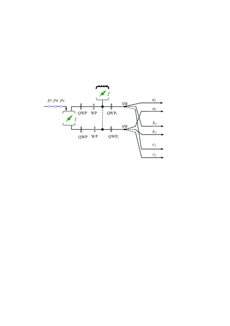
Figure 3: Schematic diagram of hyperentanglement GHZ state generation.

One application of this HGSA device is the generation of hyperentangled-GHZ-state photons. The principle of the hyperentangled GHZ state photon generation (HGSG) is shown in Fig. 3. Three photons, $A$, $B$, and $C$, are prepared in the same initial state $|\varphi_{A}\rangle=|\varphi_{B}\rangle=|\varphi_{C}\rangle=|R\rangle$, and two spins ($1$ and $2$) are prepared in the state $|+\rangle_{1}=|+\rangle_{2}=\frac{1}{\sqrt{2}}(|\uparrow\rangle+|\downarrow\rangle)$. Spin 1 is embedded in a double-sided optical microcavity 1, and spin 2 is embedded in a single-sided optical microcavity 2. Fig. 3 shows that photons $A$, $B$ and $C$ are successively sent into the cavities from the left input port of the HBSG device. After passing through two cavities, the photons can become entangled with the electron-spins. The evolution of the entire system can then be described as

$$|\varphi_{p_{A}}\rangle|\varphi_{p_{B}}\rangle|\varphi_{p_{C}}\rangle|+\rangle_{1}|+\rangle_{2}$$ (14)

$${}^{\underrightarrow{cavity1}} \frac{1}{2}|+\rangle_{2}[|-\rangle_{1}(|\Psi^{-}_{1}\rangle_{P}|\Phi^{-}_{1}\rangle_{S}-|\Psi^{+}_{1}\rangle_{P}|\Phi^{+}_{1}\rangle_{S})_{ABC}$$

$$+\;\;|+\rangle_{1}(|\Psi^{+}_{1}\rangle_{P}|\Phi^{-}_{1}\rangle_{S}-|\Psi^{-}_{1}\rangle_{P}|\Phi^{+}_{1}\rangle_{S})_{ABC}]$$

$${}^{\underrightarrow{QWP}} \frac{1}{2}|+\rangle_{2}[|-\rangle_{1}(|\psi^{-}_{1}\rangle_{P}|\Phi^{-}_{1}\rangle_{S}-|\psi^{+}_{1}\rangle_{P}|\Phi^{+}_{1}\rangle_{S})_{ABC}$$

$$+\;\;|+\rangle_{1}(|\psi^{+}_{1}\rangle_{P}|\Phi^{-}_{1}\rangle_{S}-|\psi^{-}_{1}\rangle_{P}|\Phi^{+}_{1}\rangle_{S})_{ABC}]$$

$${}^{\underrightarrow{WP,\;cavity2}} \frac{-i}{2}(|-\rangle_{1}|-^{\prime}\rangle_{2}|\psi^{+}_{1}\rangle_{ABC_{P}}|\Phi^{-}_{1}\rangle_{ABC_{S}}-|-\rangle_{1}|+^{\prime}\rangle_{2}|\psi^{-}_{1}\rangle_{ABC_{P}}|\Phi^{+}_{1}\rangle_{ABC_{S}}$$

$$+\;\;|+\rangle_{1}|+^{\prime}\rangle_{2}||\psi^{-}_{1}\rangle_{ABC_{P}}|\Phi^{-}_{1}\rangle_{ABC_{S}}-|+\rangle_{1}|-^{\prime}\rangle_{2}||\psi^{+}_{1}\rangle_{ABC_{P}}|\Phi^{+}_{1}\rangle_{ABC_{S}})$$

$${}^{\underrightarrow{QWP_{1}}} \frac{-i}{2}(|-\rangle_{1}|-^{\prime}\rangle_{2}|\Psi^{-}_{1}\rangle_{ABC_{P}}|\Phi^{-}_{1}\rangle_{ABC_{S}}-|-\rangle_{1}|+^{\prime}\rangle_{2}|\Psi^{+}_{1}\rangle_{ABC_{P}}|\Phi^{+}_{1}\rangle_{ABC_{S}}$$

$$+\;\;|+\rangle_{1}|+^{\prime}\rangle_{2}||\Psi^{+}_{1}\rangle_{ABC_{P}}|\Phi^{-}_{1}\rangle_{ABC_{S}}-|+\rangle_{1}|-^{\prime}\rangle_{2}||\Psi^{-}_{1}\rangle_{ABC_{P}}|\Phi^{+}_{1}\rangle_{ABC_{S}}),$$

Eq. (14) shows that the spins $1$ and $2$ in the cavities record the phase information in these two DOFs. If spin 2 is in the state $|+^{\prime}\rangle$, the phase information in spatial-mode DOF is ‘+’; otherwise the phase information in the spatial-mode DOF is ‘-’ when spin 2 is in the state $|-^{\prime}\rangle$. If the final state of the photon is $|\Psi^{\pm}_{1}\rangle_{P}|\Phi^{\pm}_{1}\rangle_{S}$, i.e., the phase information in two DOFs is the same, the spin 1 changes into the state $|-\rangle$ when the photons $ABC$ pass through the cavity 1. Otherwise, the state of the spin 1 remains unchanged in $|+\rangle$ when the phase information in the two DOFs differs (the hyperentangled state is either one of $|\Psi^{+}_{1}\rangle_{P}|\Phi^{-}_{1}\rangle_{S}$ and $|\Psi^{-}_{1}\rangle_{P}|\Phi^{+}_{1}\rangle_{S}$). The relationship between the measurement outcomes of the two spins and the hyperentangled states of the photon system is shown in Table 4. By measuring two-electron spins $1$ and $2$ using the spin basis $\{|+\rangle,|-\rangle\}$ 7 ; 9 , one can determine the hyperentangled states of the two photons. By far, we have described the scheme of our HGSG using the QD-cavity systems.

Table 4: The relation between the outcomes of the states of the two spins and the obtained final hyperentangled state.

	Spin $1$ and $2$		Hyperentangled state
	$|-\rangle_{1}|-^{\prime}\rangle_{2}$		$|\Psi^{-}_{1}\rangle_{P}\otimes|\Phi^{-}_{1}\rangle_{S}$
	$|-\rangle_{1}|+^{\prime}\rangle_{2}$		$|\Psi^{+}_{1}\rangle_{P}\otimes|\Phi^{+}_{1}\rangle_{S}$
	$|+\rangle_{1}|+^{\prime}\rangle_{2}$		$|\Psi^{+}_{1}\rangle_{P}\otimes|\Phi^{-}_{1}\rangle_{S}$
	$|+\rangle_{1}|-^{\prime}\rangle_{2}$		$|\Psi^{-}_{1}\rangle_{P}\otimes|\Phi^{+}_{1}\rangle_{S}$

As the HBSG source and the complete and deterministic HGSA are important to quantum communication, it is necessary to discuss the applications of HGSG and HGSA. Here, we use hyperentanglement swapping with the present spin-cavity device as an example and describe its application in manipulating multiparticle entanglement (see Fig. 5). An interesting situation arises when hyperentanglement swapping is exploited to manipulate multiparticle hyperentanglement. Hyperentanglement swapping enables multi-parties that are far from each other in quantum communication to simultaneously share one hyperentangled-state without directly interacting with each other. First, we assume that three hyperentangled three-photon GHZ states $|\varphi\rangle_{145}$, $|\varphi\rangle_{267}$ and $|\varphi\rangle_{389}$ are prepared in the same state$|\Psi^{+}_{1}\rangle_{P}|\Phi^{+}_{1}\rangle_{S}$ and shared by a central exchanger (Ex) and six users $A,B,C,D,E,F$, and $F$ at different locations in a quantum network (see Fig. 5). After GHZ hyperentanglement swapping, the whole system which consists of nine photons, becomes

$$\frac{1}{8}\;(|\Psi^{+}_{1}\rangle_{123}|\Psi^{+}_{1}\rangle_{456789}+|\Psi^{-}_{1}\rangle_{123}|\Psi^{-}_{1}\rangle_{456789}+|\Psi^{+}_{2}\rangle_{123}|\Psi^{+}_{2}\rangle_{456789}+|\Psi^{-}_{2}\rangle_{123}|\Psi^{-}_{2}\rangle_{456789}$$

$$\;\;+\;\;|\Psi^{+}_{3}\rangle_{123}|\Psi^{+}_{3}\rangle_{456789}+|\Psi^{-}_{3}\rangle_{123}|\Psi^{-}_{3}\rangle_{456789}+|\Psi^{+}_{4}\rangle_{123}|\Psi^{+}_{4}\rangle_{456789}+|\Psi^{-}_{4}\rangle_{123}|\Psi^{-}_{4}\rangle_{456789})_{P}$$

$$\;\;\otimes\;\;(|\Phi^{+}_{1}\rangle_{123}|\Phi^{+}_{1}\rangle_{456789}+|\Phi^{-}_{1}\rangle_{123}|\Phi^{-}_{1}\rangle_{456789}+|\Phi^{+}_{2}\rangle_{123}|\Phi^{+}_{2}\rangle_{456789}+|\Phi^{-}_{2}\rangle_{123}|\Phi^{-}_{2}\rangle_{456789}$$

$$\;\;+\;\;|\Psi^{+}_{3}\rangle_{123}|\Psi^{+}_{3}\rangle_{456789}+|\Psi^{-}_{3}\rangle_{123}|\Psi^{-}_{3}\rangle_{456789}+|\Phi^{+}_{4}\rangle_{123}|\Phi^{+}_{4}\rangle_{456789}+|\Phi^{-}_{4}\rangle_{123}|\Phi^{-}_{4}\rangle_{456789})_{S},$$ (15)

where

$$|\Psi^{\pm}_{1}\rangle_{456789}=\frac{1}{\sqrt{2}}(|RRRRRR\rangle\pm|LLLLLL\rangle)_{456789},$$

$$|\Psi^{\pm}_{2}\rangle_{456789}=\frac{1}{\sqrt{2}}(|RRRRLL\rangle\pm|LLLLRR\rangle)_{456789},$$

$$|\Psi^{\pm}_{3}\rangle_{456789}=\frac{1}{\sqrt{2}}(|RRLLRR\rangle\pm|LLRRLL\rangle)_{456789},$$

$$|\Psi^{\pm}_{4}\rangle_{456789}=\frac{1}{\sqrt{2}}(|LLRRRR\rangle\pm|RRLLLL\rangle)_{456789},$$ (16)

and

$$|\Phi^{\pm}_{1}\rangle_{456789}=\frac{1}{\sqrt{2}}(|a_{1}b_{1}c_{1}d_{1}e_{1}f_{1}\rangle\pm|a_{2}b_{2}c_{2}d_{2}e_{2}f_{2}\rangle)_{456789},$$

$$|\Phi^{\pm}_{2}\rangle_{456789}=\frac{1}{\sqrt{2}}(|a_{1}b_{1}c_{1}d_{1}e_{2}f_{2}\rangle\pm|a_{2}b_{2}c_{2}d_{2}e_{1}f_{1}\rangle)_{456789},$$

$$|\Phi^{\pm}_{3}\rangle_{456789}=\frac{1}{\sqrt{2}}(|a_{1}b_{1}c_{2}d_{2}e_{1}f_{1}\rangle\pm|a_{2}b_{2}c_{1}d_{1}e_{2}f_{2}\rangle)_{456789},$$

$$|\Phi^{\pm}_{4}\rangle_{456789}=\frac{1}{\sqrt{2}}(|a_{2}b_{2}c_{1}d_{1}e_{1}f_{1}\rangle\pm|a_{1}b_{1}c_{2}d_{2}e_{2}f_{2}\rangle)_{456789},$$ (17)

are eight orthogonal GHZ states in the polarization and the spatial-mode DOFs spanning the whole three-qubit Hilbert space. Here, $x_{1}$ and $x_{2}$ ($x=a,b,c,d,e$, and $f$) are different spatial-modes for the photon holed by user $X$ ($X=A,B,C,D,E,$ and $F$). It is clear from Eq. (15) that the six distant photon belonging to A, B, C, D, E, and F will be subsequently entangled into one of the 64 GHZ hyperentangled states according to Ex s measurement result. Thus, the generation and distribution of multiparticle entangled states is achieved. As an application, this network configuration can work as a quantum telephone exchanger quantele . By using hyperentangled GHZ states, the transmission capacity of the channels can be twice as effective as normal quantum communication schemes which use photon-pairs entangled in only one DOF. The quantum network can be extended to N user by using the same principle. This QD-cavity system can also be realized in other physical systems, such atom-cavity system atomswap and NV-center-cavity system for similarly relevant levels.

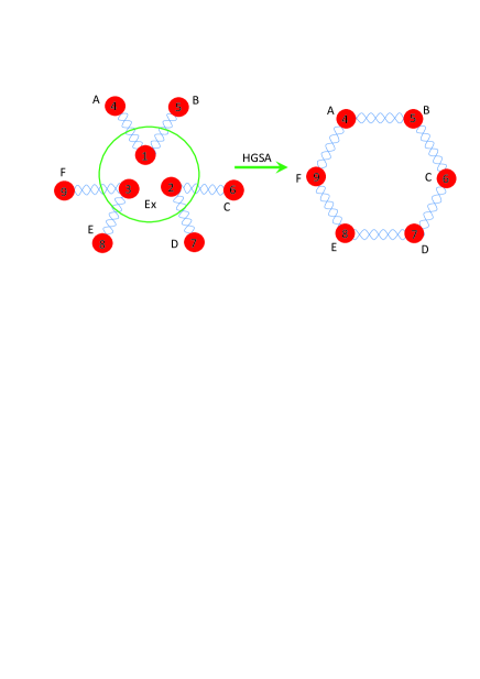
Figure 4: Schematic diagram of GHZ hyperentanglement swapping.

IV DISCUSSION AND CONCLUSION

In this section, we discuss the fidelity of using HBSG and HBSA in a promising system with GaAs-or InAs-based QDs in micropillar microcavities. The core component of our protocol is the spin-cavity units of which the fidelity and efficiency are discussed in Ref. hybrid ; 7 . In the present hyperentangled-state analysis scheme, the first spin-cavity unit acts as a SWAP gate, that directly swaps the initial states in the polarization and spatial-mode DOFs and then records the relation between the phase information in two DOFs.

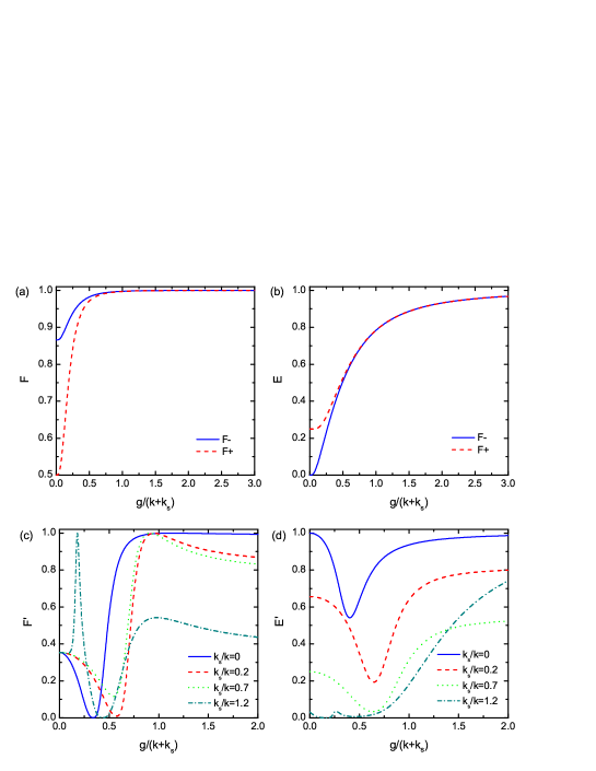
Figure 5: Fidelity (a) and efficiency (b) of the double-sided cavity unit via the coupling strength $g/(\kappa+\kappa_{s})$ when $|t_{0}|=|r_{h}|$. $F_{+}$ and $F_{-}$ represent the fidelity of the present scheme when the outcomes of spin 1 are $|+\rangle$ and $|-\rangle$, respectively. Fidelity (c) and efficiency (d) of the double-sided cavity unit via the coupling strength $g/(\kappa+\kappa_{s})$ and different $\kappa_{s}/\kappa$. $F^{\prime}$ and $E^{\prime}$ represent the fidelity and efficiency of the single-sided cavity, respectively.

To simplify, we consider the case $|t_{0}(\omega)|=|r_{h}(\omega)|$, in which the fidelities to generate (or analyze ) $|\phi^{-}_{AB}\rangle_{P}\otimes|\phi^{+}_{AB}\rangle_{S}$, $|\phi^{+}_{AB}\rangle_{P}\otimes|\psi^{-}_{AB}\rangle_{S}$, $|\psi^{+}_{AB}\rangle_{P}\otimes|\psi^{-}_{AB}\rangle_{S}$, and $|\psi^{-}_{AB}\rangle_{P}\otimes|\phi^{+}_{AB}\rangle_{S}$ can remain in unity, whereas the fidelity to generate (or analyze) 12 other hyperentangled Bell states are generally less than one, depending on the difference between $|t_{0}|$ and $|r_{0}|$. The fidelity (in amplitude) is given by

$$F_{-}=\frac{|r_{0}^{3}+t_{0}^{3}|}{\sqrt{(r_{0}^{3}+t_{0}^{3})^{2}+3(r_{0}^{2}t_{0}+t_{0}^{2}r_{0})^{2}}},\;\;\;\;F_{+}=\frac{|r_{0}^{3}-t_{0}^{3}|}{\sqrt{(r_{0}^{3}-t_{0}^{3})^{2}+3(r_{0}^{2}t_{0}-t_{0}^{2}r_{0})^{2}}},$$ (18)

and the corresponding efficiencies are

$$E_{-}=(r_{0}^{3}+t_{0}^{3})^{2}+3(r_{0}^{2}t_{0}+t_{0}^{2}r_{0})^{2},\;\;\;\;E_{+}=(r_{0}^{3}-t_{0}^{3})^{2}+3(r_{0}^{2}t_{0}-t_{0}^{2}r_{0})^{2}.$$ (19)

Here, $F_{+}$ ($E_{+}$) and $F_{-}$ ($E_{-}$) represent the fidelity (efficiency) of the present scheme when the outcomes of the spin 1 states are $|+\rangle$ and $|-\rangle$, respectively.

For the single-sided cavity, the fidelity $F^{\prime}$ used to measure the phase in the polarization DOF is

$$F^{\prime} = \frac{|r_{h}^{\prime}(r_{h}^{\prime 2}-3r_{0}^{2})+i(r_{0}^{\prime 2}-3r_{h}^{\prime 2})r_{0}^{\prime}|}{2\sqrt{2[|r_{0}^{\prime 3}|^{2}+|r_{h}^{\prime 3}|^{2}+3(|r_{0}^{\prime 2}r_{h}^{\prime}|^{2}+|r_{h}^{\prime 2}r_{0}^{\prime}|^{2})]}},$$ (20)

and the corresponding efficiency $E^{\prime}$ is

$$E^{\prime} = \frac{|r_{0}^{\prime 3}|^{2}+|r_{h}^{\prime 3}|^{2}+3(|r_{0}^{\prime 2}r_{h}^{\prime}|^{2}+|r_{h}^{\prime 2}r_{0}^{\prime}|^{2})}{8}.$$ (21)

Fig. 5 illustrates numerical calculations of the fidelity and efficiency of the device versus the coupling strength $g/(\kappa_{s}+\kappa)$ and different $\kappa_{s}/\kappa$. A low $\kappa_{s}/\kappa$ in the strong coupling regime can induce high fidelity and efficiency in both the double-sided and single-sided cavity systems. In the ideal case, where $g/(\kappa+\kappa_{s})>1.5$ and $\kappa_{s}/\kappa\ll 1$, near-unity fidelity and near-unity efficiency ($F_{+}=F_{-}=F^{\prime}\sim 1$, $E>90\%$, and $E^{\prime}>97\%$ ) can be simultaneously achieved. Given the cavity loss and $g/(\kappa+\kappa_{s})<1.5$, high fidelity still can be achieved but the corresponding efficiency is lower than $0.9$. In the current experiment, a large(7.3 $\mu$m diameter) micropillar cavity can be used to construct the double-sided cavity system. Strong coupling in this cavity has been observed. The quality factor Q can be improved to $\sim 6.5\times 10^{4}$, $\kappa_{s}/\kappa=0.36$ and the corresponding coupling strength is $g/(\kappa_{s}+\kappa)\simeq 0.8$ 24 . As pointed out in Ref. 13 , a lower $\kappa_{s}/\kappa$ can be obtained by thinning down the top mirrors of the high-Q micropillars to achieve effective system parameters: $\kappa_{s}/\kappa\simeq 0.2$ and $Q\sim 4.3\times 10^{4}$. In this case, the system now remains in the strong coupling regime with $g/(\kappa+\kappa_{s})\simeq 0.58$ thindown , the fidelities $F_{+}$ and $F_{-}$ can reach $0.99$ and the corresponding efficiency $E_{+}=E_{-}=60\%$. A single-sided spin unit can be constructed by using small micropillar cavities. Effective system parameters: $\kappa_{s}/\kappa\simeq 0.7$, $g/(\kappa_{s}+\kappa)\simeq 1.0$ can be achieved in strong-coupling regime with diameter around $1.5\mu m$ for the In(Ga)As QD-cavity system13 . A near-unity fidelity can be achievable with $E^{\prime}=20\%$. From Figs.5 (c) and 5 (d), in the small loss limit ($\kappa_{s}/\kappa\approx 0.2$), a near-unity fidelity $F^{\prime}\sim 0.98$ and efficiency $E^{\prime}=52\%$ can be achieved at point $g/(\kappa+\kappa_{s})=0.88$. We thus prove that the present scheme can work in the strong-coupling regimes within current technology.

The fidelities of HGSG operations decreases because of spin decoherence by a factor of $F^{\prime}=[1+exp(-5t/T)]/2$ hybrid , where $T$ is the electron-spin coherence time ($\sim\mu s$ 5 ) and $t$ is the time interval between the different photon spatial-mode states. $5t$ should be considerably shorter than $T$ and $t$ should be longer than $\tau/n_{0}\sim ns$ 9 , where $\tau$ is the cavity photon lifetime and $n_{0}$ is the critical photon number of the spin-cavity system 52 . The single spin can be measured non-destructively by using photon-spin entanglement. After applying a Hadamard gate on the electron spin, the spin superposition states $|+\rangle$ and $|-\rangle$ can be transformed into the spin states $|\uparrow\rangle$ and $|\downarrow\rangle$, respectively, and the spin can be detected in the $|\uparrow\rangle$ and $|\downarrow\rangle$ basis by measuring the helicity of the transmitted or reflected photon. As discussed in Ref. hybrid , the spin superposition state $|+\rangle$ and $|-\rangle$ can be made from the spin eigenstates by using nanosecond ESR pulses or picosecond optical pulses 52 .

In summary, we propose a scheme that can be used to not only completely distinguish the 64 hyperentangled GHZ states in both polarization and spatial-mode DOFs but also to produce three-photon hyperentangled GHZ states using the QD-cavity system. By using numerical calculations, we illustrate that our gate may be feasible for use with the current technologies. In the strong coupling regime, we expect near-unity fidelity and $>52\%$ efficiency in both steps of phase measurement. The proposed HGSA and HGSG device can be applied as a crucial components in high-capacity, long-distance quantum communication. In this work, we demonstrated how to apply this device in hyperentanglement quantum swapping. With the help of hyperentanglement generation and analysis, the spin-cavity units can not only work in constructing large-scale quantum communication networks but also help in other aspects of quantum information science and technology.

References

- (1) R. Raussendorf and H. J. Briegel, “A one-way quantum computer”, Phys. Rev. Lett. 86, 5188 (2001).
- (2) C. H. Bennett, G.Brassard, C. Crépeau, R. Jozsa, A. Peres, and W. K. Wootters, “Teleporting an unknown quantum state via dual classical and Einstein-Podolsky-Rosen channels”, Phys. Rev. Lett. 70, 1895 (1993)
- (3) C. H. Bennett and S. J. Wiesner, “Communication via one-and two-particle operators on Einstein-Podolsky-Rosen states,” Phys. Rev. Lett. 69, 2881 (1992).
- (4) A. K. Ekert, “Quantum cryptography based on Bell’s theorem”, Phys. Rev. Lett. 67, 661 (1991).
- (5) D. M. Greenberger, M. A. Horne, A. Shimony, and A. Zeilinger, “Bell s theorem without inequalities”, Am. J. Phys. 58, 1131 C1143 (1990).
- (6) A. Zeilinger, M. A. Horne, H. Weinfurter, and M. Zukowski, “Three-Particle Entanglements from Two Entangled Pairs”, Phys. Rev. Lett. 78, 3031 (1997); D. Bouwmeester, J.-W. Pan, M. Daniell, H. Weinfurter, and A. Zeilinger, “Observation of Three-Photon Greenberger-Horne-Zeilinger Entanglement ”, Phys. Rev. Lett. 82, 1345 (1999).
- (7) L. Quiroga and N. F. Johnson, “Entangled Bell and Greenberger-Horne-Zeilinger States of Excitons in Coupled Quantum Dots”, Phys. Rev. Lett. 83, 2270(1999)
- (8) Wen-An Li and Lian-Fu Wei, “Controllable entanglement preparations between atoms in spatially-separated cavities via quantum Zeno dynamics”, Opt. Express 20, 13440 (2012).
- (9) Anshou Zheng, Jiahua Li, Rong Yu, Xin-You Lü and Ying Wu, “Generation of Greenberger-Horne-Zeilinger state of distant diamond nitrogen-vacancy centers via nanocavity input-output process”, Opt. Express 20, 16902 (2012).
- (10) A. Karlsson and M. Bourennane, “Quantum teleportation using three-particle entanglement”, Phys. Rev. A 58, 4394 C4400 (1998); E. Jung, M. R. Hwang, H. JuYou, M. S. Kim, S. K. Yoo, H. Kim, D. Park, J. W. Son, S. Tamaryan, and S. K. Cha, “ Greenberger CHorne CZeilinger versusWstates: quantum teleportation through noisy channels”, Phys. Rev. A 78, 012312 (2008).
- (11) C. Y. Lu, T. Yang, and J. W. Pan, “ Experimental multiparticle entanglement swapping for quantum networking”, Phys. Rev. Lett. 103, 020501 (2009).
- (12) Greenberger, D.M., Horne, M.A., Zeilinger, A.: In: Kafatos, M. (ed.)Bell s Theorem, Quantum Theory, and Conceptions of the Universe, Kluwer, Dordrecht (1989); D. M. Greenberger, M. A. Horne, A. Shimony, and A. Zeilinger, “Bells theorem without inequalities”, Am. J. Phys. 58, 1131 C1143 (1990).
- (13) Yan Xia, Qing-Qin Chen, Jie Song, and He-Shan Song, “Efficient hyperentangled Greenberger CHorne CZeilinger states analysis with cross-Kerr nonlinearity”, J. Opt. Soc. Am. B 29, 5 (2012).
- (14) A. Karlsson and M. Bourennane, “Quantum teleportation using three-particle entanglement”, Phys. Rev. A 58, 4394 (1998)
- (15) F. G. Deng, C. Y. Li, Y.S. Li, H. Y. Zhou, and Y. Wang, “Symmetric multiparty-controlled teleportation of an arbitrary two-particle entanglement”, Phys. Rev. A 72, 022338 (2005).
- (16) C. Wang, F. G. Deng, Y. S. Li, X. S. Liu, and G. L. Long, “Quantum secure direct communication with high-dimension quantum superdense coding”. Phys. Rev. A 71, 044305 (2005).
- (17) X. S. Liu, G. L. Long, D. M. Tong, and L. Feng, “General scheme for super dense coding between multi-parties”, Phys. Rev. A 65,022304 (2002).
- (18) J. W. Pan, A. Zeilinger, “Greenberger CHorne CZeilinger-state analyzer”, Phys. Rev. A 57, 2208 (1998).
- (19) S. P. Walborn, S. Pdua”, and C. H. Monken, “Hyperentanglement-assisted Bell-state analysis , Phys. Rev. A 68, 042313 (2003).
- (20) C. Schuck, G. Huber, C. Kurtsiefer, and H. Weinfurter, “Complete deterministic linear optics Bell state analysis”, Phys. Rev. Lett. 96, 190501 (2006).
- (21) M. Barbieri, G. Vallone, P. Mataloni, and F. De Martini, “Complete and deterministic discrimination of polarization Bell states assisted by momentum entanglement”, Phys. Rev. A 75, 042317 (2007).
- (22) S. Y. Song, Y. Cao, Y. B. Sheng and G. L. Long, “Complete Greenberger CHorne CZeilinger state analyzer using hyperentanglement”, Quantum Inf. Process, online: DOI 10.1007/s11128-012-0375-x
- (23) M. M. Wilde, and D. B. Uskov, “Linear-optical hyperentanglement-assisted quantum error-correcting code”, Phys. Rev. A 79, 022305 (2009)
- (24) D. Bruss and C. Macchiavello, “Optimal eavesdropping in cryptography with three-dimensional quantum states”, Phys. Rev. Lett. 88, 127901 (2002); N. J. Cerf, M. Bourennane, A. Karlsson, and N. Gisin, “Security of Quantum Key Distribution Using d-Level Systems”, Phys. Rev. Lett. 88, 127902 (2002).
- (25) T. J. Wang, S. Y. song, and G. L. Long, “Quantum repeater based on spatial entanglement of photons and quantum-dot spins in optical microcavities”, Phys. Rev. A 85, 062311 (2012).
- (26) C. Simon and J. W. Pan, “Polarization Entanglement Purification using Spatial Entanglement”, Phys. Rev. Lett. 89, 257901 (2002).
- (27) Y. B. Sheng, F. G. Deng, and G. L. Long, “Complete hyperentangled-Bell-state analysis for quantum communication”, Phys. Rev. A 82, 032318 (2010).
- (28) J. H. Shapiro, “Single-photon Kerr nonlinearities do not help quantum computation”, Phys. Rev. A 73, 062305 (2006).
- (29) J. Gea-Banacloche, “Impossibility of large phase shifts via the giant Kerr effect with single-photon wave packets”, Phys. Rev. A 81, 043823 (2010).
- (30) T. Calarco, A. Datta, P. Fedichev, E. Pazy, and P. Zoller, “Spin-based all-optical quantum computation with quantum dots: Understanding and suppressing decoherence”, Phys. Rev. A 68, 012310 (2003).
- (31) C. Y. Hu, A. Young, J. L. O’Brien, W. J. Munro, and J. G. Rarity, “Giant optical Faraday rotation induced by a single-electron spin in a quantum dot: Applications to entangling remote spins via a single photon”, Phys. Rev. B 78, 085307 (2008).
- (32) C. Y. Hu, W. J. Munro, and J. G. Rarity, “Deterministic photon entangler using a charged quantum dot inside a microcavity”, Phys. Rev. B 78, 125318 (2008).
- (33) C. Y. Hu, W. J. Munro, J. L. O Brien, and J. G. Rarity, “Proposed entanglement beam splitter using a quantum-dot spin in a double-sided optical microcavity”, Phys. Rev. B 80, 205326 (2009).
- (34) C. Bonato, F. Haupt, S. S. R. Oemrawsingh, J. Gudat, D. P. Ding, M. P. van Exter, and D. Bouwmeester, “CNOT and Bell-state analysis in the weak-coupling cavity QED regime”, Phys. Rev. Lett. 104, 160503 (2010).
- (35) C. Y. Hu and J. G. Rarity, “Loss-resistant state teleportation and entanglement swapping using a quantum-dot spin in an optical microcavity”, Phys. Rev. B 83, 115303 (2011).
- (36) B. C. Ren, H. R. Wei, M. Hua, T. Li, F. G. Deng, “Complete hyperentangled-Bell-state analysis for photon systems assisted by quantum-dot spins in optical microcavities”, Opt. Express 20, 24664 (2012).
- (37) Tie-Jun Wang, Yao Lu, and Gui Lu Long, Generation and complete analysis of the hyperentangled-Bell-state for photons assisted by quantum-dot spins in optical microcavities”, Phys. Rev. A 86, 042337 (2012).
- (38) A. Aufféves-Garnier, C. Simon, J. M. Gérard, and J. P. Poizat, “Giant optical nonlinearity induced by a single two-level system interacting with a cavity in the Purcell regime”, Phys. Rev. A 75, 053823 (2007).
- (39) A. M. Stephens, Z. W. E. Evans, S. J. Devitt, A. D. Greentree, A. G. Fowler, W. J. Munro, J. L. O Brien, K. Nemoto, and L. C. L. Hollenberg, “Deterministic optical quantum computer using photonic modules”, Phys. Rev. A 78, 032318 (2008).
- (40) C. Wang, Y. Zhang, and G. S. Jin, “Entanglement purification and concentration of electron-spin entangled states using quantum-dot spins in optical microcavities”, Phys. Rev. A 84, 032307 (2011).
- (41) C. Wang, Y. Zhang, and R. Zhang, “Entanglement purification based on hybrid entangled state using quantum-dot and microcavity coupled system”, Opt. Express 19, 25685 (2011).
- (42) S. Bose, V. Vedral, and P. L. Knight, “Multiparticle generalization of entanglement swapping”, Phys. Rev. A 57, 822 (1998).
- (43) K. Koshino, S. Ishizaka, and Y. Nakamura, “Deterministic photon-photon gate using a system”, Phys. Rev. A 82, 010301(R) (2010).
- (44) V. Loo, L. Lanco, A. Lemaitre, I. Sagnes, O. Krebs, P. Voisin, and P. Senellart, “Quantum dot-cavity strong-coupling regime measured through coherent reflection spectroscopy in a very high-Q micropillar”, Appl. Phys. Lett. 97, 241110 (2010).
- (45) Here g and can be controlled independently as g is determined by the trion oscillator strength and the cavity modal volume, whereas by the cavity quality factor only 13 .
- (46) J. M. Elzerman, R. Hanson, L. H. W. van Beveren, B. Witkamp, L. M. K. Vandersypen, and L. P. Kouwenhoven, “Single-shot read-out of an individual electron spin in a quantum dot”, Nature (London) 430, 431 (2004); M. Kroutvar, Y. Ducommun, D. Heiss, M. Bichler, D. Schuh, G. Abstreiter, and J. J. Finley, “Optically programmable electron spin memory using semiconductor quantum dots”, Nature (London) 432, 81 (2004).
- (47) H. J. Kimble, in Cavity Quantum Electrodynamics, edited by P. Berman (Academic Press, San Diego, 1994).