A one-dimensional spin-orbit interferometer

Abstract

We demonstrate that the combination of an external magnetic field and the intrinsic spin-orbit interaction results in nonadiabatic precession of the electron spin after transmission through a quantum point contact (QPC). We suggest that this precession may be observed in a device consisting of two QPCs placed in series. The pattern of resonant peaks in the transmission is strongly influenced by the non-abelian phase resulting from this precession. Moreover, a novel type of resonance which is associated with suppressed, rather than enhanced, transmission emerges in the strongly nonadiabatic regime. The shift in the resonant transmission peaks is dependent on the spin-orbit interaction and therefore offers a novel way to directly measure these interactions in a ballistic 1D system.

I Introduction

In recent years, it has been recognized that the existence of interactions which couple spin to orbital motion gives rise to the possibility of manipulating the spin via external gates, leading to the suggestion of spintronic devices which require only electric fields for their operation DattaDas . The importance of the spin-orbit interactions lies both in their role in spin dephasing via the Dyakonov-Perel SR:DyakonovPerel1 ; SR:DyakonovPerel2 and Elliot-Yafet SR:Elliott ; SR:Yafet mechanisms, as well as in the potential creation of spin-polarized current SF:Eto ; SF:Gelabert ; SF:GovernaleZulicke2003 ; SF:GovernaleZulicke2004 ; SF:Kita2004 ; SF:LiuZhou ; SF:Xiao .

In the present work we investigate the possibility of the dynamical manipulation of spin via a combination of electric and magnetic fields in a one-dimensional system. We consider the interactions which couple to the first power of spin and therefore have the structure of a magnetic dipole. In the literature, the dominant interaction of this form is usually considered to be due to the inversion asymmetry of the two-dimensional (2D) interface, known as the Rashba effect, while the Dresselhaus effect arising from inversion asymmetry in the bulk crystal has been considered to be negligibly small. While for the narrow-gap semiconductors InAs and InSb, the Rashba interaction is dominant, the coefficient of the Rashba interaction varies by two orders of magnitude between the narrow-gap and medium-gap materials WinklerBook and we expect that in GaAs the situation is reversed. It has previously been possible to determine the relative size of the Rashba and Dresselhaus interactions in 2D GaAs via Faraday rotation MeierSalis , where they were determined to be approximately equal in magnitude. The Dresselhaus interaction was also found to be approximately constant over a range of samples, which is puzzling since it is expected to scale quadratically with the width of the quantum well, as was noted by the authors of MeierSalis .

The dipolar structure of the Rashba and Dresselhaus interactions determines effective magnetic fields which, in the presence of an external magnetic field, will align spin along the direction given by their vector sum with the external field. As existing measurements of the spin-orbit interaction in 2D systems rely on diffusive transport when both the Rashba and Dresselhaus interactions are proportional to the very small average momentum resulting in a small effective magnetic field of order of 1mT. In contrast, in a ballistic system, the spin-orbit interactions are proportional to the Fermi momentum $k_{F}$, which is several orders of magnitude higher than the average momentum in the diffusive regime. We therefore suggest a novel method to measure the spin-orbit interactions in a quantum wire which relies on spin-orbit induced nonadiabaticity inside a ballistic channel.

For simplicity, we consider a quantum point contact formed from a 2D electron gas with only the Dresselhaus interaction present, although we also found numerically that hole systems show similar behaviour. For a wire oriented along the $x=(100)$ direction, we find upon projection of the bulk Hamiltonian onto one-dimensional (1D) states,

$$H_{D}=b^{6c6c}_{41}(p_{x}(p_{y}^{2}-p_{z}^{2})\sigma_{x}+p_{y}(p_{z}^{2}-p_{x}^{2})\sigma_{y}+$$ (1)

$$p_{z}(p_{x}^{2}-p_{y}^{2})\sigma_{z})\rightarrow b^{6c6c}_{41}p_{x}(p_{y}^{2}-p_{z}^{2})\sigma_{x}\ ,$$

where $b^{6c6c}_{41}\approx 28\text{eV}\AA^{3}\hbar^{-3}$ is the Dresselhaus constant WinklerBook , and we have set $\langle p_{y}\rangle=\langle p_{z}\rangle=0$, assuming that the $y$- and $z$ confinements are along (010) and (001) respectively. Here $\sigma_{i}$ are the Pauli matrices describing spin.

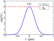
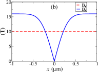
According to Eq. (1) the Dresselhaus magnetic field is parallel to the wire. The field is inhomogeneous in the presence of an electrostatic barrier, Fig.1a, since the effective magnetic field is proportional to the momentum which vanishes semiclassically at the turning points. When an external magnetic field is applied perpendicular to the contact, the combination of the Zeeman interaction and the Dresselhaus interaction forms a total driving torque on spin which is inhomogeneous in space and rapidly switches direction, see Fig.1b. We propose that the non-trivial spin dynamics resulting from the inhomogeneous driving field may be observed in a double barrier interference experiment, and such an experiment will distinguish between adiabatic and nonadiabatic spin motion and therefore serve as a direct measurement of the size of the Dresselhaus interaction. The same logic is applicable to the Rashba interaction.

Figure 1: (Color online). (a) The solid blue line shows the effective potential in a single QPC, modelled as a gaussian, the length of the channel is 2$\mu$m. The dashed red line shows the Fermi energy. (b) The components of the effective magnetic field parallel (blue, solid) and perpendicular (red, dashed) to the QPC. The perpendicular component is the external magnetic field. The parallel component is the Dresselhaus effective field, which decreases semiclassically at the top of the potential shown in the panel (a).

The structure of the paper is as follows: In Section II we formulate the concept of nonadiabatic spin precession and present the criteria for its existence, based on typical experimental parameters. In Section III we introduce the idea of an interferometer consisting of a double quantum point contact (DQPC), and the discuss the adiabaticity of the “orbital” dynamics which is required for interference to be observed. In Section IV we present results of numerical solution of the Schrodinger equation describing electron transmission through the interferometer in the presence of external magnetic and spin-orbit fields, and demonstrate how measurement of the Dresselhaus/Rashba interaction can be performed in the device. In Section V we present the physical mechanism behind the phenomenon of “negative” resonances which are observed in the numerical result and show that they are a strong signature of nonadiabatic spin dynamics. In Section VI we present our conclusions.

II nonadiabaticity due to spin

We consider a one-dimensional channel formed by electrostatic confinement in a 2D electron gas (2DEG) in GaAs, where the 2D quantum well is grown along the (100) direction. In the presence of an external magnetic field and the Dresselhaus interaction the conductance is determined by the solution of the spin-dependent transmission problem. The effective Hamiltonian for a single channel reads

$$H=\frac{p_{x}^{2}}{2m}+U(x)-\frac{1}{2}g^{*}\mu_{B}\vec{B}\cdot\vec{\sigma}+b^{6c6c}_{41}p_{x}(p_{y}^{2}-p_{z}^{2})\sigma_{x}\ ,$$ (2)

where $U(x)$ is the electrostatic barrier, for GaAs, $m=0.067m_{e}$ is the effective mass and $g^{*}=-0.44$ the effective $g$-factor WinklerBook . $p_{y}^{2}$ and $p_{z}^{2}$ refer to the average of the differential operators in the bound states along $y$ and $z$ respectively. We shall assume the 2D limit, so that $p_{y}^{2}\ll p_{z}^{2}$.

Figure 2: (Color online). (a) A DQPC formed from a ballistic quantum wire. The double barrier potential is created by two narrow wires above the 1D channel. (b) The effective 1D potential, which consists of the potential due to gates $U_{1}$ and additional gaussian barriers of height $U_{2}=4\text{meV}$ separated by a distance $d$, which is fixed at 2$\mu$m. The contribution $U_{1}$ to the effective potential (red) due to side gates is approximately constant between the barriers.

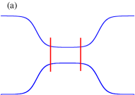
Let us consider the polarization of the asymptotic states. We will assume that only a few transverse channels are open in the QPC, and in the highest channel, the Fermi energy is close to the top of the barrier. In the asymptotic region, the confinement along $y$ becomes infinitely wide as the channel smoothly connects to the 2D leads, Fig.2a, so that for scattering states at the Fermi energy,

$$p_{y}^{2},U(x)\rightarrow 0$$ (3)

$$p_{x}\rightarrow p_{F}$$

and hence

$$H(x\rightarrow\pm\infty)=\frac{p_{x}^{2}}{2m}-\frac{1}{2}|g\mu_{B}|\vec{B}_{\text{eff.}}\cdot\vec{\sigma}\ ,$$ (4)

where we have absorbed the total spin-dependent interactions into an effective magnetic field

$$\vec{B}_{\text{eff.}}(\pm\infty)=\vec{B}+\frac{b^{6c6c}_{41}p_{F}p_{z}^{2}}{\frac{1}{2}|g\mu_{B}|}\hat{x}\ .$$ (5)

For the purpose of numerical calculations which we present in Section IV, we assume that the value of $p_{z}$ corresponds to an infinite well with width 10nm and set the Fermi energy equal to 5meV. Based on the values given in WinklerBook , we may estimate the effective Dresselhaus field to be

$$B_{D}=\frac{b^{6c6c}_{41}p_{F}p_{z}^{2}}{\frac{1}{2}|g^{*}\mu_{B}|}=16\text{T}\ .$$ (6)

When the external magnetic field is directed along $y$, the asymptotic form of the Hamiltonian will form a spin basis with polarization the $x-y$ plane, and for fields in the typical experimental range, $B<\text{15T}$, the orientation of spin for an electron incident on the barrier will always be significantly tilted towards the $x$-direction. The angle $\theta$ between spin and the $y$-direction is close to 60⁰ for fields of the order of 10T, and can be tuned to nearly 90⁰ by reducing the field to 1T. Near the centre of the QPC, where the electrostatic potential is maximum, the longitudinal momentum vanishes semiclassically, and the total effective magnetic field is directed perpendicular to the wire, so that $\theta$ switches to zero, Fig.1b.

Spin dynamics is nonadiabatic when the effective magnetic field changes sufficiently rapidly and hence the Landau-Zener parameter is not small com1 ,

$$\delta_{s}=\frac{1}{g^{*}\mu_{B}B_{\text{eff.}}^{2}}|\frac{dB_{\text{eff.}}}{dt}|\gtrsim 1$$ (7)

Let us assume that the effective field $B_{\text{eff.}}$ switches by an angle of $60^{0}$ over a typical time $\Delta t=\frac{\Delta x}{v_{F}}$ corresponding to the distance $\Delta x$ over which the electrostatic potential is rapidly varying. Then expressing $\delta_{s}$ in terms of the Fermi energy $\epsilon_{F}\approx 5\text{meV}$, we find

$$\delta_{s}=\frac{1}{g\mu_{B}|B_{\text{eff.}}|}\frac{v_{F}}{\Delta x}\cos 60^{0}=\frac{1}{2}\frac{\epsilon_{F}}{g\mu_{B}|B_{\text{eff.}|}}\frac{1}{\Delta xk_{F}}\ .$$ (8)

Taking $|B_{\text{eff.}}|\approx 10\text{T}$, we find that $\frac{\epsilon_{F}}{g\mu_{B}|B_{\text{eff.}}|}\approx 20$, so in order to go to the nonadiabatic regime one needs the following,

$$\Delta xk_{F}\ll 10\rightarrow\Delta x\lesssim 0.1\mu\text{m}\ .$$ (9)

For a single barrier, the conductance is proportional to the transmission coefficient averaged over incident spin polarizations and is therefore insensitive to spin dynamics com2 . In a geometry consisting of two barriers, however, non-trivial precession between the barriers may be observed due to interference between spin in counterpropagating directions in the region between the barriers. This effect exists only when the external field is perpendicular to the contact, since for a parallel field, the total effective field and therefore spin will be constant in direction, either parallel or antiparallel to the contact with no mixing between the spin modes. Similarly, when the external field is perpendicular but sufficiently large to dominate the effective field in the asymptotic region, the effective field will rotate by a sufficiently small angle that the electron will adiabatically follow a single spin channel throughout the motion. This illustrates why the structure of transmission in the double barrier is strongly sensitive to the nonadiabaticity of the spin motion.

III Adiabatic transmission through a double barrier

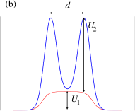
Let us first consider the spin-independent transmission problem for a system consisting of two QPCs in series, with the potential as shown in Fig.2b. We shall assume that the inelastic mean free path exceeds the system size, so that motion is ballistic.

We model the conductance in the Landauer-Büttiker picture ButtikerQPC ; Landauer by one-dimensional scattering in the presence of two barriers separated by a distance $d$. Recall that for a single barrier located at the origin we have a scattering state corresponding to an electron emerging on the right with unit amplitude,

$$\psi(x\gg 0)=e^{ikx}$$ (10)

$$\psi(x\ll 0)=t_{11}e^{ikx}+t_{21}e^{-ikx}\ .$$

Near the top the barrier has parabolic shape

$$U(x\approx 0)=U(0)-\frac{m\omega_{x}^{2}x^{2}}{2}$$ (11)

and hence $T$-matrix elements $t_{11},t_{21}$ are given by the connection formulas of the parabolic cylinder functions AbramowitzStegun ,

$$T=\left(\begin{array}[]{cc}t_{11}&t_{21}^{*}\\ t_{21}&t_{11}^{*}\end{array}\right)=$$ (14)

$$\left(\begin{array}[]{cc}i\sqrt{1+e^{-\frac{2\pi\epsilon}{\omega_{x}}}}&ie^{-\frac{\pi\epsilon}{\omega_{x}}-i\text{Arg}(\frac{1}{2}-\frac{i\epsilon}{\omega_{x}})}\\ -ie^{-\frac{\pi\epsilon}{\omega}+i\text{Arg}(\frac{1}{2}-\frac{i\epsilon}{\omega_{x}})}&-i\sqrt{1+e^{-\frac{2\pi\epsilon}{\omega_{x}}}}\end{array}\right)\ ,$$ (17)

where $\epsilon$ is the Fermi energy relative to the height of the barrier,

$$\epsilon=\varepsilon_{F}-U(0)\ .$$ (18)

Note that for the spinless case the T-matrix has dimension 2$\times$2. The transmission probability through the single barier is

$$P(\epsilon)=\frac{1}{|t_{11}|^{2}}$$ (19)

The $T$-matrix for transmission through the double barrier potential is given by the product of two $T$-matrices for a single barrier with the phase evolution operator,

$$T^{\prime}=T\left(\begin{array}[]{cc}e^{ikd}&0\\ 0&e^{-ikd}\end{array}\right)T\ .$$ (22)

Since the state emerging on the right has unit amplitude, the transmission probability is simply given by

$$P(\epsilon)=\frac{1}{|t^{\prime}_{11}|^{2}}=\frac{1}{|t_{11}^{2}+|t_{21}|^{2}e^{2ikd}|^{2}}=$$ (23)

$$\frac{1}{|1+e^{-\frac{2\pi\epsilon}{\omega_{x}}}(1-e^{2ikd})^{2}|^{2}}$$

and exhibits resonant transmission peaks at $kd=n\pi$ corresponding to standing waves between the barriers.

Initial measurements of the quantised conductance in a DQPC by D. Wharam, et al Wharam did not reveal resonant structure, although it was later reported by Y. Hirayama and T. Saku that resonances became visible when the separation between the two QPCs was reduced to 0.2$\mu$m Hirayama . Since the authors claim that the inelastic mean free path exceeds the size of the device, the loss of interference does not originate from inelastic decoherence, but is rather due to the fact that the region between the QPCs consists of a wide cavity in which a large number of transverse modes are permitted. Here, the loss of phase memory may be attributed to the exchange of phase among the large number of transverse modes and is therefore a purely single particle effect. In other words, phase memory is lost in the course of chaotic motion in the 2D region separating the QPCs.

In order to observe the transmission interference peaks, it is necessary to suppress mixing between transverse modes in the region between the barriers, which is equivalent to the statement that the evolution of the standing wave along $y$ must be adiabatic, and therefore the Landau-Zener condition must be satisfied for the transverse adiabatic parameter.

$$\delta_{t}=\frac{1}{\omega_{y}^{2}}\frac{d\omega_{y}}{dt}=\frac{1}{\omega_{y}^{2}}\frac{p_{x}}{m}\frac{d\omega_{y}}{dx}\ll 1\ ,$$ (24)

where we have assumed a parabolic confinement in the $y$-direction with level spacing $\omega_{y}$. For a typical QPC, the oscillator frequency $\omega_{y}$ is maximum at the centre of the wire ($x=0$), but decreases smoothly to zero in the two-dimensional leads. Modelling the transverse confinement by a gaussian,

$$\omega_{y}(x)=\omega_{0}e^{-\kappa^{2}x^{2}}\ ,$$ (25)

where $\kappa$ is the barrier width, which is of order $\kappa\sim 1\mu m$, we find

$$\delta_{t}=-\frac{2\kappa^{2}xp_{x}}{m\omega_{0}}e^{\kappa^{2}x^{2}}\ .$$ (26)

Away from the contact, $x\rightarrow\pm\infty$, the adiabatic parameter diverges due to the collapsing of the transverse level spacing. We therefore see that a loss of interference is unavoidable in a system consisting of two QPCs which are separated by a wide cavity. Hereafter we consider an interferometer which consists of a 1D channel of fixed width in which a double barrier is formed by an additional potential $U_{2}(x)$ (i.e. an inhomogeneous shift of the 1D band bottom) rather than by the energy of transverse confinement. In the region between the barriers, the 2D potential has the form

$$U_{2D}(x,y)=\frac{m\omega_{y}^{2}y^{2}}{2}+U_{2}(x)\ ,$$ (27)

and the oscillator frequency $\omega_{y}$ is approximately constant inside the channel, so that an electron remains in a single transverse mode during motion between the barriers.

The potential (27) can be manufactured, for example, by a rectangular split gate in the plane of the 2DEG, with two thin wires placed perpendicular to the channel in a plane separated from the 2DEG by an insulating layer, Fig. 2a. When there is a bias between the wires in the upper layer and the 2DEG, a smooth electrostatic potential will be formed in the channel below. The 1D channel is quantized into oscillator levels, with the 1D effective potential being

$$U(x)=U_{1}(x)+U_{2}(x)$$ (28)

$$U_{1}(x)=\omega_{y}(x)(n+\frac{1}{2})$$

where $n$ is the transverse oscillator level. We also suppose that the channel is not near pinch-off, so that the additional barrier $U_{2}(x)$ may be made high without depleting the channel. As long as the wires are placed inside the edges of the point contacts, the level spacing will be constant, and transport between the potential barriers in the channel created by the wires will be adiabatic.

IV Resonant transmission of spin

We expect that the presence of nonadiabatic spin precession will result in an observable change in the conductance when the distance between the barriers is of the order of the length of a spin cycle,

$$l_{s}=\frac{2\pi v_{F}}{\frac{1}{2}g^{*}\mu_{B}B}=\frac{\epsilon_{F}}{\frac{1}{2}g^{*}\mu_{B}B}\frac{2\pi}{k_{F}}=\frac{\epsilon_{F}}{\frac{1}{2}g^{*}\mu_{B}B}\lambda=1.2\mu\text{m}$$ (29)

when the Fermi energy is 5meV. We reiterate that to observe the effect of nonadiabaticity on the conductance, it is necessary to have $\delta_{s}\gg 1$ at the barriers, and $\delta_{t}\ll 1$ everywhere in the region between the barriers.

Due to the small $g$-factor of electrons, the longitudinal oscillator frequency $\omega_{x}$ must be sufficiently small in order to resolve the Zeeman splitting in the external magnetic field, and we take the value of $\omega_{x}=0.19\text{meV}$ corresponding to a gaussian half-width of $0.4\mu$m. When $d<2\mu$m, we find that the potentials of the two barriers overlap, reducing the velocity and hence the magnitude of the Dresselhaus effective field between the barriers. In principle, it is possible to engineer a system with $d=1\mu$m while maintaining a large Dresselhaus field by using a third wire above the point contact which is positively biased to create a deeper cavity between the barriers. In our numerics, however, we will consider only the simpler geometry consisting of two wires in a plane above the point contact, and take a larger separation, $d=2\mu$m, see Fig.2b. The 1D Hamiltonian is

$$H=\frac{p_{x}^{2}}{2m}+U(x)-\alpha p_{x}\sigma_{x}-\frac{1}{2}g^{*}\mu_{B}\vec{B}\cdot\vec{\sigma}\ ,$$ (30)

where $\alpha=b^{6c6c}_{41}p_{z}^{2}$ and we have dropped the term proportional to $p_{y}^{2}$, which does not qualitatively influence the result. When the external magnetic field is directed along $x$, the Hamiltonian becomes diagonal in the basis of states with spin aligned along the contact, and the transmission coefficients for the spin-up and spin-down channels are simply given by the sum of two zero-field transmission coefficients shifted relative to one another by the Zeeman splitting $|g^{*}\mu_{B}B|$; the Dresselhaus interaction does not have any effect. For the perpendicular orientation of the external field, the behaviour of the transmission coefficient is expected to be significantly more complex due to nonadiabaticity, since the Hamiltonian does not decouple in any locally defined basis.

We have solved the scattering problem using numerical integration of the Schrodinger equation via the fourth-order Adams-Moulton method, which was required due to the presence of the first power of momentum in the Hamiltonian (30). The conductance due to a single transverse channel, according to the Landauer formula, is related to the $2\times 2$ spin-dependent transmission amplitude $A$ by

$$G=\frac{e^{2}}{h}P(\epsilon)\ ,\ \ \ P(\epsilon)=\text{tr}A^{\dagger}A\ .$$ (31)

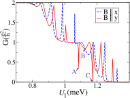
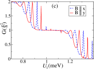
The calculated conductance for fields 5T, 10T, and 15T in the parallel and perpendicular orientations is plotted in Fig.3 versus $U_{1}$, which is the contribution to the effective 1D potential which is constant between the barriers defined in (28).

Figure 3: (Color online). The conductance (units of $\frac{e^{2}}{h}$) of the DQPC interferometer ($d=2\mu$m) versus the constant contribution to the potential $U_{1}$ defined in (28). The conductance is plotted for three values of the external magentic field, (a)5T, (b) 10T, (c) 15T, parallel (dotted line) and perpendicular (solid line) to the contact. The arrows in (b) refer to the three plots in Fig.5.

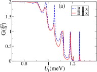
The difference between the resonant structure observed for the two field orientations is due to the Dresselhaus interaction. Whereas the interaction does not influence the resonant pattern for the case of parallel field, it does so for the perpendicular orientation. We plot the field dependence of the resonant peak positions in Fig.4.

Figure 4: (Color online). Position of the magnetoconductance peaks as a function of magnetic field for parallel (a) and perpendicular (b) orientations of the fields.

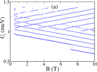
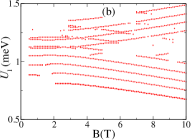
For a parallel applied field, the positions of the peaks are shifted linearly in the magnetic field, with slope equal to the magnetic moment $\pm\frac{1}{2}g^{*}\mu_{B}$ and opposite spins exhibiting shifts in opposite directions. The situation for perpendicular field, however, is markedly different: in the low field regime the positions of the peaks depend non-linearly on the applied field and evolve into straight lines with slope $\pm\frac{1}{2}g^{*}\mu_{B}$ as the field is increased. In the high field regime, the positions of the peaks are still off-set relative to those in the parallel orientation, even though spin dynamics is becoming adiabatic. This is due to the fact that the Dresselhaus interaction not only induces a non-abelian phase when nonadiabatic precession occurs, but also contributes to the abelian phase even in the adiabatic regime, so that the peaks in high field remain offset due to the accumulation of a dynamical phase in the scattering regions in which spin undergoes significant precession.

In addition to the non-linear shift in the positive transmission resonant peaks we observe a novel feature in the regime where nonadiabaticity of the spin motion is strong, these are the negative resonances appearing on the middle plateau. The negative resonances marked by letters (A) and (C) are evident in Fig.3b at 10T, and are suppressed as the magnetic field is increased into the adiabatic regime. Recall that in the spinless situation, sharp peaks appear in the transmission corresponding resonant transparency at energies where a quasi-bound state exists between the barriers. It is clear that appearance of negative peaks corresponding to resonant enhancement of reflection cannot exist for parallel fields, and is therefore closely tied to non-trivial spin dynamics. In Fig.5 we display the electron wave functions corresponding to energies (A), (B), and (C) marked in the conductance plot Fig.3b.

Figure 5: The probability $|\psi|^{2}$ plotted on the same scale at three values of $U_{1}$, corresponding to the two negative resonant cases (A,C) and one off-resonant case (B) indicated in Fig.3b. The wavefunction is strongly enhanced between the barriers at negative resonances, clearly demonstrating the existence of quasi-bound states.

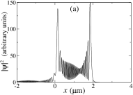
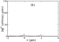
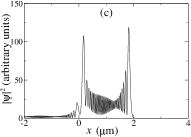
We observe that the wavefunction at energies corresponding to negative resonances (A) and (C) is strongly enhanced between the barriers signalling the presence of a quasi-bound state at the two resonant energies. We reiterate that these states appear at 10T and are associated with a suppression in the transmission. At high magnetic field the states gradually disappear; they are evident only vestigially at 15T, Fig.3c.

Practically, the non-linear field dependence of the splitting of ususal (“positive”) transmission resonances shown in Figs.  3 and  4 might provide a robust way to probe and to measure the Dresselhaus and the Rashba interactions. On the other hand observation of the negative resonances might be a challenge because of their relatively small spectral weight (we observe numerically that the negative resonances are more pronounced for heavy holes than for electrons). On the other hand the negative resonances are a qualitatively new feature related to the non-abelian and non-adiabatic spin dynamics and we shall explain the physical mechanism behind these features in the next section.

V The physical mechanism for negative resonances.

Let us consider the region very near the top of the barrier, in which $p_{x}\approx 0$. Since the external magnetic field is dominant near the barrier, the scattering of a state which is incident on the single barrier is completely described by the spin-dependent $T$-matrix for a single parabolic barrier with constant magnetic field,

$$\hat{T}=\left(\begin{array}[]{cc}\hat{t}_{11}&\hat{t}_{12}\\ \hat{t}_{21}&\hat{t}_{22}\end{array}\right)\ .$$ (34)

Hereafter we indicate the explicit inclusion of spin by the hat above the $T$-matrix; the dimension of $\hat{T}$ is hence 4$\times$4. The $2\times 2$ matrices $\hat{t}_{ij}$ are diagonal in the basis of states with spin directed along the external field $\vec{B}$,

$$\hat{t}_{ij}=\left(\begin{array}[]{cc}t_{ij}(\epsilon+\epsilon_{B})&0\\ 0&t_{ij}(\epsilon-\epsilon_{B})\end{array}\right)\ .$$ (37)

Here we have written $\epsilon_{B}=|\frac{1}{2}g^{*}\mu_{B}B|$ and the spin-independent matrix elements $t_{ij}(\epsilon)$ were given in Eq. (14). In the situation where $2\epsilon_{B}\gg\omega_{x}$, the Zeeman splitting may be clearly resolved, a middle plateau exists, and for energies lying on this plateau, each barrier acts as a spin filter, preferentially reflecting spins which are aligned with the magnetic field and transmitting spins which are anti-aligned.

Away from the potential barriers, the electron momentum is large and hence it is possible to perform a Born-Oppenheimer separation of orbital and spin motion. Writing the wave-function as

$$\psi(x)=e^{i\int{kdx}}\chi(x)\ ,$$ (38)

where $\chi$ is a spinor and

$$k=\sqrt{2m(\epsilon-U)}\ ,$$ (39)

we find that $\chi$ obeys the following Schrodinger equation

$$i\frac{d\chi}{d\tau}=-(\epsilon_{B}\sigma_{y}+\alpha k\sigma_{x})\chi\ .$$ (40)

Here $\tau$ is an effective time defined by

$$\frac{k}{m}\frac{d}{dx}=\frac{d}{d\tau}\ .$$ (41)

When deriving Eq. (40) from Eq. (30) one has to remember that between the barriers, $\alpha\ll\frac{k}{m}$. The solution $\chi(\tau)$ may be written in terms of the SU(2) evolution operator $U(\tau)$,

$$\chi(\tau)=U(\tau)\chi(0)$$ (42)

We have used the same letter for the evolution operator as for the potential, however the meaning should be clear.

In the region between the two barriers, the wave-function consists of counterpropagating waves which carry precessing spin. The spins which propagate in opposite directions are related by an operation corresponding to the reversal of ’effective time’, which differs from the usual time-reversal operator in that $\sigma_{x}$ does not change sign since the $x$-component of the effective magnetic field $\alpha p_{x}$ is also reversed. It is therefore necessary to augment the time-reversal operator by a rotation of $\pi$ about the $y$-axis. The unitary evolution operator then obeys the relation

$$U(-\tau)=e^{-\frac{i\pi\sigma_{y}}{2}}U(\tau)^{\dagger}e^{\frac{i\pi\sigma_{y}}{2}}\ .$$ (43)

Since the region in which the electron sees a relatively constant magnetic field extends over a large number of de Broglie wavelengths, while the scattering region consists of a small number of de Broglie wavelengths, the $T$-matrix for the complete process is simply given by the product of the individual $T$-matrices at each barrier with the matrix describing phase and spin evolution between the barriers,

$$\hat{T}^{\prime}=\hat{T}\left(\begin{array}[]{cc}e^{i\Phi}U(\tau)&0\\ 0&e^{-i\Phi}U(-\tau)\end{array}\right)\hat{T}$$ (46)

where $e^{i\Phi}$ is an abelian phase and

$$U(\tau)=\left(\begin{array}[]{cc}\alpha&-\beta^{*}\\ \beta&\alpha^{*}\end{array}\right),\ \ \ U(-\tau)=\left(\begin{array}[]{cc}\alpha^{*}&-\beta\\ \beta^{*}&\alpha\end{array}\right)$$ (51)

The spin-dependent 2$\times$2 transmission amplitude is given by

$$A=\hat{t}_{11}^{\prime-1}=(\hat{t}_{11}e^{i\Phi}U(\tau)\hat{t}_{11}+\hat{t}_{12}e^{-i\Phi}U(-\tau)\hat{t}_{21})^{-1}$$ (52)

When the energy lies on the middle plateau, $\epsilon+\epsilon_{B}\approx\epsilon_{B}\gg 0,\epsilon-\epsilon_{B}\approx-\epsilon_{B}\ll 0$, we obtain, making use of the explicit forms (14)

$$\hat{t}^{\prime}_{11}\approx$$

$$-e^{i\Phi}\left(\begin{array}[]{cc}1&0\\ 0&\sqrt{1+e^{2\pi\epsilon_{B}/\omega_{x}}}\end{array}\right)\left(\begin{array}[]{cc}\alpha&-\beta^{*}\\ \beta&\alpha^{*}\end{array}\right)\left(\begin{array}[]{cc}1&0\\ 0&\sqrt{1+e^{2\pi\epsilon_{B}/\omega_{x}}}\end{array}\right)+e^{-i\Phi}\left(\begin{array}[]{cc}0&0\\ 0&e^{\pi\epsilon_{B}/\omega_{x}}\end{array}\right)\left(\begin{array}[]{cc}\alpha^{*}&-\beta\\ \beta^{*}&\alpha\end{array}\right)\left(\begin{array}[]{cc}0&0\\ 0&e^{\pi\epsilon_{B}/\omega_{x}}\end{array}\right)$$ (65)

$$=\left(\begin{array}[]{cc}-\alpha e^{i\Phi}&-\beta^{*}e^{\pi\epsilon_{B}/\omega_{x}}e^{i\Phi}\\ \beta e^{\pi\epsilon_{B}/\omega_{x}}e^{i\Phi}&(\alpha e^{-i\Phi}-\alpha^{*}e^{i\Phi})e^{2\pi\epsilon_{B}/\omega_{x}}-\alpha^{*}e^{i\Phi}\end{array}\right)\ .$$ (68)

The spin-dependent transmission amplitude is

$$A=\frac{e^{-i\Phi}}{|\alpha|^{2}+e^{2\pi\epsilon_{B}/\omega_{x}}(1-\alpha^{2}e^{-2i\Phi})}\left(\begin{array}[]{cc}(\alpha e^{-2i\Phi}-\alpha^{*})e^{2\pi\epsilon_{B}/\omega_{x}}-\alpha^{*}&-\beta^{*}e^{\pi\epsilon_{B}/\omega_{x}}\\ \beta e^{\pi\epsilon_{B}/\omega}&-\alpha\end{array}\right)$$ (71)

The off-diagonal matrix elements $A_{12},A_{21}$ correspond to transmission with spin-flip. The conductance is given by

$$G=\frac{e^{2}}{h}\text{tr}AA^{\dagger}=\frac{e^{2}}{h}(|A_{11}|^{2}+|A_{12}|^{2}+|A_{21}|^{2}+|A_{22}|^{2})$$ (72)

We may immediately identify the off-resonant situation when the exponential factor $e^{2\pi B/\omega}$ is dominant, so that the transmission amplitude and probabilty are of the form

$$A=e^{-i\Phi}\frac{\alpha e^{-2i\Phi}-\alpha^{*}}{(1-\alpha^{2}e^{-2i\Phi})}\left(\begin{array}[]{cc}1&0\\ 0&0\end{array}\right)$$ (75)

$$P(\epsilon)=|\alpha|^{2}\approx 1\ .$$ (76)

which corresponds to the filtering of spin at each barrier.

At a usual “positive” resonance

$$1-\alpha^{2}e^{-2i\Phi}=0\rightarrow\alpha=e^{i(\Phi+n\pi)}\ .$$ (77)

This implies that $|\alpha|=1$, $\beta=0$. Hence

$$A=\frac{e^{-i\Phi}}{|\alpha|^{2}}\left(\begin{array}[]{cc}-\alpha^{*}&0\\ 0&-\alpha\end{array}\right)$$ (80)

$$P(\epsilon)=2\ .$$ (81)

At a “negative” resonance we need to satisfy the following conditions

$$\alpha e^{-2i\Phi}-\alpha^{*}=0$$

$$1-\alpha^{2}e^{-2i\Phi}\neq 0\ .$$ (82)

This is possible only if $\alpha=|\alpha|e^{i(\Phi+n\pi)}$ and $|\alpha|<1$. The phase condition is the same as that for the positive resonace, Eq. (77). However, $|\alpha|<1$ is possible only in a nonadibatic case. In this case we have

$$A=\frac{e^{-i\Phi}}{|\beta|^{2}e^{2\pi\epsilon_{B}/\omega_{x}}}\left(\begin{array}[]{cc}-\alpha^{*}&-\beta^{*}e^{\pi\epsilon_{B}/\omega_{x}}\\ \beta e^{\pi\epsilon_{B}/\omega_{x}}&-\alpha\end{array}\right)$$ (85)

$$P(\epsilon)=e^{-2\pi\epsilon_{B}/\omega_{x}}\ .$$ (86)

We see that in order to obtain a negative resonance it is necessary for spin to precess non-trivially, so that a lower spin component develops over the course of the trajectory. When motion is significantly nonadiabatic, the lower component of spin may undergo resonant enhancement, leading to suppression of transmission. When the parameters are driven deeper into the adiabatic regime, we find that the resonant behaviour can reverse to become a more common positive resonance, which explains how the negative spike marked (A) in Fig.3b appears as a small positive “bump” on the middle plateau in panel (c) of the same figure.

In order to observe a negative resonance, it is necessary that nonadiabatic spin dynamics persist into the high-field regime, since the Zeeman splitting must be sufficient large to create a middle plateau in which one spin channel is filtered. This requires that the Zeeman splitting be larger than the longitudinal oscillator frequency, $g^{*}\mu_{B}B>\omega_{x}$, while remaining significantly smaller than the Dresselhaus interaction. While this can be accomplished by making the parabolic barrier wider, this would also require the distance between barriers to be increased, which is a sensitive issue since the size of the system may be required to exceed the ballistic mean free path. We therefore expect that while the non-linear splitting of peaks shown in Figs.  3 and  4 should be confirmed experimentally with relative ease, realization of the negative resonances may provide a challenge.

VI Conclusion

We suggest a spin-orbit interferometer consisting of two QPCs connected in series. It is shown that due to the Dresselhaus spin-orbit interaction the spin dynamics in the interferometer is nonadiabatic in presence of an external magnetic field. As a result of this nonadiabaticity the positions of the resonant peaks in the transmission are sensitive to the direction of the magnetic field and the value of the Dresselhaus interaction. This effect could be used to directly measure the size of the Dresselhaus interaction in a ballistic channel. While we performed our calculations for an electron system with the Dresselhaus interaction, it is clear that the same effect exists generically for holes and for the Rashba spin-orbit interaction.

We thank U. Zuelicke, A. R. Hamilton and A. I. Milstein for stimulating discussions.

References

- (1) S. Datta and B. Das, Appl. Phys. Lett”, 56, 665 (1990).
- (2) M.I. D’yakonov and V.I. Perel’, Zh. Eksp. Teor. Fiz. 60, 1954, (1971). [Sov. Phys. JETP 33, 1053 (1971)]
- (3) M.I. D’yakonov and V.I. Perel’, Fiz. Tverd. Tela (Leningrad), 13, 3581 (1971). [Sov. Phys. Solid State 13, 3023 (1972)]
- (4) R.J. Elliott, Phys. Rev., 96, 266 (1954).
- (5) Y. Yafet, Solid State Physics, vol.14”, Academic Press, New York, 1963.
- (6) M. Eto, T. Hayashi, Y. Kurotani, and H. Yokouchi, Phys. Stat. Sol. C, 3, 4168 (2006).
- (7) M.M. Gelabert, D. Sanchez, R. Lopez, and L. Serra, Phys. Stat. Sol. C”, 6, 2123 (2009).
- (8) M. Governale and U. Zulicke, Journal of Superconductivity: Incorporating Novel Magnetism, 16, 257, (2003).
- (9) M. Governale and U. Zulicke, Solid State Commun., 131, 581 (2004).
- (10) T. Kita, T. Kakegawa, M. Akabori, and S. Yamada, Physica E, 22, 464, (2004).
- (11) G. Liu and G. Zhou, J. Appl. Phys., 101, 063704 (2007).
- (12) X. Xiao, X. Li and Y. Chen, Phys. Lett. A, 373, 4489 (2009).
- (13) R. Winkler, Spin-Orbit Coupling Effects in Two-Dimensional Electron and Hole Systems, Springer Tracts in Modern Physics. Vol 191, 2003.
- (14) L. Meier, G. Salis, I. Shorubalko, E. Gini, S. Schön, and K. Ensslin, Nature Physics, 3, 650 (2007).
- (15) Throughout we set .
- (16) This conclusion was also confirmed numerically via explicit calculation of the transmission coefficient.
- (17) M. Buttiker, Phys. Rev. B, 41, 7906, (1989).
- (18) R. Landauer, J. Phys.: Condens. Matter, 1, 8099 (1989).
- (19) M. Abramowitz and I.A. Stegun”, Handbook of Mathematical Functions, Dover Publications, 1965.
- (20) D. A. Wharam, T. J. Thornton, R. Newbury, M. Pepper, H. Ahmed, J. E. F. Frost, D. G. Hasko, D. C. Peacock, D. A. Ritchie, and G. A. C. Jones, J. Phys. C, 21, L209 (1988).
- (21) Y. Hirayama and T. Saku, Phys. Rev. B, 41, 2927 (1990).