Stability switching at transcritical bifurcations of solitary waves in generalized nonlinear Schrödinger equations

Abstract

Linear stability of solitary waves near transcritical bifurcations is analyzed for the generalized nonlinear Schrödinger equations with arbitrary forms of nonlinearity and external potentials in arbitrary spatial dimensions. Bifurcation of linear-stability eigenvalues associated with this transcritical bifurcation is analytically calculated. Based on this eigenvalue bifurcation, it is shown that both solution branches undergo stability switching at the transcritical bifurcation point. In addition, the two solution branches have opposite linear stability. These stability properties closely resemble those for transcritical bifurcations in finite-dimensional dynamical systems. This resemblance for transcritical bifurcations contrasts those for saddle-node and pitchfork bifurcations, where stability properties in the generalized nonlinear Schrödinger equations differ significantly from those in finite-dimensional dynamical systems. The analytical results are also compared with numerical results, and good agreement is obtained.

1 Introduction

The generalized nonlinear Schrödinger equations considered in this article are a large class of Schrödinger-type equations which contain arbitrary forms of nonlinearity and external potentials in arbitrary spatial dimensions. This class of equations are physically important since they include theoretical models for nonlinear light propagation in refractive-index-modulated optical media [2, 3] and for atomic interactions in Bose-Einstein condensates loaded in magnetic or optical traps [4] as special cases. Given their physical importance, these equations have been heavily studied in the physical and mathematical communities. These equations admit a special but important class of solutions called solitary waves, which are spatially localized and temporally stationary structures of the system. These solitary waves exist for continuous ranges of the propagation constant. At special values of the propagation constant and under certain conditions, bifurcations of solitary waves can occur. Indeed, various solitary wave bifurcations in these equations have been reported. Examples include saddle-node bifurcations (also called fold bifurcations) [3, 5, 6, 7, 8, 9, 10], pitchfork bifurcations (sometimes called symmetry-breaking bifurcations) [8, 11, 12, 13, 14, 15], and transcritical bifurcations [16]. These three types of bifurcations have also been classified in [16], where analytical conditions for their occurrence were derived.

Stability of solitary waves near these bifurcations is an important issue. In finite-dimensional dynamical systems, stability of fixed-point branches near these bifurcations is well known [17]. However, as was explained in [10, 18], those stability results from finite-dimensional dynamical systems cannot be extrapolated to the generalized nonlinear Schrödinger equations. Thus this stability in the generalized nonlinear Schrödinger equations has to be studied separately. For saddle-node bifurcations of solitary waves, this stability question has been analyzed in [9, 10]. It was shown that no stability switching takes place at a saddle-node bifurcation, which is in stark contrast with finite-dimensional dynamical systems where stability switching generally takes place [17]. For pitchfork bifurcations of solitary waves, this stability has been analyzed in [12, 13, 15, 18]. It was shown that this stability possesses novel features which have no counterparts in finite-dimensional dynamical systems as well. For instance, the base and bifurcated branches of solitary waves (on the same side of a pitchfork bifurcation point) can be both stable or both unstable [15, 18], which contrasts finite-dimensional dynamical systems where the bifurcated fixed-point branches generally have the opposite stability of the base branch [17]. For transcritical bifurcations of solitary waves, the stability question is still open.

In this paper, we analyze the linear stability of solitary waves near transcritical bifurcations in the generalized nonlinear Schrödinger equations. Our strategy is to analytically calculate bifurcations of linear-stability eigenvalues from the origin when the transcritical bifurcation occurs. Based on this eigenvalue bifurcation and assuming no other instabilities interfere, linear stability of solitary waves near the transcritical bifurcation point is then obtained. We show that both solution branches undergo stability switching at the transcritical bifurcation point. In addition, the two solution branches have opposite linear stability. These stability properties closely resemble those for transcritical bifurcations in finite-dimensional dynamical systems. Thus, among the three major bifurcations (i.e., saddle-node, pitchfork and transcritical bifurcations), the transcritical bifurcation is the only one where stability properties in the generalized nonlinear Schrödinger equations closely resemble those in finite-dimensional dynamical systems. In the end, we also present a numerical example which confirms our analytical predictions.

2 Stability results for transcritical bifurcations of solitary waves

We consider the generalized nonlinear Schrödinger (GNLS) equations with arbitrary forms of nonlinearity and external potentials in arbitrary spatial dimensions. These equations can be written as

$$iU_{t}+\nabla^{2}U+F(|U|^{2},\mathbf{x})U=0,$$ (2.1)

where $\nabla^{2}=\partial^{2}/\partial x_{1}^{2}+\partial^{2}/\partial x_{2}^{2}+\cdots+\partial^{2}/\partial x_{N}^{2}$ is the Laplacian in the $N$-dimensional space $\textbf{x}=(x_{1},x_{2},\cdots,x_{N})$, and $F(\cdot,\cdot)$ is a general real-valued function which includes nonlinearity as well as external potentials. These GNLS equations include the Gross-Pitaevskii equations in Bose-Einstein condensates [4] and nonlinear light-transmission equations in linear potentials and nonlinear lattices [2, 3, 19, 20] as special cases. Notice that these equations are conservative and Hamiltonian.

For a large class of nonlinearities and potentials, this equation admits stationary solitary waves

$$U(\mathbf{x},t)=e^{i\mu t}u(\mathbf{x}),$$ (2.2)

where $u(\mathbf{x})$ is a real and localized function in the square-integrable functional space which satisfies the equation

$$\nabla^{2}u-\mu u+F(u^{2},\mathbf{x})\hskip 1.42271ptu=0,$$ (2.3)

and $\mu$ is a real-valued propagation constant. In these solitary waves, $\mu$ is a free parameter, and $u(\mathbf{x})$ depends continuously on $\mu$. Under certain conditions, these solitary waves undergo bifurcations at special values of $\mu$. Three major types of bifurcations, namely, saddle-node, pitchfork and transcritical bifurcations, have been classified in [16]. In addition, linear stability of solitary waves near saddle-node and pitchfork bifurcations has been determined in [9, 10, 12, 13, 15, 18]. In this paper, we determine the linear stability of solitary waves near transcritical bifurcations in the GNLS equations (2.1).

A transcritical bifurcation in the GNLS equations (2.1) is where there are two smooth branches of solitary waves $u^{\pm}(\mathbf{x};\mu)$ which exist on both sides of the bifurcation point $\mu=\mu_{0}$, and these two branches cross each other at $\mu=\mu_{0}$. A schematic solution-bifurcation diagram of transcritical bifurcations is shown in Fig. 1(a). Analytical conditions for transcritical bifurcations in Eq. (2.1) were derived in [16]. To present these conditions, we introduce the linearization operator of Eq. (2.3),

$$L_{1}=\nabla^{2}-\mu+\partial_{u}[F(u^{2},\mathbf{x})u],$$ (2.4)

which is a linear Schrödinger operator. We also introduce the standard inner product of functions,

$$\langle f,g\rangle=\int_{-\infty}^{\infty}f^{*}(\mathbf{x})\hskip 1.42271ptg(\mathbf{x})\hskip 1.9919ptd\mathbf{x},$$

where the superscript ‘*’ represents complex conjugation. In addition, we define the power of a solitary wave $u(\mathbf{x};\mu)$ as

$$P(\mu)=\langle u,u\rangle=\int_{-\infty}^{\infty}u^{2}(\mathbf{x};\mu)\hskip 1.9919ptd\mathbf{x},$$

and denote the power functions of the two solitary-wave branches as

$$P_{\pm}(\mu)\equiv\langle u^{\pm}(\mathbf{x};\mu),u^{\pm}(\mathbf{x};\mu)\rangle.$$

If a bifurcation occurs at $\mu=\mu_{0}$, by denoting the corresponding solitary wave and the $L_{1}$ operator as

$$u_{0}(\mathbf{x})\equiv u(\mathbf{x};\mu_{0}),\quad L_{10}\equiv L_{1}|_{\mu=\mu_{0},\ u=u_{0}},$$

then $L_{10}$ should have a discrete zero eigenvalue. This is a necessary condition for all bifurcations. In [16], the following sufficient conditions for transcritical bifurcations were derived. In this derivation, it was assumed implicitly that the function $F(u^{2},\mathbf{x})$ is infinitely differentiable with respect to $u$.

Theorem 1  Assume that zero is a simple discrete eigenvalue of $L_{10}$ at $\mu=\mu_{0}$. Denoting the real localized eigenfunction of this zero eigenvalue as $\psi(\mathbf{x})$, and denoting

$$G(u;\mathbf{x})\equiv F(u^{2};\mathbf{x})u,\quad G_{2}(\mathbf{x})\equiv\partial_{u}^{2}G|_{u=u_{0}},$$ (2.5)

then if

$$\langle u_{0},\psi\rangle=0,\quad\langle G_{2},\psi^{3}\rangle\neq 0,$$

and

$$\Delta\equiv\langle 1-G_{2}L_{10}^{-1}u_{0},,\psi^{2}\rangle^{2}-\langle G_{2},\psi^{3}\rangle\langle G_{2}(L_{10}^{-1}u_{0})^{2}-2L_{10}^{-1}u_{0},\psi\rangle>0,$$

a transcritical bifurcation occurs at $\mu=\mu_{0}$.

Perturbation series for the two solution branches $u^{\pm}(\mathbf{x};\mu)$ near a transcritical bifurcation point were also derived in [16]. It was found that

$$u^{\pm}(\mathbf{x};\mu)=u_{0}(\mathbf{x})+(\mu-\mu_{0})u_{1}^{\pm}(\mathbf{x})+O\{(\mu-\mu_{0})^{2}\},$$ (2.6)

where

$$u_{1}^{\pm}=L_{10}^{-1}u_{0}+b_{1}^{\pm}\psi,$$ (2.7)

and

$$b_{1}^{\pm}\equiv\frac{\langle 1-G_{2}L_{10}^{-1}u_{0},\psi^{2}\rangle\pm\sqrt{\Delta}}{\langle G_{2},\psi^{3}\rangle}.$$ (2.8)

From these perturbation series solutions, power functions $P_{\pm}(\mu)$ near the bifurcation point can be calculated. In particular, one finds that

$$P_{+}^{\prime}(\mu_{0})=P_{-}^{\prime}(\mu_{0}),$$

thus power curves $P_{\pm}(\mu)$ of the two solution branches $u^{\pm}(\mathbf{x};\mu)$ have the same slope at the bifurcation point. Because of this, the two power curves $P_{\pm}(\mu)$ are tangentially touched at a transcritical bifurcation. This feature of the power-bifurcation diagram is shown schematically in Fig. 1(b). Notice that this power-bifurcation diagram of the transcritical bifurcation looks quite different from the solution-bifurcation diagram in Fig. 1(a).

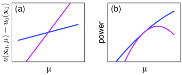
Figure 1: Schematic diagrams of a transcritical bifurcation: (a) solution-bifurcation diagram (plotted is the deviation function $u(\mathbf{x}_{0};\mu)-u_{0}(\mathbf{x}_{0})$ versus $\mu$ at a representative $\mathbf{x}_{0}$ position); (b) power-bifurcation diagram. The same color represents the same solution branch.

The goal of this paper is to analytically determine the linear stability of solitary waves near a transcritical bifurcation point. To study this linear stability, we perturb the solitary waves by normal modes and obtain the following eigenvalue problem (see [3], p176)

$${\cal L}\Phi=\lambda\Phi,$$ (2.9)

where

$${\cal L}=i\left[\begin{array}[]{cc}0&L_{0}\\ L_{1}&0\end{array}\right],\quad\Phi=\left[\begin{array}[]{c}v\\ w\end{array}\right],$$ (2.10)

$$L_{0}=\nabla^{2}-\mu+F(u^{2},\mathbf{x}),$$ (2.11)

and $L_{1}$ has been defined in Eq. (2.4). In the later text, operator ${\cal L}$ will be called the linear-stability operator. If this linear-stability eigenvalue problem admits eigenvalues $\lambda$ whose real parts are positive, then the corresponding normal-mode perturbation exponentially grows, hence the solitary wave $u(\mathbf{x})$ is linearly unstable. Otherwise it is linearly stable. Notice that eigenvalues of this linear-stability problem always appear in quadruples $(\lambda,-\lambda,\lambda^{*},-\lambda^{*})$ when $\lambda$ is complex, or in pairs $(\lambda,-\lambda)$ when $\lambda$ is real or purely imaginary.

Using the operator $L_{0}$, the solitary wave equation (2.3) can be written as

$$L_{0}u=0.$$ (2.12)

In particular, when we denote $L_{0}$ at the bifurcation point as

$$L_{00}\equiv L_{0}|_{\mu=\mu_{0},\ u=u_{0}},$$

then

$$L_{00}u_{0}=0,$$ (2.13)

thus zero is a discrete eigenvalue of $L_{00}$.

The main result of this paper is the following theorem on linear-stability eigenvalues of solitary waves near a transcritical bifurcation point.

Theorem 2  At a transcritical bifurcation point $\mu=\mu_{0}$ in the GNLS equation (2.1), suppose zero is a simple discrete eigenvalue of operators $L_{00}$ and $L_{10}$, and

$$\langle\psi,L_{00}^{-1}\psi\rangle\neq 0,\quad P_{\pm}^{\prime}(\mu_{0})\neq 0,$$ (2.14)

where $\psi$ is the real discrete eigenfunction of the zero eigenvalue in $L_{10}$ (see Theorem 1), then a single pair of non-zero eigenvalues $\pm\lambda$ in the linear-stability operator ${\cal L}$ bifurcate out along the real or imaginary axis from the origin when $\mu\neq\mu_{0}$. In addition, the bifurcated eigenvalues $\lambda^{\pm}$ on the two solution branches $u^{\pm}(\mathbf{x};\mu)$ are given asymptotically by

$$(\lambda^{\pm})^{2}\to\mp\gamma(\mu-\mu_{0}),\quad\mu\to\mu_{0},$$ (2.15)

where the real constant $\gamma$ is

$$\gamma=\frac{\sqrt{\Delta}}{\langle\psi,L_{00}^{-1}\psi\rangle}.$$ (2.16)

A direct consequence of Theorem 2 is the following Theorem 3 which summarizes the qualitative linear-stability properties of solitary waves near a transcritical bifurcation point.

Theorem 3  Suppose at a transcritical bifurcation point $\mu=\mu_{0}$, the solitary wave $u_{0}(\mathbf{x})$ is linearly stable; and when $\mu$ moves away from $\mu_{0}$, no complex eigenvalues bifurcate out from non-zero points on the imaginary axis. Then under the same assumptions of Theorem 2, both solution branches $u^{\pm}(\mathbf{x};\mu)$ undergo stability switching at the transcritical bifurcation point. In addition, the two solution branches have opposite linear stability.

Based on this theorem, schematic stability diagrams for a transcritical bifurcation are displayed in Fig. 2. The stability behavior in Fig. 2(a) (for solution bifurcation) closely resembles that for transcritical bifurcations of fixed points in finite-dimensional dynamical systems [17]. But the power-bifurcation diagram (with stability information) in Fig. 2(b) has no counterpart in finite-dimensional dynamical systems.

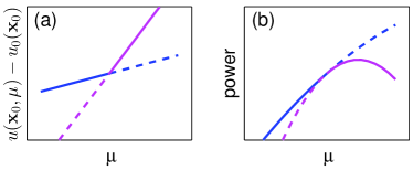
Figure 2: Schematic diagrams of a transcritical bifurcation with stability information indicated: (a) solution-stability diagram; (b) power-stability diagram. The same color represents the same solution branch, and solid (dashed) lines are stable (unstable).

Note that for positive solitary waves in the GNLS equations (2.1), linear-stability eigenvalues are all real or purely imaginary (see [3], Theorem 5.2, p176). In addition, zero is always a simple eigenvalue of $L_{00}$ [21]. In this case, if zero is also a simple eigenvalue of $L_{10}$ and the solitary wave $u_{0}(\mathbf{x})$ at the bifurcation point is linearly stable, then under the generic conditions (2.14), Theorem 3 applies, thus both solution branches $u^{\pm}(\mathbf{x};\mu)$ undergo stability switching at a transcritical bifurcation point, and the two solution branches have opposite linear stability. Such an example will be given in Sec. 4.

3 Proofs of stability results

Proof of Theorem 2  First we see from Eqs. (2.10) and (2.12) that zero is a discrete eigenvalue of $\cal L$ for all $\mu$ values. At the bifurcation point $\mu=\mu_{0}$, we further have $L_{10}\psi=0$, thus

$${\cal L}_{0}\left[\begin{array}[]{c}0\\ u_{0}\end{array}\right]={\cal L}_{0}\left[\begin{array}[]{c}\psi\\ 0\end{array}\right]=0.$$ (3.1)

Following the same analysis as in [18], we can readily show that the algebraic multiplicity of the zero eigenvalue in $\cal L$ is four at $\mu=\mu_{0}$ and drops to two when $0<|\mu-\mu_{0}|\ll 1$, thus a pair of eigenvalues bifurcate out from the origin when $\mu\neq\mu_{0}$. This pair of eigenvalues must bifurcate along the real or imaginary axis since eigenvalues of $\cal L$ would appear as quadruples if this bifurcation were not along these two axes. Next we calculate this pair of eigenvalues near the bifurcation point $\mu=\mu_{0}$ by perturbation methods.

The bifurcated eigenmodes on the solution branches $u^{\pm}(\mathbf{x};\mu)$ have the following perturbation series expansions,

$$v^{\pm}(\mathbf{x};\mu)=\sum_{k=0}^{\infty}(\mu-\mu_{0})^{k}v_{k}^{\pm}(\mathbf{x}),$$ (3.2)

$$w^{\pm}(\mathbf{x};\mu)=\lambda_{0}^{\pm}(\mu-\mu_{0})^{1/2}\sum_{k=0}^{\infty}(\mu-\mu_{0})^{k}w_{k}^{\pm}(\mathbf{x}),$$ (3.3)

$$\lambda^{\pm}(\mu)=i\lambda_{0}^{\pm}(\mu-\mu_{0})^{1/2}\left(1+\sum_{k=1}^{\infty}(\mu-\mu_{0})^{k}\lambda_{k}^{\pm}\right).$$ (3.4)

We also expand $L_{0}$ and $L_{1}$ on the solution branches $u^{\pm}(\mathbf{x};\mu)$ into perturbation series

$$L_{0}^{\pm}=L_{00}+(\mu-\mu_{0})L_{01}^{\pm}+(\mu-\mu_{0})^{2}L_{02}^{\pm}+\dots,$$ (3.5)

$$L_{1}^{\pm}=L_{10}+(\mu-\mu_{0})L_{11}^{\pm}+(\mu-\mu_{0})^{2}L_{12}^{\pm}+\dots.$$ (3.6)

Substituting the above perturbation expansions into the linear-stability eigenvalue problem (2.9) and at various orders of $\mu-\mu_{0}$, we get a sequence of linear equations for $(v_{k},w_{k})$:

$$L_{10}v_{0}^{\pm}=0,$$ (3.7)

$$L_{00}w_{0}^{\pm}=v_{0},$$ (3.8)

$$L_{10}v_{1}^{\pm}=\left(\lambda_{0}^{\pm}\right)^{2}w_{0}-L_{11}^{\pm}v_{0},$$ (3.9)

and so on.

First we consider the $v_{0}^{\pm}$ equation (3.7). In view of the assumption in Theorem 2, the only solution to this equation (after eigenfunction scaling) is

$$v_{0}^{\pm}=\psi.$$ (3.10)

For the inhomogeneous $w_{0}^{\pm}$ equation (3.8), it admits a single homogeneous solution $u_{0}$ due to (2.13) and the assumption in Theorem 2. Since $L_{00}$ is self-adjoint and $\langle u_{0},\psi\rangle=0$ for transcritical bifurcations (see Theorem 1), the Fredholm condition for Eq. (3.8) is satisfied, thus this equation admits a real localized particular solution $L_{00}^{-1}\psi$, and its general solution is

$$w_{0}^{\pm}=L_{00}^{-1}\psi+c_{0}^{\pm}u_{0},$$ (3.11)

where $c_{0}^{\pm}$ is a constant to be determined from the solvability condition of the $w_{1}^{\pm}$ equation later.

For the $v_{1}^{\pm}$ equation (3.9), it is solvable if and only if its right hand side is orthogonal to the homogeneous solution $\psi$. Utilizing the $v_{0}^{\pm}$ and $w_{0}^{\pm}$ solutions derived above and recalling $\langle u_{0},\psi\rangle=0$, this orthogonality condition yields the formula for the eigenvalue coefficient $\lambda_{0}^{\pm}$ as

$$(\lambda_{0}^{\pm})^{2}=\frac{\langle\psi,L_{11}^{\pm}\psi\rangle}{\langle\psi,L_{00}^{-1}\psi\rangle}.$$ (3.12)

Due to notations (2.5) and the definition (2.4) for $L_{1}$, it is easy to see that $L_{11}^{\pm}$ in the expansion (3.6) is

$$L_{11}^{\pm}=G_{2}u_{1}^{\pm}-1,$$ (3.13)

where $u_{1}^{\pm}$ is given in Eq. (2.7). Inserting this $L_{11}^{\pm}$ into (3.12), we find that

$$(\lambda_{0}^{\pm})^{2}=\pm\frac{\sqrt{\Delta}}{\langle\psi,L_{00}^{-1}\psi\rangle}.$$ (3.14)

Substituting this formula into (3.4), we then obtain the asymptotic expression for the eigenvalues $(\lambda^{\pm})^{2}$ as (2.15) in Theorem 2. This completes the proof of Theorem 2. $\Box$

Proof of Theorem 3  Under conditions of Theorem 3, when $\mu$ moves away from $\mu_{0}$, the only instability-inducing eigenvalue bifurcation is from the origin. We have shown in Theorem 2 that this zero-eigenvalue bifurcation creates a single pair of eigenvalues whose asymptotic expressions are given by Eq. (2.15). This formula shows that on the same solution branch (i.e., $u^{+}(\mathbf{x};\mu)$ or $u^{-}(\mathbf{x};\mu)$), if the bifurcated eigenvalues are real (unstable) on one side of $\mu=\mu_{0}$, then they are purely imaginary (stable) on the other side of $\mu=\mu_{0}$. Thus stability switching occurs at the bifurcation point $\mu=\mu_{0}$ for both solution branches. This formula also shows that at the same $\mu$ value, if the bifurcated eigenvalues are real on one solution branch, then they would be purely imaginary on the other solution branch. Thus the two solution branches always have opposite linear stability. This completes the proof of Theorem 3. $\Box$

4 A numerical example

An example of transcritical bifurcations in the GNLS equation (2.1) has been reported in [16]. This example is

$$iU_{t}+U_{xx}-V(x)U+|U|^{2}U-0.2|U|^{4}U+\kappa_{c}|U|^{6}U=0,$$ (4.1)

where $V(x)$ is an asymmetric double-well potential

$$V(x)=-3.5\>\mbox{sech}^{2}(x+1.5)-3\>\mbox{sech}^{2}(x-1.5),$$ (4.2)

and $\kappa_{c}\approx 0.01247946$. The potential (4.2) is displayed in Fig. 3(a), and the power diagram of this bifurcation is shown in Fig. 3(b). We see that two smooth power branches, namely the upper $c_{1}$-$c_{2}$ branch and the lower $d_{1}$-$d_{2}$ branch, tangentially connect at the bifurcation point $(\mu_{0},P_{0})\approx(3.278,14.36)$. This tangential connection agrees with the analytical result on the power diagram (see Fig. 1(b)). Profiles of solitary waves at the marked $c_{1},c_{2},d_{1},d_{2}$ locations on this power diagram are displayed in Fig. 3(c-d), and their linear-stability spectra are shown in Fig. 3($c_{1},c_{2},d_{1},d_{2}$) respectively. These spectra indicate that the solitary waves at $c_{1}$ and $d_{2}$ of the power diagram are linearly stable, whereas the other two solitary waves at $c_{2}$ and $d_{1}$ of the power diagram are linearly unstable. Thus both the upper $c_{1}$-$c_{2}$ branch and the lower $d_{1}$-$d_{2}$ branch switch instability at the bifurcation point, and the $c_{1}$-$c_{2}$ and $d_{1}$-$d_{2}$ branches have opposite linear stability. These numerical results confirm the analytical results in Theorem 3 (see also Fig. 2(b)).

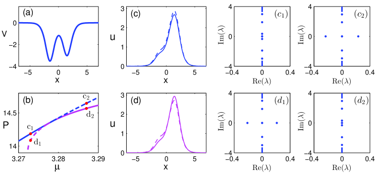
Figure 3: Stability switching at a transcritical bifurcation in Example (4.1). (a) The asymmetric double-well potential (4.2); (b) the power diagram; (c) profiles of solitary waves at locations $c_{1}$ (solid) and $c_{2}$ (dashed) of the upper power curve in (b); (d) profiles of solitary waves at locations $d_{1}$ (dashed) and $d_{2}$ (solid) of the lower power curve in (b). ($c_{1},c_{2},d_{1},d_{2}$) stability spectra for solitary waves at locations of the same letters on the power diagram (b).

5 Summary and discussion

In summary, linear stability of solitary waves near transcritical bifurcations was analyzed for the GNLS equations (2.1) with arbitrary forms of nonlinearity and external potentials in arbitrary spatial dimensions. It was shown that both solution branches undergo stability switching at the transcritical bifurcation point. In addition, the two solution branches have opposite stability. Analytical formulae for the unstable eigenvalues were also derived. These analytical stability results were compared with a numerical example and good agreement was obtained.

The above stability properties closely resemble those in finite-dimensional dynamical systems, where it is well known that the stability of fixed-point branches near a transcritical bifurcation point exhibits the same behaviors as above [17]. However, this happy resemblance, which we proved in this paper, should not be taken for granted. Indeed, it has been shown that for saddle-node and pitchfork bifurcations, stability properties in the GNLS equations differ significantly from those in finite-dimensional dynamical systems [9, 10, 18]. For instance, at a saddle-node bifurcation point, there is no stability switching in the GNLS equations (2.1) [9, 10], but any dynamical-system textbook would say that such stability switching takes place [17]. Thus it may be more appropriate to view this similar stability on transcritical bifurcations in the GNLS equations and finite-dimensional dynamical systems as a happy surprise rather than a trivial expectation.

Another approach to qualitatively study the linear stability of nonlinear waves in Hamiltonian systems is the Hamiltonian-Krein index theory [22, 23, 24, 25, 26]. In this approach, the number of unstable eigenvalues in the linear-stability operator ${\cal L}$ is related to the number of positive eigenvalues in operators $L_{0}$ and $L_{1}$ under appropriate conditions. Near a transcritical bifurcation point $\mu=\mu_{0}$, we can show that the zero eigenvalue in $L_{10}$ bifurcates out as

$$\Lambda_{\pm}(\mu)\to\frac{\pm\sqrt{\Delta}}{\langle\psi,\psi\rangle}\,(\mu-\mu_{0}),\qquad\mu\to\mu_{0},$$

where $\Lambda_{\pm}(\mu)$ is the eigenvalue of $L_{1}$ on the $u^{\pm}(\mathbf{x};\mu)$ solution branch. Using this formula, the qualitative stability results in Theorem 3 can be reproduced by the index theory (as was done in [18] for pitchfork bifurcations). However, this index-theory approach requires more restrictive conditions on the spectra of $L_{0}$ and $L_{1}$ operators [22, 25, 18], and it cannot yield quantitative linear-stability eigenvalue formula (2.15) either.

It should be recognized that transcritical bifurcations in the GNLS equations (2.1) occur less frequently than saddle-node or pitchfork bifurcations. Indeed, in the example (4.1), if the seventh-power coefficient $\kappa$ is not equal to that special value $\kappa_{c}$, this transcritical bifurcation would either turn into a pair of saddle-node bifurcations or disappear, depending on whether $\kappa$ is less than $\kappa_{c}$ or greater than $\kappa_{c}$. Due to this less frequent occurrence, one might wonder how useful the stability results in this paper are. To address this concern, it is helpful to view a transcritical bifurcation as the limit when two saddle-node bifurcations coalesce with each other (such as when $\kappa\to\kappa_{c}^{-}$ in the example (4.1)). In this connection, the stability results obtained in this paper for transcritical bifurcations can also be used to help determine stability properties of nearby saddle-node solution branches. Thus the stability results in this article can be useful beyond transcritical bifurcations.

References

- [1] O
- [2] Y. S. Kivshar and G. P. Agrawal, Optical Solitons: From Fibers to Photonic Crystals (Academic Press, San Diego, 2003).
- [3] J. Yang, Nonlinear Waves in Integrable and Nonintegrable Systems (SIAM, Philadelphia, 2010).
- [4] L.P. Pitaevskii and S. Stringari, Bose-Einstein Condensation (Oxford University Press, Oxford, 2003).
- [5] G. Herring, P.G. Kevrekidis, R. Carretero-González, B.A. Malomed, D.J. Frantzeskakis, and A.R. Bishop, “Trapped bright matter-wave solitons in the presence of localized inhomogeneities”, Phys. Lett. A 345, 144–153 (2005).
- [6] T. Kapitula, P. G. Kevrekidis, and Z. Chen, “Three is a crowd: Solitary waves in photorefractive media with three potential wells”, SIAM J. Appl. Dyn. Syst. 5, 598- 633 (2006).
- [7] C. Wang, P.G. Kevrekidis, N. Whitaker, D.J. Frantzeskakis, S. Middelkamp, and P. Schmelcher, “Collisionally inhomogeneous Bose-Einstein condensates in double-well potentials”, Physica D 238, 1362–1371 (2009).
- [8] T. R. Akylas, G. Hwang, and J. Yang, “From nonlocal gap solitary waves to bound states in periodic media”, Proc. Roy. Soc. A 468, 116–135 (2012).
- [9] J. Yang, “No stability swtching at saddle-node bifurcations of solitary waves in generalized nonlinear Schrödinger equations”, Phys. Rev. E 85, 037602 (2012).
- [10] J. Yang, “Conditions and stability analysis for saddle-node bifurcations of solitary waves in generalized nonlinear Schrödinger equations”, chapter in book Spontaneous Symmetry Breaking, Self-Trapping, and Josephson Oscillations in Nonlinear Systems, B.A. Malomed, ed. (Springer, Berlin, 2012).
- [11] M. Matuszewski, B.A. Malomed, and M. Trippenbach, “Spontaneous symmetry breaking of solitons trapped in a double-channel potential”, Phys. Rev. A 75, 063621 (2007).
- [12] E.W. Kirr, P.G. Kevrekidis, E. Shlizerman, and M.I. Weinstein, “Symmetry-breaking bifurcation in nonlinear Schrödinger/Gross- Pitaevskii equations,” SIAM J. Math. Anal. 40, 56 -604 (2008).
- [13] A. Sacchetti, “Universal critical power for nonlinear Schrodinger equations with symmetric double well potential,” Phys. Rev. Lett. 103, 194101 (2009).
- [14] C. Wang, G. Theocharis, P.G. Kevrekidis, N. Whitaker, K.J.H. Law, D.J. Frantzeskakis, and B.A. Malomed, “Two-dimensional paradigm for symmetry breaking: the nonlinear Schrödinger equation with a four-well potential,” Phys. Rev. E 80, 046611 (2009).
- [15] E.W. Kirr, P.G. Kevrekidis, and D.E. Pelinovsky, “Symmetry-breaking bifurcation in the nonlinear Schrodinger equation with symmetric potentials”, Commun. Math. Phys. 308, 795 -844 (2011).
- [16] J. Yang, “Classification of solitary wave bifurcations in generalized nonlinear Schrödinger equations”, Stud. Appl. Math. 129, 133–162 (2012).
- [17] J. Guckenheimer and P. Holmes, Nonlinear Oscillations, Dynamical Systems, and Bifurcations of Vector Fields (Springer-Verlag, New York 1990).
- [18] J. Yang, “Stability analysis for pitchfork bifurcations of solitary waves in generalized nonlinear Schr odinger equations”, to appear in Physica D (2012).
- [19] Y. V. Kartashov, B. A. Malomed, and L. Torner, “Solitons in nonlinear lattices”, Rev. Mod. Phys. 83, 247–306 (2011).
- [20] G. Hwang, T.R. Akylas and J. Yang, “Solitary waves and their linear stability in nonlinear lattices”, Stud. Appl. Math. 128, 275 -299 (2012).
- [21] M. Struwe, Variational Methods: Applications to Nonlinear Partial Differential Equations and Hamiltonian Systems (3rd ed.), Springer, Berlin, 2000. [Specifically the paragraph just below Theorem B.4 on page 246.]
- [22] T. Kapitula, P. Kevrekidis, and B. Sandstede, “Counting eigenvalues via the Krein signature in infinite-dimensional Hamiltonian systems,” Physica D 195, 263 -282 (2004).
- [23] T. Kapitula, P. Kevrekidis, and B. Sandstede, “Addendum: Counting eigenvalues via the Krein signature in infinitedimensional Hamiltonian systems,” Physica D 201, 199 -201 (2005).
- [24] D.E. Pelinovsky, “Inertia law for spectral stability of solitary waves in coupled nonlinear Schrödinger equations,” Proc. R. Soc. A 461, 783- 812 (2005).
- [25] M. Chugunova and D.E. Pelinovsky, “Count of eigenvalues in the generalized eigenvalue problem,” J. Math. Phys. 51, 052901 (2010).
- [26] T. Kapitula and K. Promislow, “Stability indices for constrained self-adjoint operators,” Proc. Amer. Math. Soc. 140, 865 -880 (2012).