Statefinder Analysis of f(T) Cosmology

Abstract

Abstract: In this paper, we intend to evaluate and analyze the statefinder parameters in $f(T)$ cosmology. Friedmann equation in $f(T)$ model is taken, and the statefinder parameters $\{r,s\}$ are calculated. We consider a model of $f(T)$ which contains a constant, linear and non-linear form of torsion. We plot $r$ and $s$ in order to characterize this model in the $\{r,s\}$ plane. We found that our model $f(T)=2C_{1}\sqrt{-T}+\alpha T+C_{2},$ predicts the decay of dark energy in the far future while its special case namely teleparallel gravity predicts that dark energy will overcome over all the energy content of the Universe.

I Introduction

The incompatibility of General Relativity (GR) as a complete theory of gravity came to light when the recent cosmological observations from Ia supernovae, CMBR via WMAP, galaxy redshift surveys via SDSS and and galactic X-ray indicated that the observable Universe enters into an epoch of accelerated expansion c1 ; c2 ; c3 ; c4 . In the quest of finding a suitable model for Universe, cosmologists started to investigate the root cause that is responsible for this expansion. Existence of a mysterious negative pressure component which violates the strong energy condition i.e. $\rho+3p<0$ is proposed as one of the major alternatives responsible for the recent cosmic acceleration. Because of its invisible nature this energy component is aptly termed as dark energy (DE) Riess1 (also see a recent review on DE bamba1 ). Quite surprisingly, observations show that about 70 percent of the Universe is filled by this unknown ingredient and in addition that about 25 percent of this is composed by dark matter (DM).

The simplest model for the accelerating universe is the Universe associated with a tiny cosmological constant $\Lambda$ c7 . But it was soon found that the model suffered from fine tuning and cosmic coincidence problems. So the search for a better model continued. With the passage of time, various models of DE were proposed and subsequently developed. Some of them are quintessence scalar fields quint , Chaplygin gas chaplygin , phantom energy field phant , f-essence f and interacting dark energy models obs ; cr ; pr . As so many cosmological DE models started appearing in the scene gradually, it became an utmost necessity to devise a method that will be able to either qualitatively or quantitatively differentiate between the various DE models. Hence in order to bring about this discrimination between the various contenders, Sahni et al Sahni1 proposed a new geometrical diagnostic named the statefinder pair $\left\{r,s\right\}$. Clear differences for the evolutionary trajectories in the $r-s$ plane have been found for different dark energy models in jamil . The statefinder parameters are defined as follows,

$$r\equiv\frac{\stackrel{{\scriptstyle...}}{{a}}}{aH^{3}}~{}~{}~{}~{}~{}~{}~{}~{}~{}~{}s\equiv\frac{r-1}{3\left(q-\frac{1}{2}\right)},$$ (1)

where $a$ is the scale factor of the Universe, $H$ is the Hubble parameter, a dot denotes differentiation with respect to the cosmic time $t$ and $q$ is the deceleration parameter given by,

$$q=-\frac{\dddot{a}}{aH^{2}}.$$ (2)

It is found that for the $\Lambda$CDM model, $r=1$ and $s=0$.

In order to bring about the discrimination between various DE models the trajectories in the $r-s$ plane for these models are generated. The distances of the contrasting $r-s$ trajectories of these models from $(0,1)$ point is computed. These computed distances, as expected, vary significantly from model to model, thus giving us an extremely useful tool to differentiate between various cosmological DE models. Thus the difference in the trajectory from the standard $\Lambda$CDM model produces the required discrimination and characterizes the given model up to a great extent pano .

A section of cosmologists concentrated on the left hand side of the Einstein’s equation ($G_{\mu\nu}=8\pi GT_{\mu\nu}$) rather than the right hand side in order find an effective modification that will admit the recent cosmic acceleration in its framework. They ended up modifying the Einstein gravity and giving birth to various modified gravity theories. This alternative method along with the concept of DE have gained enormous popularity in the cosmological society since it passes several solar system and astrophysical tests successfully sergei2 . It is found that both the methods (DE and modified gravity models) can successfully account for the recent cosmic acceleration independently. In the context of modified gravity theory it is worth stating that Loop quantum gravity lqc , extra dimensional braneworlds brane , $f(R)$ fr , $f(T)$ ft ; miao ; miaoli ; sotirio are some of the popular modified gravity models.

An attempt to unify gravitation with electromagnetism gave birth to Teleparallelism (Einstein). But as the years passed by scientists lost interest in this concept of unification because of the conceptual and physical diversity of various physical theories. As a result, today teleparallelism stands just as a theory of gravity. Teleparallel gravity corresponds to a gauge theory for the translation group trans . Einstein introduced the crucial new idea of a tetrad field in this theory. Here the space-time is characterized by a curvature-free linear connection, called the Weitzenbock connection. Since the space-time is free from curvature, it is quite evident that the theory in its physical aspect is quite different from the Einstein gravity, whose main feature is curvature. In Teleparallelism, curvature is in fact substituted by torsion, another physical tool responsible for the dynamics of space-time. In the framework of general relativity (GR), curvature is used to geometrize space-time, thus successfully describing the gravitational interaction between particles. But in Teleparallelism, the role of gravitation is played by torsion not by geometrizing the interaction (unlike curvature), but by merely acting as a force. This implies that, in the teleparallel gravity, instead of geodesics, there are force equations, which are analogous to the Lorentz force equation of electrodynamics trans thus bridging the two theories upto certain extents.

The paper is organized as follows. In section II, the basic equations for the $f(T)$ model is discussed and the statefinder parameters are calculated. In section III, a model of $f(T)$ gravity is considered, and the statefinder parameters are evaluated. A detailed physical analysis is done in section IV. Finally we end with some concluding remarks in section V.

II $f(T)$ gravity and dynamical equations

$f(T)$ gravity developed as an alternative theory for GR, defined on the Weitzenbock manifold, working only with torsion with no curvature. A manifold is divided into two separate parts connected with each other. One part having a Riemannian structure with a definite metric described on it and another part having a non-Riemannian structure with torsion or non-metricity. The part having zero Riemannian tensor but having non zero torsion represents a Weitzenbock spacetime. If $f(T)=T$ , this theory reduces to teleparallel gravity hayashi ; hehl . It is seen that with linear $T$ , this model has many common features like GR and satisfies some standard tests of the GR in solar system hayashi . A general model of $f(T)$ was proposed only a few years back f(T) . This model has many important features. Birkhoff s theorem has already been studied in this gravity birkhoff . The authors in zheng investigated perturbation in $f(T)$ and found that the perturbation in $f(T)$ gravity grows slower than that in Einstein GR. Bamba et al bamba studied the evolution of equation of state parameter and phantom crossing in $f(T)$ model. Emergent Universes in chameleon $f(T)$ model is investigated in chat . Also it is found that the dark matter problem can be addressed and resolved in $f(T)$ gravity dm . In this paper we intend to perform a complete analysis of the statefinder parameters in various $f(T)$ models.

A suitable form of action for $f(T)$ gravity in Weitzenbock spacetime is f(T)

$$\mathcal{S}=\frac{1}{2\kappa^{2}}\int d^{4}xe\left(T+f(T)+\mathcal{L}_{m}\right).$$

Here $e=det(e^{i}_{\mu})=\sqrt{-g}$, $\kappa^{2}=8\pi G$ and $e^{i}_{\mu}$ is the tetrad (vierbein) basis. The dynamical quantity of the model is the vierbein $e^{i}_{\mu}$ and $L_{m}$ is the matter Lagrangian. The Friedmann equation in this form of the $f(T)$ model f(T) is given by,

$$H^{2}=\frac{1}{1+2f_{T}}\Big{(}\frac{\kappa^{2}}{3}\rho-\frac{f}{6}\Big{)},$$ (3)

where $\rho=\rho_{m}$, while $\rho_{m}$ represents the energy densities of matter. Here $f_{T}=\frac{df}{dT}$ and $f$ is a function of $T$.

Another FRW equation is

$$\dot{H}=-\frac{\kappa^{2}}{2}\Big{(}\frac{\rho+p}{1+f_{T}+2Tf_{TT}}\Big{)}.$$ (4)

Here $f_{TT}=\frac{d^{2}f}{dT^{2}}$. It is useful to rewrite the equations (3) and (4) in the following suitable form

$$H^{2} = \frac{\kappa^{2}}{3}\left(\rho_{m}+\rho_{T}\right),$$ (5)

$$\dot{H} = -\frac{\kappa^{2}}{2}\left(\rho_{m}+\rho_{T}+p_{T}\right),$$ (6)

where

$$\rho_{T} = \frac{1}{\kappa^{2}}\left(-\frac{f}{2}+Tf_{T}\right),$$ (7)

$$p_{T} = \frac{1}{\kappa^{2}}\left[\frac{f}{2}+\left(2\dot{H}-T\right)f_{T}+4T\dot{H}f_{TT}\right].$$ (8)

The dimensionless density parameters are defined by

$$\Omega_{m}+\Omega_{T}=1,\ \ \Omega_{m}=\frac{\kappa^{2}\rho_{m}}{3H^{2}},\ \ \Omega_{T}=\frac{\kappa^{2}\rho_{T}}{3H^{2}}.$$ (9)

Easily we can write the following expression for deceleration parameter $q$ and equation of state (EoS) parameter $w$,

$$q=\frac{1}{2}\left(1+3w\Omega_{T}\right),\ \ ~{}~{}~{}~{}w=\frac{p_{T}}{\rho_{T}}=-1+4\dot{H}\Phi,\ \ \Phi\equiv\frac{f_{T}+2Tf_{TT}}{-f+2Tf_{T}}.$$ (10)

Further, the evolutionary equation for $\Omega_{T}$ reads

$$\dot{\Omega}_{T}=3HT\left(\frac{f_{T}}{T}-\frac{f}{T^{2}}-2f_{TT}\right)\left(1+w\Omega_{T}\right).$$ (11)

The state finder parameter $r$ can also be written as

$$r=2q^{2}+q-\frac{\dot{q}}{H}.$$ (12)

Using equations (10) and (11) in (12) we obtain the statefinder parameters for $f(T)$ cosmology:

$$r = \frac{1}{2}\left[\Big{(}1+3\left(-1+4\dot{H}\Phi\right)\Omega_{T}\Big{)}^{2}+\Big{(}1+3\left(-1+4\dot{H}\Phi\right)\Omega_{T}\Big{)}\right]$$ (13)

$$-\frac{3}{2H}\Big{[}\dot{w}\Omega_{T}+3wH\left(1+w\Omega_{T}\right)\left(\frac{f_{T}}{T}-\frac{f}{T^{2}}-2f_{TT}\right)\Big{]},$$

$$s=\frac{2(r-1)}{9(-1+4\dot{H}\Phi)\Omega_{T}}.$$ (14)

where

$$\dot{w}=4\Big{(}\ddot{H}\Phi+\dot{H}\dot{T}\frac{d\Phi}{dT}\Big{)}.$$ (15)

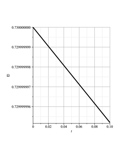
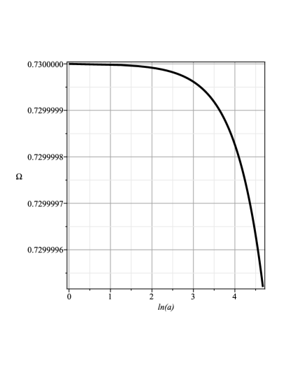
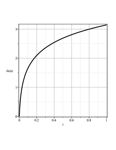
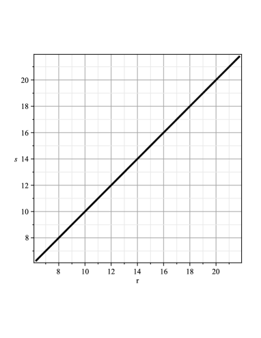
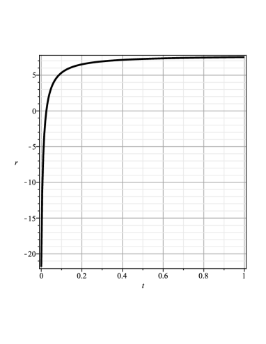
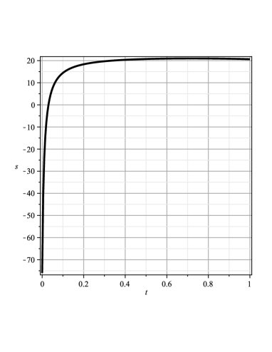
Figure 1: (Top Left) Cosmic energy density parameter $\Omega$ against time. (Top Right) Cosmic energy density parameter $\Omega$ against logarithmic scale factor. (Middle Left) Evolution of scale factor with time. (Middle Right) Statefinder parameters $\{r,s\}$ against each other. (Bottom Left) Parameter $r$ vs time. (Bottom Right) Parameter $s$ vs time. While plotting these figures, we assumed $\Omega_{0m}\simeq 0.2$, $C_{2}=0$, $\alpha=0.2$, $\Omega_{d0}\simeq 0.73$, $H_{0}\simeq 74$.

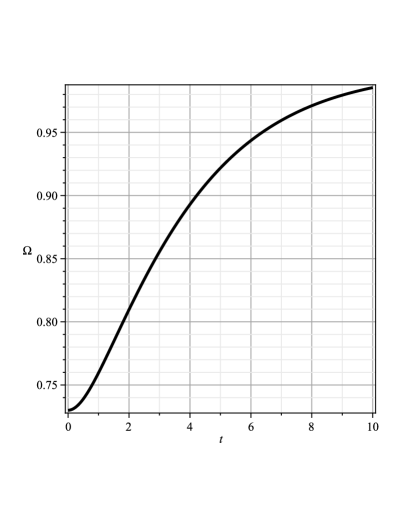
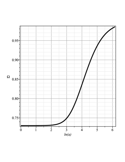
Figure 2: (Left) Cosmic energy density parameter $\Omega$ against time for teleparallel gravity. (Right) Cosmic energy density parameter $\Omega$ against logarithmic scale factor for teleparallel gravity. Here we put $C_{1}=0$ and $C_{2}=0.1$ and used the same initial conditions as Figure-1.

III Statefinder parameters for a particular $f(T)$

In order to avoid analytic and computation problems, we choose a suitable expression for $f(T)$ which contains a constant, linear and a non-linear form of torsion, specifically attractor

$$f(T)=2C_{1}\sqrt{-T}+\alpha T+C_{2},$$ (16)

where $\alpha$, $C_{1}$ and $C_{2}$ are arbitrary constants. Note that choosing $C_{1}=0$ in (16) leads to teleparallel gravity.

In this model the combination of the first and the third term corresponds to the EoS of the cosmological constant in the framework of $f(T)$ gravity mirza . In this way by shuffling various terms or by the introduction of new terms, cosmologists all over the world have succeeded in establishing different models. In fact many of them have been reconstructed from various dark energy models. The model in equation (16) that we are currently dealing with may have been inspired from the proposed model of Veneziano ghost kk .

As a matter of fact this model was preferentially chosen over other alternatives, purely because of its simplicity as far as numerical computation is concerned. Another advantage of this model is that the obtained results are easier to compare or differentiate from the corresponding results in GR. In order to facilitate this, the linear middle term is included in the model. In connection with this model, it is worth stating that Capozziello et al capo123 made an attempt to investigate the cosmography of $f(T)$ cosmology by using data from BAO, Supernovae Ia and WMAP. The analysis performed by Capozziello and his colleagues unveiled the fact that by choosing $C_{2}=0$,  $\alpha=\Omega_{m0}$ and $C_{1}=\sqrt{6}H_{0}\left(\Omega_{m0}-1\right)$, it is possible to estimate the parameters of our proposed $f(T)$ model as functions of Hubble parameter $H_{0}$, the cosmographic parameters and the value of matter density parameter.

Using this model we have the following expressions for the statefinder parameters,

$$r = \frac{1}{72\left(H\left(t\right)\right)^{5}}\left[144\,\left({\frac{d}{dt}}H\left(t\right)\right)^{2}H\left(t\right)\Omega_{{{\it m0}}}+144\,H\left(t\right){\Omega_{{{\it m0}}}}^{2}\left({\frac{d}{dt}}H\left(t\right)\right)^{2}+432\,\left(H\left(t\right)\right)^{3}{\Omega_{{{\it m0}}}}^{2}{\frac{d}{dt}}H\left(t\right)\right.$$ (17)

$$\left.+216\,\left(H\left(t\right)\right)^{3}\Omega_{{{\it m0}}}{\frac{d}{dt}}H\left(t\right)-72\,\left(H\left(t\right)\right)^{2}\left({\frac{d^{2}}{d{t}^{2}}}H\left(t\right)\right)\Omega_{{{\it m0}}}+72\,\left(H\left(t\right)\right)^{5}+324\,\left(H\left(t\right)\right)^{5}\Omega_{{{\it m0}}}\right.$$

$$\left.+324\,\left(H\left(t\right)\right)^{5}{\Omega_{{{\it m0}}}}^{2}\right],$$

$$s = \frac{1}{18\left(H\left(t\right)\right)^{3}\left(6\,\left(H\left(t\right)\right)^{2}+4\,{\frac{d}{dt}}H\left(t\right)\right)\,}\left[48\left({\frac{d}{dt}}H\left(t\right)\right)^{2}H\left(t\right)+48\,\left({\frac{d}{dt}}H\left(t\right)\right)^{2}H\left(t\right)\Omega_{{{\it m0}}}\right.$$ (18)

$$\left.+144\,\left(H\left(t\right)\right)^{3}\Omega_{{{\it m0}}}{\frac{d}{dt}}H\left(t\right)+72\,\left(H\left(t\right)\right)^{3}{\frac{d}{dt}}H\left(t\right)-24\,\left({\frac{d^{2}}{d{t}^{2}}}H\left(t\right)\right)\left(H\left(t\right)\right)^{2}+108\,\left(H\left(t\right)\right)^{5}\right.$$

$$\left.+108\,\left(H\left(t\right)\right)^{5}\Omega_{{{\it m0}}}\right],$$

where $\Omega_{{{\it m0}}}$ is the present dimensionless fractional matter density, such that $\Omega_{{{\it m0}}}=\frac{\rho_{{{\it m0}}}}{3H_{0}^{2}}$. Here $\rho_{{{\it m0}}}$ is the present matter density and $H_{0}$ is the present Hubble parameter. In accordance with the current observational data the value of $\Omega_{{{\it m0}}}$ is almost equal to $0.27$. It is interesting to note that for present time the $\{r,s\}$ parameters take the form

$$r = 1+4.5\Omega_{\it m0}(1+\Omega_{\it m0}),$$ (19)

$$s = 1+\Omega_{\it m0}.$$ (20)

IV Numerical results and physical aspects

In this section, we will solve the time evolutionary equations (6) and (11) by numerical algorithms. We adopt the initial conditions as $\Omega_{0m}=0.2$, $C_{2}=0$, $\alpha=0.2$, $\Omega_{d0}=0.73$, $H_{0}=74$. It is observed that these are regular solutions and the generic form of the solutions is independent from the initial conditions imposed on the functions. In figure-1, the top left and right figures represent the evolution of density parameter $\Omega_{T}$ against time and logarithmic scale factor. In either figures, it is easily seen the energy density parameter decreases and vanish in the far future. This shows that if dark energy is represented by the torsion of space, it will decay in far future. Moreover the middle left figure in the same panel shows that the slope of logarithmic scale factor is concave downwards, i.e. the model predicts deceleration on account of decaying dark energy. Middle right figure shows the trajectory of the chosen $f(T)$ in the $\{r,s\}$ plane. The bottom left and right figures give the evolutionary trajectories of $r$ and $s$ independently. It is interesting to note that trajectories of both parameters are essentially identical except the rescaling of the vertical coordinate. In figure-2, we plot figures for the teleparallel gravity by choosing $C_{1}=0,$ and adopting the same initial conditions. Contrary to the previous case, the teleparallel gravity predicts the increase in the dark energy density i.e. $\Omega_{T}\rightarrow 1.$ In other words, the dark energy component due to torsion will overcome on all the remaining energy content of the Universe.

V Conclusion

We have performed a complete analysis of statefinder parameters in $f(T)$ gravity, which is a mere modification of the teleparallel gravity once proposed by Einstein. We considered a model containing linear and non-linear terms of $T$) have been considered and a complete diagnosis of the statefinder parameters have been carried out. Plots have been generated for the statefinder parameters $r$ and $s$ with respect to the Hubble parameter $H$, for different values of model parameters. This gives us a clear notion about the nature of the modified gravity theory $f(T)$ and its governing dynamics. Specifically we found that our model $f(T)=2C_{1}\sqrt{-T}+\alpha T+C_{2},$ predicts of decay of dark energy in the far future while its special case namely teleparallel gravity predicts that dark energy will overcome over all the energy content of the Universe. We hope that by comparing the statefinder analysis illustrated in this work with the future observational data, $f(T)$ models can be distinguished from the $\Lambda$CDM model.

Acknowledgments

We would like to thank anonymous referee for giving useful comments to improve this paper.

References

- (1) S. Perlmutter et al., Astrophys. J. 517, 565 (1999); D. N. Spergel et al. Astron. J. Suppl 148, 175 (2003).
- (2) C.L. Bennett et al., Astrophys. J. Suppl. 148, 1 (2003).
- (3) M. Tegmark et al., Phys. Rev. D 69, 103501 (2004).
- (4) S.W. Allen et al., Mon. Not. Roy. Astron. Soc. 353, 457 (2004).
- (5) A.G. Riess et al., Astron. J. 116, 1009 (1998).
- (6) K. Bamba, S. Capozziello, S. Nojiri, S.D. Odintsov, Astrophysics and Space Science, DOI: 10.1007/s10509-012-1181-8 [arXiv:1205.3421v3 [gr-qc]]
- (7) V. Sahni, A. Starobinsky, Int. J. Mod. Phy. D 9, 373 (2000); P.J. Peebles, B. Ratra, Rev. Mod. Phys. 75, 559 (2003);
- (8) B. Ratra, P.J.E. Peebles, Phys. Rev. D 37, 3406 (1988); C. Wetterich, Nucl. Phys. B 302, 668 (1988); A. R. Liddle, R.J. Scherrer, Phys. Rev. D 59, 023509 (1999).
- (9) A. Kamenshchik, U. Moschella, V. Pasquier, Phys. Lett. B 511, 265 (2001); M. Jamil, M.A. Rashid, Eur. Phys. J. C 58, 111 (2008); M. Jamil, M.A. Rashid, Eur. Phys. J. C 60, 141 (2009); M. Jamil, Int. J. Theor. Phys. 49, 62 (2010); M. Jamil, Int. J. Theor. Phys. 49, 144 (2010); M.U. Farooq, M.A. Rashid, M. Jamil, Int. J. Theor. Phys. 49, 2334 (2010).
- (10) R. R. Caldwell, Phys. Lett. B 545, 23 (2002); R.R. Caldwell, M. Kamionkowski, N.N. Weinberg, Phys. Rev. Lett. 91, 071301 (2003); M. Jamil, S. Ali, D. Momeni, R. Myrzakulov, Eur. Phys. J. C 72, 1998 (2012); M. Jamil, D. Momeni, M. Raza, R. Myrzakulov, Eur. Phys. J. C 72, 1999 (2012).
- (11) M. Jamil, Y. Myrzakulov, O. Razina, R. Myrzakulov, Astrophys. Space Sci. 336, 315 (2011); M. Jamil, D. Momeni, N. S. Serikbayev, R. Myrzakulov, Astrophys. Space Sci. 339, 37 (2012).
- (12) H. Wei, S. N. Zhang, Phys. Lett. B 654, 139 (2007); M-L Tong, Y Zhang, Z-W Fu, Class. Quant. Grav. 28, 055006 (2011); Y-H Li, J-Z Ma, J-L. Cui, Z. Wang, X. Zhang, Sci. China Phys. Mech. Astron. 54, 1367 (2011); H. Wei, Phys. Lett. B 691, 173 (2010); S. M. R. Micheletti, JCAP 1005, 009 (2010); C. Feng, B. Wang, E. Abdalla, R-K. Su, Phys. Lett. B 665, 111 (2008); L. Amendola, C. Quercellini, D. T-Valentini, A. Pasqui, Astrophys.J. 583, L53 (2003).
- (13) G. Olivares, F. A-Barandela, D. Pavon, Phys. Rev. D 77, 063513 (2008).
- (14) M Jamil, A Sheykhi, M. U Farooq, Int. J. Mod. Phys. D 19, 1831 (2010); K. Karami, A. Sheykhi, M. Jamil, Z. Azarmi, M. M. Soltanzadeh, Gen. Relativ. Grav. 43, 27 (2011); M. Jamil, E. N. Saridakis, JCAP 1007, 028 (2010); P. Rudra, U. Debnath, R. Biswas, Astrophys Space Sci (2012) 339:53 64; R. Chowdhury, P. Rudra, [arXiv:1204.3531 [gr-qc]]; M. Jamil, M.A. Rashid, Eur. Phys. J. C 56, 429 (2008); M. Jamil, F. Rahaman, Eur. Phys. J. C 64, 97 (2009).
- (15) V. Sahni, T.D. Saini, A.A. Starobinsky, U. Alam, JETP Lett. 77, 201 (2003).
- (16) M.R. Setare, M. Jamil, Gen. Relativ. Gravit. 43, 293 (2011); M. Jamil, M. Raza, U. Debnath, Astrophys. Space Sci. 337, 799 (2012); S. Chakraborty, U. Debnath, M. Jamil, Canadian J. Phys. 90, 365 (2012); M. Jamil, I. Hussain, D. Momeni, Eur. Phys. J. Plus 126, 80 (2011); U. Debnath, M. Jamil, Astrophys. Space Sci. 335, 545 (2011); M. Jamil, Int. J. Theor. Phys. 49, 2829 (2010); M. Jamil, U. Debnath, Int. J. Theor. Phys. 50, 1602 (2011).
- (17) G. Panotopoulos, Nucl.Phys.B. 796, 66-76 (2008)
- (18) S. Nojiri, S. D. Odintsov, Phys. Rept. 505, 59 (2011); S. Capozziello, M. De Laurentis, arXiv:1108.6266v2 [gr-qc]; T. Clifton, P. G. Ferreira, A. Padilla, C. Skordis, arXiv:1106.2476v2 [astro-ph.CO]
- (19) C. Rovelli, liv. Rev. Rel.1, 1 (1998); A. Ashtekar, J. Lewandowski, Class. Quantum. Grav. 21, R53 (2004); M. Jamil, D. Momeni, M.A. Rashid, Eur. Phys. J. C 71, 1711 (2011); M. Jamil, U. Debnath, Astrophys. Space Sci. 333, 3 (2011); D. Dwivedee, B. Nayak, M. Jamil, L.P. Singh, arXiv:1110.6350v2 [gr-qc].
- (20) Maartens, R., Phys. Rev. D 62, 084023 (2000); R. Maartens, Living Rev. Relativity 7, 7 (2004).
- (21) R. Kerner, Gen. Relativ. Gravit. 14, 453 (1982); G. Allemandi, A. Borowiec, M. Francaviglia, Phys. Rev. D 70, 103503 (2004); S.M. Carroll, A.D. Felice, V.Duvvuri, D.A. Easson, M. Trodden, M.S. Turner, Phys. Rev. D 71, 063513 (2005); T.P. Sotiriou, V. Faraoni, gr-qc/0805.1726.
- (22) K. K. Yerzhanov et al, arXiv:1006.3879v1 [gr-qc]; R. Myrzakulov (2010), arXiv:1006.1120v1 [gr-qc]; E. V. Linder, Phys. Rev. D 81 127301 (2010).
- (23) M. Li, R-X Miao, Y-G Miao, JHEP 1107, 108 (2011).
- (24) R. Miao, M. Li, Y. Miao, JCAP 11, 033 (2011).
- (25) B. Li, T. P. Sotiriou, J. D. Barrow, Phys. Rev. D 83, 064035 (2011).
- (26) V. C. de Andrade, J. G. Pereira, Phys. Rev D 56, 4689 (1997); F. W. Hehl, J. D. McCrea, E. W. Mielke, Y. Ne eman, Phys. Rep. 258, 1 (1995).
- (27) K. Hayashi, T. Shirafuji, Phys. Rev. D 19, 3524 (1979); K. Hayashi, T. Shirafuji, Phys. Rev. D 24, 3312 (1981).
- (28) F. Hehl, P. von der Heyde, G. Kerlick, Rev. Mod. Phys. 48, 393 (1976).
- (29) R.Ferraro, F.Fiorini, Phys. Rev. D 75, 084031 (2007); R. Ferraro, F. Fiorini, Phys. Rev. D 78, 124019 (2008).
- (30) X. Meng, Y. Wang, Eur. Phys. J. C 71 (2011) 1755.
- (31) R. Zheng, Q-G. Huang, JCAP 1103, 002 (2011).
- (32) K. Bamba, C-Q Geng, C-C Lee, L-W Luo, JCAP 1101, 021 (2011).
- (33) S. Chattopadhyay, U. Debnath, Int. J. Mod. Phys. D 20, 1135 (2011).
- (34) M. Jamil, D. Momeni, R. Myrzakulov, Eur. Phys. J. C 72, 2122 (2012).
- (35) M. Jamil, D. Momeni, R. Myrzakulov, Eur. Phys. J. C 72, 1959 (2012).
- (36) R. Myrzakulov, Eur. Phys. J. C 71, 1752 (2011).
- (37) K. Karami, A. Abdolmaleki, arXiv:1202.2278.
- (38) S. Capozziello, V.F. Cardone, H. Farajollahi, A. Ravanpak, Phys. Rev. D 84, 043527 (2011).