Cosmology in $f(R)$ exponential gravity

Abstract

Using an approach that treats the Ricci scalar itself as a degree of freedom, we analyze the cosmological evolution within an $f(R)$ model that has been proposed recently (exponential gravity) and that can be viable for explaining the accelerated expansion and other features of the Universe. This approach differs from the usual scalar–tensor method and, among other things, it spares us from dealing with unnecessary discussions about frames. It also leads to a simple system of equations which is particularly suited for a numerical analysis.

1 Introduction

Since the discovery of the accelerated expansion of the Universe from the observations of supernovae Ia [17, 18, 1] and its interpretation using the $\Lambda$CDM model of standard cosmology, a large amount of investigations have been devoted to explain the same phenomenon but using dark energy substances different from the cosmological constant $\Lambda$. One can rank the dark energy models from the most “conservative” to the most “radical” ones. Among the former we can mention those which do not introduce new fields or modifications to general relativity but which consider that inhomogeneities in the Universe could be enough to account for the observations [15]. There are also the models that introduce new fields and perfect fluids with exotic equations of state within the framework of general relativity (GR) in order to avoid the “problems” associated with $\Lambda$ [19, 5, 14, 3]. For instance, quintessence, $k$–essence, and Chaplygin gas are some of the most popular models of this kind. The most radical attempts to explain the accelerated expansion are perhaps those which propose to modify GR while keeping the hypothesis of homogeneity and isotropy as a first approximation. Many alternate theories of gravity have been proposed to explain this phenomenon as well as those related with the dark matter (e.g. rotation curves of galaxies). The modified $f(R)$ metric gravity is just one of such theories and maybe the most analyzed one in the last ten years, where the geometry takes care of mimicking the dark energy. This alternative is certainly radical since GR has been thoroughly tested for almost one hundred years and it has not only supported all the tests but in addition most of its predictions have been confirmed as well. Thus, the challenge of modified gravity is both to be consistent with GR tests and also to explain the phenomena they were called for. This is a no trivial task and many $f(R)$ models have failed in the attempt. The story concerning dark substances does not end with the accelerated expansion. The measurements of the angular distribution of cosmic background radiation anisotropies in the sky can also be explained by the $\Lambda$CDM model, and therefore, the task for the alternative models, theories or dark energy substances is even more demanding.

As we mentioned, $f(R)$ theories have been studied in detail in a recent past and it is out of the scope of the present article to discuss all the properties, problems and features associated with some of the specific models proposed before (see Refs.  [16, 10, 20, 4, 6] for a review).

Our aim is to report the results of a potentially viable candidate, termed exponential gravity, as a model for the accelerated expansion, but using an approach that has been proposed recently by us [11] and which avoids the identification with the scalar–tensor theories. The reason to follow this “unorthodox” method is because in some cases the scalar–tensor (ST) method can lead to ill-defined potentials, and moreover because we want to circumvent any possible discussion concerning the use of frames (Einstein vs Jordan). Debates of this sort plague the subject, some of which have only led to create confusion instead of shedding light.

With our technique we propose to treat the Ricci scalar itself as a degree of freedom, instead of using $\phi=f_{R}$ as in the ST method (hereafter a subindex $R$ indicates $\partial/\partial_{R}$). Our approach also spare us of inverting all the quantities depending on $R$ for treating them as functions of $\phi$. Moreover, we have found that in several specific applications the field equations can be recasted in a rather friendly way that allows us to treat them numerically or even analytically [12, 11]. In the next section we present our method and apply it to the Friedmann-Roberson-Walker (FRW) spacetime within the scope of analyzing the cosmological evolution using the exponential gravity model. The analysis of other viable $f(R)$ models using the current approach can be seen in [11] and in references therein using other techniques.

2 $f(R)$ theories, the Ricci scalar approach

The action in $f(R)$ gravity is given by:

$$S[g_{ab},{\mbox{\boldmath{$\psi$}}}]=\!\!\int\!\!\frac{f(R)}{2\kappa}\sqrt{-g}\>d^{4}x+S_{\rm matt}[g_{ab},{\mbox{\boldmath{$\psi$}}}]\;,$$ (1)

where $\kappa\equiv 8\pi G_{0}$ (we use units where $c=1$), $f(R)$ is a sufficiently differentiable but otherwise a priori arbitrary function of the Ricci scalar $R$, and $\psi$ represents schematically the matter fields. The field equation obtained from Eq. (1) is:

$$f_{R}R_{ab}-\frac{1}{2}fg_{ab}-\left(\nabla_{a}\nabla_{b}-g_{ab}\Box\right)f_{R}=\kappa T_{ab}\,\,,$$ (2)

where $f_{R}$ indicates $\partial_{R}f$, $\Box=g^{ab}\nabla_{a}\nabla_{b}$ is the covariant D’Alambertian and $T_{ab}$ is the energy-momentum tensor (EMT) of matter associated with the $\psi$ fields. From this equation it is straightforward to obtain the following equation and its trace [12, 11]

$$G_{ab}=\frac{1}{f_{R}}\Bigl{[}f_{RR}\nabla_{a}\nabla_{b}R+f_{RRR}(\nabla_{a}R)(\nabla_{b}R)-\frac{g_{ab}}{6}\Big{(}Rf_{R}+f+2\kappa T\Big{)}+\kappa T_{ab}\Bigl{]}\;,$$ (3)

$$\Box R=\frac{1}{3f_{RR}}\Big{[}\kappa T-3f_{RRR}(\nabla R)^{2}+2f-Rf_{R}\Big{]}\;,$$ (4)

where $(\nabla R)^{2}:=g^{ab}(\nabla_{a}R)(\nabla_{b}R)$ and $T:=T^{a}_{\,\,a}$.

The idea is then to solve simultaneously Eqs. (3) and (4) for the metric $g_{ab}$ and $R$ as a system of coupled partial differential equations.

It is important to mention that the field equations imply that the EMT of matter alone is conserved, i.e., it satisfies $\nabla_{a}T^{ab}=0$.

In this contribution we shall focus on the model $f(R)=R_{*}[{\tilde{R}}-\lambda(1-e^{-{\tilde{R}}})]$, referred to as exponential gravity, where ${\tilde{R}}=R/R_{*}$, $\lambda$ is a positive dimensionless constant and $R_{*}>0$ is also a constant that fixes the built-in scale and which is of the order of the current Hubble parameter $H_{0}^{2}$. This kind of exponential models have been analyzed in the past by several authors using a different technique [8, 13, 21, 2, 9, 7]. Other variants of this model have also been analyzed [22]. The scalar $f_{R}=1-\lambda e^{-{\tilde{R}}}$ is positive provided $R>R_{*}{\rm ln}\lambda$ and this condition ensures $G_{\rm eff}:=G_{0}/f_{R}>0$. This latter is always satisfied in the cosmological solutions given below. The possible de Sitter points correspond to trivial solutions $R=R_{1}=const.$ of Eq. (4) in vacuum ($T=0$) and give rise to an effective cosmological constant $\Lambda_{\rm eff}=R_{1}/4$ in Eq. (3) ($G_{ab}=-g_{ab}\Lambda_{\rm eff}$ in vacuum). Here $R_{1}>0$ is a critical point of the “potential” $V(R)$ such that $V_{R}(R_{1})=0$ with $V_{R}:=(2f-Rf_{R})/3=R_{*}[{\tilde{R}}(1+\lambda e^{-{\tilde{R}}})-2\lambda(1-e^{-{\tilde{R}}})]/3$, and $V_{RR}=1-\lambda(1+{\tilde{R}})e^{-{\tilde{R}}}$. The “potential” is given by $V(R)=R_{*}^{2}[{\tilde{R}}({\tilde{R}}-4\lambda)-2\lambda({\tilde{R}}+3)e^{-{\tilde{R}}})]/6$. For $0<\lambda\leq 1$ one can easily see that $V(R)$ has just one critical point at $R=0$ which is not a de Sitter point as in this case $\Lambda_{\rm eff}\equiv 0$. The point is a global minimum (c.f. $V_{RR}(0)=1-\lambda$). For $\lambda>1$ there is a local maximum at $R=0$ and a global minimum at $R=R_{1}>0$ which corresponds to the actual de Sitter point that the cosmological solution reaches asymptotically in the future. There is also a local minimum at $R=R_{2}<0$, but it is an anti de Sitter point which is never reached as the cosmological solutions take place only in the domain $R>0$. The potential $V(R)$ is depicted in Figure 1 (right panel) where one can appreciate the critical points just described. In the high curvature regime ${\tilde{R}}\gg 1$, we have $f(R)\approx R-\lambda R_{*}$, and thus the model acquires an effective cosmological constant $\Lambda_{\rm eff}^{\infty}:=\lambda R_{*}/2$ (c.f. left panel of Fig. 1). From the figure we see that for $\lambda$ sufficiently high, the de Sitter point verifies ${\tilde{R}}_{1}\gg 1$, and thus $R_{1}\approx 2\lambda R_{*}$ as it turns out from $V_{R}(R_{1})=0$. Therefore $\Lambda_{\rm eff}\approx\Lambda_{\rm eff}^{\infty}$. Finally, we stress that $f_{RR}=\lambda e^{-{\tilde{R}}}/R_{*}>0$ which ensures that no singularities are found in the equations due to this scalar and moreover it guarantees that given $V_{RR}(R_{1})>0$ the effective mass $m^{2}:=V_{RR}/f_{RR}=(f_{R}-Rf_{RR})/(3f_{RR})|_{R_{1}}$ of the scalar mode is positive.

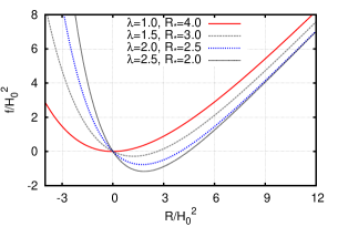
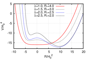
Figure 1: (color online) $f(R)$ exponential gravity (left panel) and the potential $V(R)$ (right panel) for several values of $\lambda$.

3 Cosmology in $f(R)$

We assume the spatially flat FRW metric given by:

$$ds^{2}=-dt^{2}+a^{2}(t)\left[dr^{2}+r^{2}\left(d\theta^{2}+\sin^{2}\theta d\varphi^{2}\right)\right]\,\,\,.$$ (5)

From Eqs. (3) and  (4) we have,

$$\ddot{R}=-3H\dot{R}-\frac{1}{3f_{RR}}\left[3f_{RRR}\dot{R}^{2}+2f-f_{R}R+\kappa T\right]\,\,\,,$$ (6)

$$H^{2}=\frac{\kappa}{3}\left(\rule{0.0pt}{8.5359pt}\rho+\rho_{X}\right)\,\,\,,$$ (7)

$$\dot{H}=-H^{2}-\frac{\kappa}{6}\left\{\rule{0.0pt}{11.38092pt}\rho+\rho_{X}+3\left(p_{\rm rad}+p_{X}\right)\right\}\,\,\,.$$ (8)

where a dot stands for $d/dt$ and $H=\dot{a}/a$, is the Hubble expansion. In the above equations we have included the energy density $\rho$ associated with matter (baryons, dark matter and radiation) as well as the GDE density $\rho_{X}$ and pressure $p_{X}$ given respectively by [11]

$$\rho_{X}=\frac{1}{\kappa f_{R}}\left\{\rule{0.0pt}{14.22636pt}\frac{1}{2}\left(f_{R}R-f\right)-3f_{RR}H\dot{R}+\kappa\rho\left(1-f_{R}\right)\right\},$$ (9)

$$p_{X}=-\frac{1}{3\kappa f_{R}}\left\{\frac{1}{2}\left(f_{R}R+f\right)+3f_{RR}H\dot{R}-\kappa\left(\rho-3p_{\rm rad}f_{R}\right)\right\}\,\,\,.$$ (10)

Another differential equation that can be used to solve for $H$ instead of Eq. (8) is given by $R=6(\dot{H}+2H^{2})$. This latter is no other than the Ricci scalar computed directly from the metric (5). Equation (7) amounts to the modified Hamiltonian constraint which we use to set the initial data and also to monitor the accuracy of the numerical solutions at every integration step. At this regard, we stress that we shall not use the cosmic time $t$ but instead $\alpha={\rm ln}(a/a_{0})$ as “time” parameter (see Ref. [11]), where $a_{0}$ is the present value of $a$. Notice that at the de Sitter point $R\rightarrow R_{1}=const.$ where $2f(R_{1})=R_{1}f_{R}(R_{1})$ and with $\rho\rightarrow 0$, $p_{\rm rad}\rightarrow 0$ Eqs. (9) and (10), lead to $\rho_{X}\rightarrow\Lambda_{\rm eff}/\kappa$ and $p_{X}\rightarrow-\Lambda_{\rm eff}/\kappa$, respectively, and from Eqs. (7) and  (8), $H^{2}\rightarrow H^{2}_{\rm vac}=\Lambda_{\rm eff}/3=R_{1}/12$, and $q=-\ddot{a}/(aH^{2})\rightarrow q_{\rm vac}=-1$. So the main idea behind all $f(R)$ models is that as the Universe evolves, $R\rightarrow R_{1}$, and thus the GDE dominates and mimics an effective cosmological constant that allows to explain the accelerated expansion required to account for the observations.

The matter variables obey the conservation equation $\dot{\rho}_{i}=-3H\left(\rho_{i}+p_{i}\right)$ for each fluid component (with $p_{\rm bar,DM}=0$ and $p_{\rm rad}=\rho_{\rm rad}/3$) which integrates straightforwardly and gives rise to the usual expression for the energy density of matter plus radiation: $\rho=(\rho_{\rm bar}^{0}+\rho_{\rm DM}^{0})(a/a_{0})^{-3}+\rho_{\rm rad}^{0}(a/a_{0})^{-4}$, where the knotted quantities indicate their values today. The $X$–fluid variables  (9) and (10) also satisfy a conservation equation similar to the one above, but with an EOS $\omega_{X}:=p_{X}/\rho_{X}$ that evolves in cosmic time. Other possible inequivalent definitions of $\rho_{X}$, $p_{X}$ and $\omega_{X}$ have been adopted in the past, but they suffer of several drawbacks (see [11] for a detailed discussion).

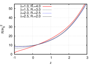
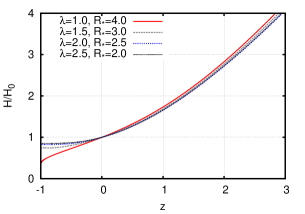
Figure 2: (color online) Ricci scalar (left panel) and the Hubble expansion (right panel) for several values of $\lambda$ and $R_{*}$ (given in units of $H_{0}^{2}$).

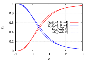
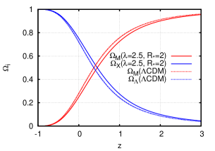
Figure 3: (color online) Evolution of $\Omega_{\rm matt}$ (red solid line) and $\Omega_{X}$ (blue solid line) for $\lambda=1$ and $R_{*}=4H_{0}^{2}$ (left panel) and $\lambda=2.5$ and $R_{*}=2H_{0}^{2}$ (right panel). For reference the corresponding quantities of the $\Lambda$CDM model are included in each panel (dashed lines).

The total EOS is defined by $\omega_{\rm tot}=(p_{\rm rad}+p_{X})/(\rho+\rho_{X})$ which using Eqs. (9) and (10) yields

$$\omega_{\rm tot}=-\frac{1}{3}\left[\frac{\frac{1}{2}\left(f_{R}R+f\right)+3f_{RR}H\dot{R}-\kappa\rho}{\frac{1}{2}\left(f_{R}R-f\right)-3f_{RR}H\dot{R}+\kappa\rho}\right]\,\,\,.$$ (11)

This EOS allows us to track the epochs where the Universe is expanding in a decelerating or accelerating fashion. If $\omega_{\rm tot}<-1/3$ then $\ddot{a}>0$, while $\ddot{a}<0$ if $\omega_{\rm tot}>-1/3$.

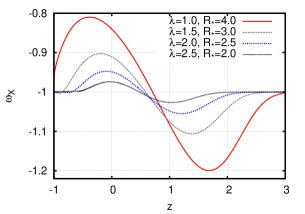
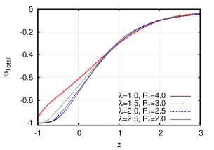
Figure 4: (color online) The EOS $\omega_{X}$ (left panel) and the total EOS $\omega_{\rm tot}$ (right panel).

4 Numerical Results and Discussion

We integrate the differential equations forward, from past to future, starting from a given $z=a_{0}/a-1$, where matter dominates, to $z\rightarrow-1$ where the GDE prevails. The initial conditions are fixed as in [11]. Figure 2 shows the Hubble expansion and the Ricci scalar for several values of $\lambda$. In all the cases where $\lambda>1$, $R$ reaches the de Sitter point at the global minimum of $V(R)$. For $\lambda=1$ because the potential is very flat around the global minimum at $R=0$, and also due to the friction term, $R$ varies very slowly as it approaches the minimum. This explains why in this case the model also mimics a cosmological constant. Figure 3 depicts the fraction of dimensionless densities $\Omega_{i}=\kappa\rho_{i}/(3H^{2})$ which satisfy the constraint $\Omega_{\rm rad}+\Omega_{\rm matt}+\Omega_{X}=1$ where $\Omega_{\rm matt}:=\Omega_{\rm bar}+\Omega_{\rm DM}$. The radiation contribution, although taken into account, is very small and cannot be appreciated from the plots. The current abundances at $z=0$ (today) match reasonably well the predicted values of the $\Lambda$CDM model and the exponential models show an adequate matter domination era. The EOS of GDE is plotted in Figure 4 (left panel), and like in other $f(R)$ models [11], it oscillates around the phantom divide value $\omega_{\Lambda}=-1$ before reaching its asymptotic value as $z\rightarrow-1$. The total EOS depicted in Figure 4 (right panel) shows that at higher $z$ the Universe is dominated by matter with $\omega_{\rm tot}\sim 0$, and then interpolates to the value $\omega_{\rm tot}=-1$ in the far future. At $z=0$, $\omega_{\rm tot}$ is similar to the value $\omega_{\rm tot}\sim 0.75$ predicted by the $\Lambda$CDM model. Figure 5 (left panel) shows the (modulus) luminous distance computed as in [11] and the deceleration parameter (right panel).

In these exponential models it is technically difficult to integrate far in the past since $f_{RR}\rightarrow 0$ exponentially. Since this quantity appears in the denominator of Eq. (6), it produces large variations that affects the precision during the numerical integration. This is something that we had encountered in other $f(R)$ models [11].

The exponential model seems to be consistent with the cosmological observations and also with the Solar System [13]. Nevertheless, like other $f(R)$ models that look viable as well, a closer examination is required in all possible scenarios before considering $f(R)$ theories as a serious threat to general relativity.

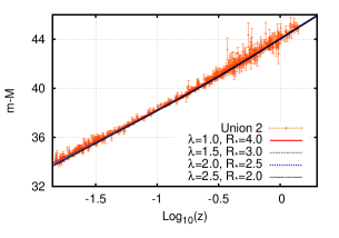
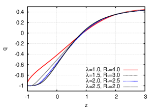
Figure 5: (color online) Luminous distance (left panel) compared with the Union 2 data [1]. Deceleration parameter (right panel).

References

References

- [1] Amanullah, R. et al., Astrophys. J., 716, 712, (2010).
- [2] Bamba, K. et al., JCAP, 08, 021, (2010).
- [3] Bianchi, E. and Rovelli, C., Nature, 466, 321, (2010). [1002.3966].
- [4] Capozziello, S. and Laurentis, M. De. [1108.6266].
- [5] Carroll, S., Living Rev. Rel., 4, 1, (2001).
- [6] Clifton, T. et al., Phys. Rep., 513, 1, (2011).
- [7] Elizalde, E. et al. [1108.6184].
- [8] Elizalde, E. et al., Phys. Rev. D, 77, 046009, (2008).
- [9] Elizalde, E. et al., Phys. Rev. D, 83, 086006, (2011).
- [10] Felice, A. De and Tsujikawa, S., Living Rev. Rel., 13, 3, (2010).
- [11] Jaime, L. G., Patino, L. and Salgado, M. [1206.1642].
- [12] Jaime, L. G., Patino, L. and Salgado, M., Phys. Rev., D83, 024039, (2011).
- [13] Linder, E. V., Phys. Rev. D, 80, 123528, (2009).
- [14] Martin, J. [1205.3365].
- [15] Miscellaneous, “Focus section on inhomogeneous cosmological models and averaging in cosmology”, Class. Quantum Grav., 28, Number 16, (2011).
- [16] Nojiri, S. and Odintsov, S. D., Phys. Rep., 505, 59, (2011).
- [17] Perlmutter, S. et al., Astrophys. J., 517, 565, (1999).
- [18] Riess, A. G. et al., Astron. J., 116, 1038, (1998).
- [19] Sahni, V. and Starobinsky, A., Int. Jour. Mod. Phys. D, 9, 373, (2000).
- [20] Sotiriou, T. P. and Faraoni, V., Rev. Mod. Phys., 82, 451, (2010).
- [21] Yang, L. et al., Phys. Rev. D, 82, 103515, (2010).
- [22] Zhang, P., Phys. Rev. D, 73, 123504, (2006).