Linear-Nonlinear-Poisson Neuron Networks Perform
Bayesian Inference On Boltzmann Machines

Abstract

One conjecture in both deep learning and classical connectionist viewpoint is that the biological brain implements certain kinds of deep networks as its back-end. However, to our knowledge, a detailed correspondence has not yet been set up, which is important if we want to bridge between neuroscience and machine learning. Recent researches emphasized the biological plausibility of Linear-Nonlinear-Poisson (LNP) neuron model. We show that with neurally plausible settings, the whole network is capable of representing any Boltzmann machine and performing a semi-stochastic Bayesian inference algorithm lying between Gibbs sampling and variational inference.

1 Introduction

Classical connectionist viewpoint has long been inspired from how the brain works, such as the invention of “perceptron” [1], and the “parallel distributed processing” approach [2]. Modern deep learning and unsupervised feature learning also assume connections between biological brain and certain kinds of deep networks, either probabilistic or not. For example, properties of visual area V2 are found to be comparable to those on the sparse autoencoder networks [3]; the sparse coding learning algorithm [4] is originated directly from neuroscience observations; also psychological phenomenon such as end-stopping is observed in sparse coding experiments [5].

In addition, there are architectural similarity between neuroscience and machine learning. For example, neuronal spike propagation may correspond to prediction or inference tasks in a learned model; synaptic plasticity may correspond to parameter estimation given the network structure; neuroplasticity may correspond to learning the network structure together with inventing new hidden units in the network; axonal path finding in the help of guidance signals may be regarded as structural priors making learning network structure easier.

For this reason, it may be helpful again to refer to how the brain works when dealing with problems that are currently puzzling machine learning researchers. For example, training deep networks was made practical mostly after the breakthrough of deep learning starting from 2006 (e.g. [6][7][8][9][10], etc.). The success may lie in a safe way of adapting the network structure, such that the parameter estimation part can be effective enough to reach non-trivial local optima. However, since the brain is not exactly layer-wise, we may wonder is there any other way of choosing the network structure along with parameter estimation? If we want to transfer neuroscience knowledge for answering questions as such and build bridge between these two areas, we want to first figure out what exactly is the deep network that the brain is representing.

A good starting point of answering this may be to look at single neuron computation. Through how they transfer information among them, we can reverse engineer both the representation and the prediction / inference algorithm, which is the main purpose of this paper.

In theoretical neuroscience, single neuron models are divided into different levels of detail, (see [11] for a five level survey). Detailed models can be quite realistic and few simplification assumptions hold. Yet effective simplification holds in different extent. For example, integrate-and-fire models capture essential properties of Hodgkin-Huxley model [12], and its variant exponential integrate-and-fire neuron models [13] are found to be capable of reproducing spike timing of several types of cortical neurons. The community has also been investigating on the Linear-Nonlinear-Poisson (LNP) models for long [14][15][16]. A recent study in [17] analyzed how LNP models effectively reproduce firing rates in more realistic neurons. Based on these results, we start from formally presenting the LNP model and then turn to presenting a semi-stochastic inference algorithm on Boltzmann machines, which is derived from combining Gibbs sampling and variational inference. We then make a detailed matching between LNP model and the inference algorithm. Since the semi-stochastic inference algorithm has not been explored in the learning community, we also show some experiments illustrating its computational property, including its stochastic convergence and its similarity to variational inference.

2 Brief Review on Neural Plausibility of LNP Model

In this section, we briefly review the Linear-Nonlinear-Poisson neuron model and its neural plausibility, focusing on what modeling options we have to fit it with useful inference algorithms.

The LNP neuron model [14][15][16] formalizes the spike train generated by each neuron as a non-homogeneous Poisson point process, whose rate function over time depends on the input spike trains from its presynaptic neurons, with certain form of short-term memory in the dependence.

$$\begin{gathered}{\text{Synaptic Transmission: }\text{ }\text{ }\text{ }}{I_{ij}}\left(\tau\right)={W_{ij}}\cdot\left({{X_{j}}*\alpha}\right)\left(\tau\right)\text{ }\text{ }\text{ }\text{ }\text{ }\text{ }\text{ }\text{ }\text{ }\text{ }\text{ }\text{ }\text{ }\text{ }\text{ }\text{ }\text{ }\text{ }\text{ }\text{ }\text{ }\text{ }\text{ }\text{ }\text{ }\text{ }\text{ }\text{(a)}\hfill\\ {\text{Dendritic Integration: }\text{ }\text{ }\text{ }\text{ }\text{ }}{I_{i}}\left(\tau\right)={\text{Multi - Linear}}\left({{{\left\{{{I_{ij}}\left(\tau\right)}\right\}}_{j\in M\left(i\right)}}}\right)\text{ }\text{ }\text{ }\text{ }\text{ }\text{ }\text{(b)}\hfill\\ {\text{Spike Generation: }\text{ }\text{ }\text{ }\text{ }\text{ }\text{ }\text{ }\text{ }\text{ }\text{ }}\left\{\begin{gathered}{\lambda_{i}}\left(\tau\right)=\sigma\left({\left({{I_{i}}*D}\right)\left(\tau\right)}\right)\hfill\text{ }\text{ }\text{ }\text{ }\text{ }\text{ }\text{(c)}\\ {X_{i}}\left(\tau\right)\sim{\text{PoissonPointProcess}}\left({{\lambda_{i}}\left(\tau\right)}\right)\hfill\text{ }\text{ }\text{ }\text{ }\text{ }\text{ }\text{ }\text{ }\text{(d)}\\ \end{gathered}\right.\hfill\\ \end{gathered}$$ (1)

In all these equations, $\tau$ is the continuous time index, whose unit is millisecond. Subscript $i$ is the index of the neuron in question, $M\left(i\right)$ is the index set of presynaptic neurons of neuron $i$. In Eq. (1)(d), ${X_{i}}\left(\tau\right)=\sum\nolimits_{f}{\delta({\tau-\tau_{i}^{\left(f\right)}})}$ represents the spike train, with spikes as Dirac functions located at time steps $\tau_{i}^{\left(f\right)}$. $\lambda_{i}\left(\tau\right)$ is the rate function of the Poisson point process. Eq. (1)(a) represents the postsynaptic current at a particular synapse with efficacy $W_{ij}$. $\alpha$ is a certain non-negative function with certain time course. Evidence for “Poisson-like” statistics in cortical neurons can be found in [18][19], which implies that spike counts over a certain interval may be Poisson distributed.

Eq. (1)(b) is the dendritic summation. There are different viewpoints on whether linearity holds true. Due to phenomenon like mutual inhibition on different dendritic shafts, it is commonly known that nonlinear summation could happen (see [20][21] for example), yet studies from [22] show that when dendritic spines are presented, linear summation is true, and this happens frequently in excitatory mammalian cortex. In addition, a survey on neuron models in [11] summarized different computations that can be performed in dendritic processing, two notable examples are multiplication and summation. We include these two and generalizes them into the “Multi-Linear” function in Eq. (1)(b), i.e., it is linear with respect to each of its arguments individually. Here we use the set notation $\left\{\cdot\right\}_{j\in M\left(i\right)}$ to denote the set of arguments. What is special in a “Multi-Linear” function is that, when taking its expectation with respect to a certain argument, the expectation goes in and the resulted formula simply replaces the argument by its mean. This is useful for mean-field algorithms.

After dendritic summation, relationship between the summed current and the firing rate can be well researched by in-vitro neuroscience experiments where input current can be externally controlled. Various frequency-current function can also be derived from popular spike generation models, such as Leaky Integrate-and-Fire model (see [12] for an overview), Exponential Integrate-And-Fire Model [13], Spike Response Model [23], or more realistic models such as Hodgkin-Huxley Model [24]. In particular, [14][15][16] formulated the LNP simplification through a nonlinear mapping followed by a Poisson point process random sampling. The analytical study with simulation in [17] show that the simplification is effective. We put this in Eq. (1)(c).

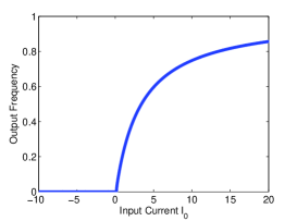
Figure 1: Frequency-current curve of leaky integrate-and-fire neurons for a particular set of parameters. More from different neuron models can be found in [12].

Since neural spikes has refractory period with at least 1ms, firing rate will not exceed 1000Hz and there won’t be more than one spike happening in 1ms, so $\lambda_{i}\left(\tau\right)\in\left[0,1\right]$. In practice, firing rate is often even lower. In addition, discrete time steps in the resolution of 1ms per each step seems quite fine-grained for most perceptual tasks (e.g., visual recognition emerges in 75-80ms [25]). For these reasons, discretizing time into 1ms per each step may be reasonable. By LeCam’s theorem [26], the discrete counterpart of nonhomogeneous Poisson point process is the nonhomogeneous Bernoulli process, and the Bernoulli probability at each discrete time step is approximated by the integration of rate function at that time period. We use $t\in\mathbb{Z}$ to denote the discrete time steps, whose unit is millisecond. We use $\phi_{i}^{\left(t\right)}\in\left[0,1\right]$ to denote the Bernoulli probability and $x_{i}^{\left(t\right)}\in\left\{0,1\right\}$ to denote the spike indicator at time $t$,

$$x_{i}^{\left(t\right)}\sim{\text{Bernoulli}}\left({\phi_{i}^{\left(t\right)}}\right),{\text{ }\text{ }\text{ }}\phi_{i}^{\left(t\right)}\triangleq\int_{t}^{t+1}{{\lambda_{i}}\left(\tau\right)d\tau}$$ (2)

The corresponding discrete form of Eq. (1)(a,b,c) is by substituting $X_{i}\left(\tau\right)$ with $x_{i}^{\left(t\right)}$ and substituting $\alpha$, $D$ functions with their discrete form similar to the definition of $\phi_{i}^{\left(t\right)}$ in Eq. (2). There are two ways to proceed with the formulation. In case $D$ function is the Dirac function located at 0, or is close to that, the convolution with $D$ can be ignored, the discrete counterpart of Eq. (1)(a,b,c) are

$$\begin{gathered}I_{ij}^{\left(t\right)}={W_{ij}}\cdot\sum\nolimits_{k=1}^{K_{\alpha}}{\alpha\left(k\right)\cdot x_{i}^{\left({t-k}\right)}}\hfill\\ \phi_{i}^{\left(t\right)}=\sigma\left({{\text{Multi-Linear}}\left({{{\left\{{I_{ij}^{\left(t\right)}}\right\}}_{j\in M\left(i\right)}}}\right)}\right)\hfill\\ \end{gathered}$$ (3)

Or if $D$ is non-trivial, but the Multi-Linear function in Eq. (1)(b) reduces to a linear summation, by the associativity of convolution, we can let $\epsilon=\alpha*D$, and the discrete counterpart of Eq. (1)(a,b,c) reduces to the following, assuming finite time course of the function $\epsilon$.

$$\phi_{i}^{\left(t\right)}=\sigma\left({\sum\nolimits_{j\in M\left(i\right)}{{W_{ij}}\cdot\sum\nolimits_{k=1}^{K}{\epsilon\left(k\right)\cdot x_{i}^{\left({t-k}\right)}}}}\right)$$ (4)

In [17], $D$ functions resulted from spiking neuron models are not Dirac functions, but are very close. In the latter part of this paper, we will focus on the case when linear summation is true (hence Eq. (4) holds) although multi-linearity in Eq. (3) may generalize our formulation to high-order Boltzmann machines. Another observation is that in Eq. (4), if $D$ is exponential function (true in [17]) and $\alpha$ is exponential function too (true in [12]), and assuming both functions have the same scale parameter, $\epsilon$ becomes the classic $\alpha$-function [27] used in postsynaptic modeling.

Another issue is whether linear summation in Eq. (4) or multi-linear integration in Eq. (3) contains a constant bias term $b_{i}$. In [28], there is such a bias term in the spiking response model. This will make our latter part easier, but in our derivation later, we focus on the case when there is no such bias. It will be trivial then to turn to the case where bias exists.

To sum up, the LNP neuron model we are going to deal with in the latter part is as the following, assuming $\mathcal{H}$ is the index set of neurons whose activity is not bound to observations (external stimuli).

$${\text{For all }}i\in\mathcal{H},t\in{\mathbb{Z}^{+}},{\rm{}}\left\{\begin{array}[]{l}x_{i}^{\left(t\right)}\sim{\rm{Bernoulli}}\left({\phi_{i}^{\left(t\right)}}\right)\\ \phi_{i}^{\left(t\right)}=\sigma\left({\sum\nolimits_{j\in M\left(i\right)}{{W_{ij}}\cdot\sum\nolimits_{k=1}^{K}{\epsilon\left(k\right)\cdot x_{i}^{\left({t-k}\right)}}}}\right)\end{array}\right.$$ (5)

$\sigma$ function can be fit from data or from realistic neuron models, and has some relationship with the frequency-current curve. According to [12][17], such nonlinearity in different spiking neuron models may be non-decreasing, close to zero towards the left, increase almost linearly in a certain interval. Also, since firing rate has upper bounds, $\sigma$ won’t increase unboundedly. For this reason, $\sigma$ may be considered as a modification of sigmoid function to meet certain demands of inference. An example of frequency-current curve is shown in Fig. 1. See also [17] for another type of nonlinearity. In Fig. 1, parameters of the leaky integrate-and-fire model are set as ${\tau_{m}}=20{\text{ ms, }}{\Delta^{{\text{abs}}}}=1{\text{ ms, }}R=1{\text{ m}}\Omega{\text{, }}\upsilon=1{\text{ mV}}$ (with notations following [12]).

In the biological brain, all neurons are computing in parallel. Thus we want to investigate on the case when Eq. (5) is executed in parallel, vectors ${{\mathbf{x}}^{\left(t\right)}}=({x_{i}^{\left(t\right)}})_{i=1}^{n}$ and ${{\mathbf{\phi}}^{\left(t\right)}}=({\phi_{i}^{\left(t\right)}})_{i=1}^{n}$ over time forms a Markov chain of order $K$. The latter part focuses on showing its stochastic inference nature.

3 Semi-Stochastic Inference on Boltzmann Machines

In this section, first we compare Gibbs sampling and variational inference on Boltzmann machines, emphasizing their architectural similarity, then we present the semi-stochastic inference algorithm by combining them. Some notations we use in this section will overlap with the last section. This is intended since we want to link the quantities in both sections.

Let ${\rm{\bf Y}}\in\left\{{A,B}\right\}^{n}$ be a collection of random variables. Each of them has two possible values $A$ and $B$ (e.g., $A=0$ and $B=1$ in the binary case). Let $\mathcal{V},\mathcal{H}$ be a partition of the index set $\mathcal{I}=\left\{{1,...,n}\right\}$. We denote $Y_{\mathcal{V}}$ as the visible variables, $Y_{\mathcal{H}}$ as the hidden variables. We use lower case of $Y$ to denote its values, e.g., $y_{i}$, $y_{\mathcal{H}}$ or $\mathbf{y}$. In this paper we use the Boltzmann machines with softmax units [29],

$$p\left({\bf{y}}\right)=\frac{1}{Z}\exp\left({\frac{1}{2}\cdot\sum\limits_{i,j:i\neq j;u,v\in\left\{{A,B}\right\}}{\left[\kern-1.49994pt\left[{{y_{i}}=u}\right]\kern-1.49994pt\right]\cdot\left[\kern-1.49994pt\left[{{y_{i}}=v}\right]\kern-1.49994pt\right]\cdot{V_{iu,jv}}}-\sum\limits_{i\in{\cal I},u\in\left\{{A,B}\right\}}{\left[\kern-1.49994pt\left[{{y_{i}}=u}\right]\kern-1.49994pt\right]\cdot{c_{iu}}}}\right)$$ (6)

Here we denote $\left[\kern-1.49994pt\left[\cdot\right]\kern-1.49994pt\right]$ as the binary indicator. $\left[\kern-1.49994pt\left[\cdot\right]\kern-1.49994pt\right]=1$ if the statement is true and $\left[\kern-1.49994pt\left[\cdot\right]\kern-1.49994pt\right]=0$ otherwise. ${\rm{\bf V}}=\left({V_{iu,jv}}\right)_{i,u,j,v}$ is a four-dimensional tensor of size $4n^{2}$, ${\rm{\bf c}}=\left({c_{iu}}\right)_{i,u}$ is a matrix of size $2n$. $Z$ is the normalization constant (partition function), which depends on ${\rm{\bf V}}$ and ${\rm{\bf c}}$. Note that this family has no more capacity than the original Boltzmann machine [30] and the Ising model [31].

In Gibbs sampling without parallelism [32][33], we are given an observed value $y_{\mathcal{V}}$, and we want to find a sequence $\left\{y_{\mathcal{H}}^{\left(t\right)}\right\}_{t=0}^{\infty}$ which converges in distribution to the true posterior $p\left(Y_{\mathcal{H}}|Y_{\mathcal{V}}=y_{\mathcal{V}}\right)$. The algorithm proceeds as follows. First we initialize $y_{\mathcal{H}}^{\left(0\right)}$, and let $y_{\mathcal{V}}^{\left(0\right)}$ take on the observed values. Then at each iteration $t\in\mathbb{Z}^{+}$ we pick an index $i\in\mathcal{H}$ and do the following,

(a) $$\text{Calculate proposal }{\phi_{iu}^{\left(t\right)}=\sigma\left({\sum\nolimits_{j\in M\left(i\right),v\in\left\{A,B\right\}}{W_{iu,jv}\cdot\left[\kern-3.00003pt\left[y_{j}^{\left({t-1}\right)}=v\right]\kern-3.00003pt\right]}-b_{iu}}\right),\forall u\in\left\{A,B\right\}}$$ (7)

(b) $$\text{Sample }y_{i}^{\left(t\right)}\sim\mbox{Bernoulli}\left({\phi_{iA}^{\left(t\right)},\phi_{iB}^{\left(t\right)}}\right)\text{, pass down samples by }y_{\sim i}^{\left(t\right)}=y_{\sim i}^{\left({t-1}\right)}$$

Here we denote $W_{iu,jv}=V_{iu,jv}-V_{i\bar{u},jv}$ and $b_{iu}=c_{iu}-c_{i\bar{u}}$ with $\bar{u}$ defined as $\left\{{\bar{u}}\right\}=\left\{{A,B}\right\}\backslash\left\{u\right\}$. $\sigma\left(x\right)=1/\left({1+\exp\left({-x}\right)}\right)$ is the sigmoid function. $M\left(i\right)$ is the index set of Markov blanket of $Y_{i}$, $i.e.$, $M\left(i\right)=\left\{{j\in\mathcal{I}|j\neq i,\exists u,v\in\{A,B\},\text{s.t. }V_{iu,jv}\neq 0}\right\}$.

Variational inference with factorized approximation family often takes the form of a mean-field version of Gibbs sampling (e.g.,  [34]). We adopt the same family of variational distributions as in [35], such that $q\left({{Y_{\mathcal{H}}}|{\Theta_{\mathcal{H}}}}\right)=\prod\nolimits_{i\in{\mathcal{H}}}{q\left({{Y_{i}}|{\theta_{iA},\theta_{iB}}}\right)}$, where each $q\left({Y_{i}|\theta_{iA},\theta_{iB}}\right)$ is a Bernoulli distribution such that $\theta_{iu}=q\left({Y_{i}=u|\theta_{iA},\theta_{iB}}\right)$ for $u\in\left\{A,B\right\}$. The objective of variational inference is to find $\Theta_{\mathcal{H}}$ by minimizing the loss function $L\left({\Theta_{\mathcal{H}}}\right)=KL\left({q\left({{\rm{\bf Y}}|{\rm{\bf\Theta}}}\right)||p\left({{\rm{\bf Y}}}\right)}\right)$, here $KL\left({q||p}\right)=E_{q}\log\left({q/p}\right)$ is the KL-divergence.

The algorithm proceeds as: first we randomly initialize $\Theta_{\mathcal{H}}^{\left(0\right)}$, then at each iteration $t\in\mathbb{Z}^{+}$ we pick an index $i\in\mathcal{H}$ and do the following,

(a) $$\text{Calculate update }\phi_{iu}^{\left(t\right)}=\sigma\left({\sum\nolimits_{j\in M\left(i\right),v\in\left\{A,B\right\}}{W_{iu,jv}\cdot\theta_{jv}^{\left({t-1}\right)}}-b_{iu}}\right),\forall u\in\left\{A,B\right\}$$ (8)

(b) $$\text{Assign }\theta_{iu}^{\left(t\right)}=\phi_{iu}^{\left(t\right)}\text{, pass down }\theta_{\sim iu}^{\left(t\right)}=\theta_{\sim iu}^{\left({t-1}\right)},\forall u\in\left\{A,B\right\}.$$

Our motivation for combining them is as follows. First, exponential family distributions have sufficient statistics [36]. By accumulating the empirical expectation of sufficient statistics, we can online estimate the parameter if data instances are completely observed, e.g., to online estimate a Gaussian distribution $\mathcal{N}\left(X|\mu,\sigma\right)$, we can incrementally calculate $\sum\nolimits_{i=1}^{t}{{x_{i}}}$ and $\sum\nolimits_{i=1}^{t}{x_{i}^{2}}$, and estimate $\hat{\mu}$ and $\hat{\sigma}$ at each time $t$ by only using these two statistics.

Now if we take the examples in Gibbs sampling as the online data instances and estimate a distribution from within the variational approximation family, we will end up getting a marginal probability distribution for each random variable (when mixing is good). However, we can also change the way how the sequence is generated, such that the online estimated variational distribution biases towards whatever we want. In particular, we can take the calculated distribution in Eq. (8)(a) as the proposal distribution, used to sample a new data example, and incrementally update the variational distribution by using that. The updated variational distribution serve as the next input to Eq. (8). If decaying as in [37] is used when accumulating sufficient statistics, the variational distribution estimated in our Bernoulli case, is simply a weighted sum of the most recent examples:

$$\theta_{iu}^{\left(t\right)}=\sum\nolimits_{k=0}^{-\infty}{\epsilon\left(k\right)\cdot\left[\kern-3.00003pt\left[{y_{i}^{\left({t-k}\right)}=u}\right]\kern-3.00003pt\right]},{\text{ for }}u\in\left\{{A,B}\right\}$$ (9)

The $-\infty$ in Eq. (9) simply means the starting time of accumulation. $\epsilon$ function is non-negative and should sum up to one for all $k$ in the effective time span. In case constant decaying ratio is used on the last accumulated sufficient statistics as in [37], the $\epsilon$ function above decays exponentially. Some choices of $\epsilon$ function may not have any online updating scheme that produces it. In practice, we can either do online updating or let $\epsilon$ have a finite time course, up to some $K\in\mathbb{Z}^{+}$.

In semi-stochastic inference, we choose a non-negative weight function ${\rm{\epsilon}}\left(k\right)$ which sum up to 1 for $k\in\left\{1,2,...,K\right\}$. We initialize both ${\rm{\bf y}}^{\left(0\right)}$ and ${\rm{\bf\Theta}}^{\left(0\right)}$. In each iteration $t\in\mathbb{Z}^{+}$ we pick an index $i\in\mathcal{H}$ and do the following,

(a) $$\phi_{iu}^{\left(t\right)}=\sigma\left({\sum\nolimits_{j\in M\left(i\right),v\in\left\{{A,B}\right\}}{{W_{iu,jv}}\cdot\theta_{jv}^{\left(t-1\right)}}-{b_{iu}}}\right),\text{ for }u\in\left\{{A,B}\right\}$$

(b) $$y_{i}^{\left(t\right)}\sim\mbox{Bernoulli}\left({\phi_{iA}^{\left(t\right)},\phi_{iB}^{\left(t\right)}}\right)$$

(c) $$\theta_{iu}^{\left(t\right)}=\sum\nolimits_{k=1}^{K}{\epsilon\left(k\right)\cdot\left[\kern-3.00003pt\left[{y_{i}^{\left({t-k+1}\right)}=u}\right]\kern-3.00003pt\right]},\text{ for }u\in\left\{{A,B}\right\}$$

In sequential inference, for every other random variable which does not carry out these updating steps, we will pass down $\theta$ and most recent $K$ copies of $y$’s to the next time step. In step (c), additional normalization is needed when $t<K$. Details are ignored for clarity of presentation.

In another way, we can also look at algorithm in Eq. (3) as a “random slowing-down” / stochastic approximation / momentum version of variational inference. When an updated variational distribution is computed, we don’t immediately turn to the updated distribution. Instead, we use it to sample a new example, and use it to incrementally update the original variational distribution. The expectation of the new example will be the same as the updated variational distribution.

4 Making Detailed Correspondence

To connect LNP neuron model in Eq. (5) with semi-stochastic inference algorithm in Eq. (3), several issues needs to be resolved:

1. LNP neurons don’t have the bias terms (such as $b_{iu}$), although their nonlinear transform function may have constant shift identical to all neurons.

2. In Eq. (3), two Linear-Nonlinear procedures in (a)(c) corresponds to only one sampling step in (b). This is an architectural difference.

3. Biological neurons can only be excitatory or inhibitory.

4. Biological neurons carry out the updates all in parallel.

To resolve issue 1, we notice that when the weights $\mathbf{V}$ and biases $\mathbf{c}$ in Eq. (6) are turned into $\mathbf{W}$ and $\mathbf{b}$ in Eq. (3), for fixed $i,j\in\mathcal{I}$, fixed $u,v\in\left\{A,B\right\}$, and any constant $C\in\mathbb{R}$ the following operation is invariant to the inference algorithm in Eq. (3) since $\theta_{iA}^{\left(t\right)}$ and $\theta_{iB}^{\left(t\right)}$ sum up to one.

$$\left\{\begin{gathered}b_{iu}^{\text{new}}\leftarrow b_{iu}^{\text{old}}+C\hfill\\ W_{iu,jv}^{\text{new}}\leftarrow W_{iu,jv}^{\text{old}}+C\hfill\\ W_{iu,j\bar{v}}^{\text{new}}\leftarrow W_{iu,j\bar{v}}^{\text{old}}+C\hfill\\ \end{gathered}\right.$$ (11)

For this reason, we can always modify the algorithm in Eq. (3) to make any bias we want. In our experiments, when we want to remove a bias $b_{iu}$, we subtract $b_{iu}/{|M\left(i\right)|}$ from both $W_{iu,jv}$ and $W_{iu,j\bar{v}}$ for each $j\in M\left(i\right)$.

To resolve issue 2, we propose the “Event-Network”. We first split every sampling step (b) in Eq. (3) into two, namely $[\kern-1.49994pt[{y_{i}^{\left(t\right)}=A}]\kern-1.49994pt]\sim\mbox{Bernoulli}({\phi_{iA}^{\left(t\right)}})$ and $[\kern-1.49994pt[{y_{i}^{\left(t\right)}=B}]\kern-1.49994pt]\sim\mbox{Bernoulli}({\phi_{iB}^{\left(t\right)}})$. Now we can allocate two neurons to take care of the two parts in all three steps (a)(b)(c). Units of the resulted network no longer corresponds to random variables, they are now probabilistic events. When we do this, there is no guarantee that $\theta_{iA}^{\left(t\right)}$ and $\theta_{iB}^{\left(t\right)}$ will sum up to 1, but this will be approximately true since the weights $W_{iu,jv}$’s are compatible with each other. Whether this results in meaningful inference algorithms needs further investigation. We show verification in our experiment part.

To resolve issue 3, once we have a network containing neurons with both excitatory and inhibitory outgoing synapses, we can duplicate each neuron into two, both have the same incoming synapses with the original neural efficacy. Then one of them take all positive outgoing synapses before splitting, and the other take all negative ones. Both of this and the last modification of the network are exactly invariant for variational inference but may only be approximately true for semi-stochastic inference. We show experimental verification for this modification as well.

If after resolving all these issues we denote $x_{iu}^{\left(t\right)}=[\kern-1.49994pt[{y_{i}^{\left(t\right)}=u}]\kern-1.49994pt]$ for $u\in\left\{A,B\right\}$, and re-index everything, the resulted algorithm will be exactly the same as Eq. (5) if executed in parallel. Parallelism is not only an issue in semi-stochastic inference. It is noticed in [33] that when adjacent random variables of a Boltzmann machine are updated in parallel in Gibbs sampling, the sample sequence does not converge to the right distribution. This issue is also raised very often recently (e.g. [38]). Variational inference is a fixed point iteration. So it may converge to the same answer when updated all in parallel, but we do observed experimentally that the variational parameters converges to the fixed point after severe oscillation. Whether the slowing down version alleviates this problem requires further investigation.

5 Experimental Verification

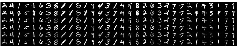
Figure 2: Samples of reconstruction results (selected randomly). Rows from top to bottom: original images; VarO; SemiO; SemiEN; SemiB; SemiU.

In this section, we focus on illustrating that the semi-stochastic inference, as well as all the modifications in section 4, are valid Bayesian inference algorithms, which behave similar to variational inference. In all experiments, we set $\epsilon(k)$ as $\exp(-k/2)$ normalized to have summation 1 over its domain $k\in\left\{1,...,30\right\}$. All inferences are carried out in synchronized full parallelism.

To avoid the complication of learning deep Boltzmann machines, we take the learned Boltzmann machine from code in [35]. Since we focus on inference on Boltzmann machine, we take the learned model before back-propagation. The Boltzmann machine we use consists of three layers, the first layer for input image consists of 784 units, the second consists of 500 units and the third consists of 1000 units. In the following, we refer to $\theta_{i}^{(t)}$ in both algorithms as the activation of neuron $i$.

To see the effect of modifications in section 4, we show results of semi-stochastic inference after each of them. Note that variational inference is exactly invariant on all these modifications, hence there no need to verify them. We use the following abbreviations in this part:

• VarO: variational inference applied on the original deep Boltzmann machine.

• SemiO: semi-stochastic inference applied on the original deep Boltzmann machine.

• SemiEN: Same as SemiO except each sampling is duplicated and put on two neurons.

• SemiB: Same as SemiEN except biases are removed by transforming the network.

• SemiU: Same as SemiB except each neuron is duplicated into two, such that no neuron contains out-going synapses with different signs.

The experiment we did is similar to the reconstruction experiment in [7]. We do the following: (i) plug in an image on the input layer, (ii) apply the inference algorithm, (iii) frozen the activations on the topmost layer and round up to 0 or 1, (iv) set the topmost layer as observed and other layers as hidden, (v) infer back, (vi) read off the image as activations on the input layer. Both (ii) and (v) are randomly initialized and have 100 iterations. For semi-stochastic inference, in steps (iii) and (vi) the activations are taken as averages over the last 50 iterations, while for variational inference we simply use the last activation of each neuron. This is because semi-stochastic inference has random convergence, activations approach some fixed point with random perturbation (see justification later). Some reconstruction examples are shown in Fig. 2. Each algorithm has good and bad cases, also note that because of the randomness, even for identical input image and identical initialization, semi-stochastic inference may get different results in different trials.

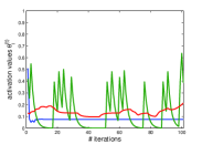
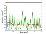
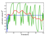
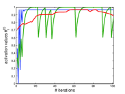
Figure 3: Sample trajectory of $\theta_{i}^{(t)}$ in VarO and SemiO. In all above, Blue line is for VarO, Green line is for SemiO, and Red line is the moving average of Green line over window size 30.

In figure 3, we showed sample trajectory of activations in step (ii) of VarO and SemiO for the same variables. Each trajectory are those $\theta_{i}^{(t)}$’s of one neuron over all iterations. We see that activations in variational inference converge to a stable solution with oscillation before convergence, while semi-stochastic inference has their moving average converges to some similar values with random perturbation. Figure 5(a) is a scatter plot of mean of trajectories vs. the corresponding converged activation in variational inference, extracted from 2000 trajectories randomly chosen from 50 trials. We also observed that when the mean is close to extreme values (such as 0 and 1), the standard variance will be smaller, as can be found in figure 3 and more clearly in figure 5(b). This means that semi-stochastic inference converges randomly to the variational inference solution, with more confident variables having less random perturbation.

Finally, we investigated on how well the splitting in section 4 preserves identity relationships that are expected on SemiU. In particular, if two neurons are resulted from splitting one sampling into two in resolving issue 2, their summed activation should be close to 1. If two neurons are resulted from splitting one neuron into two in resolving issue 3, their activation should be equal. Figure 4 illustrated three samples and histogram on 2000 random trajectories are given in figure 5(c)(d).

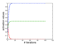
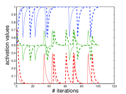
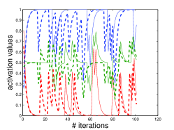
(a)	(b)	(c)

Figure 4: Sample trajectory from SemiU. Each plot shows four neurons resulted from two splits on a single neuron. Thick dash lines: neurons with positive outgoing weights. Thin solid lines: corresponding neurons with negative outgoing weights. Blue and Red lines are for the two neurons from splitting one sampling into two. Green line is the average of Blue and Red. Ideally, lines with same color should be equal, and green lines should be at 0.5.

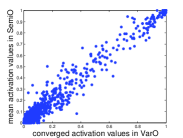
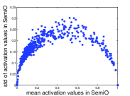
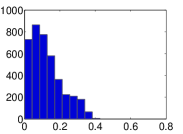
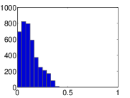
(a)	(b)	(c)	(d)

Figure 5: Some statistics of the algorithms. (a) means of trajectories in SemiO vs. converged activation values in VarO for the same hidden variables. (b) standard deviation vs. mean, from the trajectories in SemiO. (c) histogram of standard_deviation(red line + blue line - 1.0). (d) histogram of standard_deviation(dash line - solid line). (Here red, blue, dash, solid lines refer to figure 4.)

6 Conclusions and Discussions

We pointed out the stochastic inference nature of the LNP neuron models, which may serve as an interpretation of neural coding. The stochastic convergence seems reasonable, e.g., when we see ambiguous images, our perception will switch back and forth between plausible explanations.

There are many behavioral experiments showing statistical optimality of perception and learning (e.g. [39]) and many calls for neuronal modeling that achieves this optimality (e.g. [40]). Arguably, the mode-seeking nature of variational inference [41] make it natural for interpreting perception. Since Boltzmann machines with hidden variables are universal approximators (e.g. [42]), modeling knowledge representation by that is safe if the world can be approximately binarized. Yet we only show that with particular choices of weights, neurons are capable of representing a Boltzmann machine and carry out inference. Then the question is what does this do if the network is a recurrent neural network in general. Real biological neural networks may be learned by taking the Boltzmann machine representation and undergoing discriminative training or reinforcement learning to optimize performance of inference directly (especially plausible when time dimension is involved), which yields a model not necessarily convey consistent probabilistic semantics but may do so in the limit. The particular form of nonlinearity in biological neurons may also result from such optimization. Another issue is the low average activity in biological neurons. It may be a certain form of sparse coding [4] on top of inference so that optimizing such inference procedure will not yield degenerate solution. In this case, likelihood-based learning such as contrastive divergence may still be applicable as a further refinement.

References

- [1] Frank Rosenblatt. The perceptron: a probabilistic model for information storage and organization in the brain. pages 89–114, 1988.
- [2] David E Rumelhart, James L Mcclelland, and Geoffrey E Hinton. Parallel Distributed Processing: Explorations in the Microstructure of Cognition. MIT Press, August 1986.
- [3] Honglak Lee, Chaitanya Ekanadham, and Andrew Y. Ng. Sparse deep belief net model for visual area V2. In Advances in Neural Information Processing Systems 20, pages 873–880. 2008.
- [4] Bruno. A. Olshausen and David J. Field. Emergence of simple-cell receptive field properties by learning a sparse code for natural images. Nature, 381:607–609, 1996.
- [5] Honglak Lee, Alexis Battle, Rajat Raina, and Andrew Y. Ng. Efficient sparse coding algorithms. In Advances in Neural Information Processing Systems 19, pages 801–808. 2007.
- [6] Geoffrey E. Hinton, Simon Osindero, and Yee-Whye Teh. A fast learning algorithm for deep belief nets. Neural Comput., 18(7):1527–1554, July 2006.
- [7] Geoffrey E. Hinton and Ruslan R. Salakhutdinov. Reducing the dimensionality of data with neural networks. Science, 313(5786):504–507, 2006.
- [8] Yoshua Bengio, Pascal Lamblin, Dan Popovici, and Hugo Larochelle. Greedy layer-wise training of deep networks. In B. Schölkopf, J. Platt, and T. Hoffman, editors, Advances in Neural Information Processing Systems 19, pages 153–160. MIT Press, Cambridge, MA, 2007.
- [9] Quoc Le, Marc’Aurelio Ranzato, Rajat Monga, Matthieu Devin, Kai Chen, Greg Corrado, Jeff Dean, and Andrew Ng. Building high-level features using large scale unsupervised learning. In Proceedings of the Twenty-Ninth International Conference on Machine Learning, 2012.
- [10] Honglak Lee, Roger Grosse, Rajesh Ranganath, and Andrew Y. Ng. Convolutional deep belief networks for scalable unsupervised learning of hierarchical representations. In Proceedings of the 26th Annual International Conference on Machine Learning, ICML ’09, pages 609–616, New York, NY, USA, 2009. ACM.
- [11] Andreas V. M. Herz, Tim Gollisch, Christian K. Machens, and Dieter Jaeger. Modelling single-neuron dynamics and computations: A balance of detail and abstraction. Science, 314:80–84, October 2006.
- [12] Wulfram Gerstner and Werner M. Kistler. Spiking Neuron Models: Single Neurons, Populations, Plasticity. Cambridge University Press, 1 edition, 2002.
- [13] Nicolas Fourcaud-Trocm , David Hansel, Carl van Vreeswijk, and Nicolas Brunel. How spike generation mechanisms determine the neuronal response to fluctuating inputs. The Journal of Neuroscience, 23(37):11628–11640, 2003.
- [14] E. J. Chichilnisky. A simple white noise analysis of neuronal light responses. Network (Bristol, England), 12(2):199–213, May 2001.
- [15] Eero P. Simoncelli, Liam Paninski, Jonathan Pillow, and Odelia Schwartz. Characterization of neural responses with stochastic stimuli. The cognitive neurosciences, 2004.
- [16] Liam Paninski. Maximum likelihood estimation of cascade point-process neural encoding models. Network: Comput. Neural Syst., 15(04):243–262, November 2004.
- [17] Srdjan Ostojic and Nicolas Brunel. From spiking neuron models to Linear-Nonlinear models. PLoS Comput Biol, 7(1):e1001056+, January 2011.
- [18] David J. Tolhurst, J. A. Movshon, and A. F. Dean. The statistical reliability of signals in single neurons in cat and monkey visual cortex. Vision Research, 23(8):775–785, 1983.
- [19] Wei J. Ma, Jeffrey M. Beck, Peter E. Latham, and Alexandre Pouget. Bayesian inference with probabilistic population codes. Nature Neuroscience, 9(11):1432–1438, October 2006.
- [20] Idan Segev. What do dendrites and their synapses tell the neuron? Journal of Neurophysiology, 95(3):1295–1297, March 2006.
- [21] Idan Segev and Michael London. Dendritic processing. In Michael A. Arbib, editor, The handbook of brain theory and neural networks, pages 324–332. MIT Press, Cambridge, MA, USA, 2003.
- [22] Roberto Araya, Kenneth B. Eisenthal, and Rafael Yuste. Dendritic spines linearize the summation of excitatory potentials. Proceedings of the National Academy of Sciences of the United States of America, 103(49):pp. 18799–18804, 2006.
- [23] W. Gerstner. Spike-response model. Scholarpedia, 3(12):1343, 2008.
- [24] Alan L. Hodgkin and Andrew F. Huxley. A quantitative description of membrane current and its application to conduction and excitation in nerve. The Journal of Physiology, 117(4):500–544, 1952.
- [25] Rufin Vanrullen and Simon J. Thorpe. The time course of visual processing: From early perception to decision-making. J. Cognitive Neuroscience, 13(4):454–461, May 2001.
- [26] Lucien le Cam. An approximation theorem for the poisson binomial distribution. Pacific Journal of Mathematics, 10:1181–1197, 1960.
- [27] Wilfrid Rall. Distinguishing theoretical synaptic potentials computed for different soma-dendritic distributions of synaptic input. Journal of neurophysiology, 30(5):1138–1168, September 1967.
- [28] Danilo J. Rezende, Daan Wierstra, and Wulfram Gerstner. Variational learning for recurrent spiking networks. In J. Shawe-Taylor, R.S. Zemel, P. Bartlett, F.C.N. Pereira, and K.Q. Weinberger, editors, Advances in Neural Information Processing Systems 24, pages 136–144. 2011.
- [29] Ruslan Salakhutdinov and Geoffrey Hinton. Replicated softmax: an undirected topic model. In Y. Bengio, D. Schuurmans, J. Lafferty, C. K. I. Williams, and A. Culotta, editors, Advances in Neural Information Processing Systems 22, pages 1607–1614. 2009.
- [30] David H. Ackley, Geoffrey E. Hinton, and Terrence J. Sejnowski. A Learning Algorithm for Boltzmann Machines. Cognitive Science 9, pages 147–169, 1985.
- [31] Ernst Ising. Beitrag zur theorie des ferromagnetismus. Zeitschrift f r Physik A Hadrons and Nuclei, 31:253–258, 1925. 10.1007/BF02980577.
- [32] Stuart Geman and Donald Geman. Stochastic relaxation, gibbs distributions, and the bayesian restoration of images. IEEE Transactions on Pattern Analysis and Machine Intelligence, 6:721–741, 1984.
- [33] Emile Aarts and Jan Korst. Simulated annealing and Boltzmann machines: a stochastic approach to combinatorial optimization and neural computing. John Wiley & Sons, Inc., New York, NY, USA, 1989.
- [34] Yee Whye Teh, David Newman, and Max Welling. A collapsed variational bayesian inference algorithm for latent dirichlet allocation. In B. Schölkopf, J. Platt, and T. Hoffman, editors, Advances in Neural Information Processing Systems 19, pages 1353–1360. MIT Press, Cambridge, MA, 2007.
- [35] Ruslan Salakhutdinov and Geoffrey Hinton. Deep boltzmann machines. Artificial Intelligence, 5(2):448 C455, 2009.
- [36] Erich Leo Lehmann. Theory of point estimation / E.L. Lehmann. John Wiley, New York, Singapore, 1983.
- [37] Radford M. Neal and Geoffrey E. Hinton. A view of the EM algorithm that justifies incremental, sparse, and other variants. In Learning in graphical models, pages 355–368. 1999.
- [38] Arthur Gretton Carlos Guestrin Joseph E. Gonzalez, Yucheng Low. Parallel gibbs sampling: From colored fields to thin junction trees. In Proceedings of the 14th International Conference on Artificial Intelligence and Statistics (AISTATS) 2011, pages 324–332, 2011.
- [39] Tianming Yang and Michael N. Shadlen. Probabilistic reasoning by neurons. Nature, 2007.
- [40] József Fiser, Pietro Berkes, Gergő Orbán, and Máté Lengyel. Statistically optimal perception and learning: from behavior to neural representations. Trends in Cognitive Sciences, 14(3):119–130, March 2010.
- [41] Thomas Minka. Divergence measures and message passing. Technical report, Microsoft Research, 2005.
- [42] Nicolas Le Roux and Yoshua Bengio. Representational power of restricted boltzmann machines and deep belief networks. Neural Comput., 20(6):1631–1649, June 2008.