Progress in the mathematical theory of quantum disordered systems

Abstract

We review recent progress in the mathematical theory of quantum disordered systems: the Anderson transition , including some joint work with Domingos Marchetti, the (quantum and classical) Edwards-Anderson (EA) spin-glass model and return to equilibrium for a class of spin-glass models, which includes the EA model initially in a very large transverse magnetic field.

1 - Introduction

In recent years there has been a significant progress in the mathematical theory of (quantum) disordered systems. Our purpose here is to present the main ideas (without proofs), with a clear discussion of the ideas, concepts and methods. Some new remarks and results pertaining to sections 3 and 4 are also included.

We shall be interested in properties of disordered systems at low temperatures, i.e., near the ground state (absolute temperature $T=0$); in the critical region of spin glasses, there exist the spectacular recent rigorous results on the mean field theory (see the review by F. Guerra [Gue06]), and various results for other disordered systems, including the well understood high temperature phase in spin glasses, are discussed in the comprehensive book by A. Bovier [Bov06].

Our restriction to very low temperatures implies, of course, that we shall be dealing exclusively with quantum systems. In particular, the Ising model, when it appears, must be regarded as the anisotropic limit of quantum (spin) systems: the fact that this is not only mathematically so is emphatically demonstrated by the well-known fact that the critical exponents of the Ising model in three dimensions (see, e.g., [ZJ79]) are surprisingly close to those measured in real magnetic systems, precisely because most of the latter are highly anisotropic.

Three important issues appearing in the above-mentioned context are localization, arising in connection with the Anderson transition, which we discuss in section 2, reporting on several works, as well as on some joint work with Domingos Marchetti ([MW12a],[MW12b]), frustration, which appears in short-range spin glasses such as the Edwards-Anderson (EA) model, discussed in section 3, and the (thermodynamic version of) instability of the first and second kind, which relates to the return to equilibrium for special initial states and probability distributions in a class of models (including the EA model) in section 4.

2a - The Anderson transition - Generalities and review of some results

The breakdown of translation invariance (or, more generally, Galilean invariance in many-body systems with short-range forces) leads to the existence of crystals, and the corresponding Goldstone excitations are phonons [Swi67]. On the other hand, the discrete translation invariance subgroup of the crystal is also frequently broken by e.g. impurities. This fact brings about a number of important new conceptual issues, and is usually modelled by the introduction of a random local potential in a tight-binding model (for the latter see [Fey65]). The associated physical picture consists of lightly or heavily doped semiconductors (e.g. Si doped with a neighboring element which contributes excess electrons, for instance P). This is the Anderson model ([And58], [And72]), described by the Hamiltonian

$$H^{\omega}=\Delta+V^{\omega}$$

$(1)$

on $l^{2}(\mathbf{Z}^{d})$ where $\Delta$ is the (centered discrete Laplacian)

$$\left(\Delta u\right)_{n}=\sum_{n^{\prime}:\left|n-n^{\prime}\right|=1}u_{n^{\prime}}$$

$(2)$

plus a perturbation by a random potential

$$\left(V^{\omega}u\right)_{n}=V_{n}^{\omega}u_{n}$$

$(3)$

where $\left\{V_{n}^{\omega}\right\}_{n\in\mathbf{Z}^{d}}$ is a family of independent, identically distributed random variables (i.i.d.r.v.) on a probability space $\left(\Omega,\mathcal{B},\mu\right)$, with a common distribution $F(x)=\mu\left(\left\{\omega:V_{n}^{\omega}\leq x\right\}\right)$; $V_{n}^{\omega}$ is assumed to depend linearly on a quantity $v>0$, which is the disorder parameter, also called coupling constant. The spectrum of $H^{\omega}$ is, by the ergodic theorem [KS81], almost surely a nonrandom set $\sigma(H^{\omega})=[-2d,2d]+\mbox{ supp }dF$ . Anderson conjectured that there exists a critical coupling constant $0<v_{c}<\infty$ such that for $v\geq v_{c}$ the spectral measure of $H$ is pure point (p.p) for $\mu$–almost every $\omega$, while, for $v<v_{c}$ the spectral measure of $H^{\omega}$ contains two components, separated by so called mobility edge $E^{\pm}$: if $E\in[E^{-},E^{+}]$ the spectrum of $H^{\omega}$ is pure absolutely continuous (a.c); in the complementary set $\sigma(H^{\omega})\backslash[E^{-},E^{+}]$, $H^{\omega}$ has pure point spectrum - leading to the new important phenomenon of localization, first proved for $d=1$ in [GMP77], and for $d\geq 3$ for the first time in by [JF85], based on previous seminal work by [FS83], for fixed energy and large disorder, or for fixed disorder and large energy (the latter meaning near the edges of the band, i.e, the boundary of $\sigma(H^{\omega})$); see also [AM93] for a much simpler proof by an entirely different method, and references given there.

The references given above are, of course, only symbolic for the extensive literature on the Anderson model, but, fortunately, an excellent review on the subject, up to about 2007, is available [Jit07], to which we refer for a readable and enlightening discussion, as well as references. Our review on the Anderson model will be mostly restricted to later developments, related, in particular, to the elusive existence of absolutely continuous (a.c.) spectrum and the Anderson transition. Even with this restriction, our exposition will not be exhaustive, but we shall try to explain some of the key issues, with the aim of stimulating further research in this exciting area.

The first model for which a sharp metal-insulator transition was found is the one described by the almost Mathieu operator $H_{\omega,\lambda,\theta}$ acting on $l^{2}(\mathbf{Z})$ and given by

$$(H_{\omega,\lambda,\theta}\Psi)(n)=\Psi(n+1)+\Psi(n-1)+f(\omega n+\theta)\Psi(n)$$

with $f(\theta)=\lambda\cos(2\pi\theta)$. This model was extensively studied in the physics and mathematics literature since the seventies, and displays, for almost every $\omega\in\mathbf{R}$, $\theta\in\mathbf{R}$, a transition from a set of delocalized states (”metal”), characterized by a purely a.c. spectrum for $\lambda<2$, to a set of localized states (”insulator”), characterized by a purely pure point (p.p.) spectrum with exponentially decreasing eigenfunctions (see [Jit07],3.4) for a rather complete review and references). The one-dimensional nature of the model, as well as its physical range of applications (two-dimensional electron subject to a perpendicular magnetic field, integer quantum Hall effect) distinguish it from the Anderson model (see, again, [Jit07], pg. 632 and references).

A first direction in the search of a.c. spectrum led to the study of models with randomly decaying potentials, where $V^{\omega}_{n}$ in (3) is replaced by $a_{n}V^{\omega}_{n}$, with $a_{n}\to 0$ as $|n|\to\infty$. For dimension $d=1$, many sharp results were obtained, for $d\geq 2$, see [Krib], [dMS99], and the lecture note [Bou03]. For the special ”random surface case”, where $V^{\omega}_{n}=0$ outside a ”hypersurface” (of some thickness) in $\mathbf{Z}^{d}$, see [JL01]. In a different, but related, approach [KS09] studied the eigenvalue statistics of a class of matrices (CMV matrices, see [Dam07]) with random decaying coefficients, and [Sch09], random band matrices, with entries vanishing outside a band of finite width around the diagonal, with a view to determining the crossover between an ”insulating” regime with localized eigenfunctions and weak eigenvalue correlations and a ”metallic” regime with extended eigenfunctions and strong eigenvalue repulsion.

Much more recently, Krishna [Krid] presented a class of Anderson type operators with independent, non-stationary (non-decaying) random potentials, with pure a.c. spectrum in the middle of the band for small disorder, and [Kric] a class of continuous, non-decaying and non-sparse potentials exhibiting a spectral transition. These papers also open interesting possibilities of applications of well-known methods, powerful in other contexts (positive commutators, virial theorem, Mourre theory) in the context of the Anderson transition.

In the nest section 2b, we confine our attention to two special models of the Anderson transition. One is the Anderson model on the Bethe lattice, first sudied by A. Klein in a seminal paper [Kle98] (see also [Jit07] for a discussion and further references). This work was further considerably extended by M. Aizenman and S. Warzel ([AW11a], [AW06], [AW11b], [AWb], [AWa]). The other is a sparse model in $d\geq 2$ dimensions, studied by D. Marchetti and the present author [MW12a], [MW12b]. Our special emphasis on these two models is justified by the fact that they are amenable to a quite detailed analysis ; it does not, of course, imply any comparative judgment og value regarding the other approaches mentioned in section 2a. Although, as we shall see, both models have serious shortcomings when compared with the original proposal (1)-(3), both yield a pallette of stimulating insights. We treat the sparse model first, because it leads to the introduction of some notions which are used elsewhere in the sequel.

2b1-Sparse models

Another collection of models introduced to study the Anderson transition have $V^{\omega}_{n}$ in (3) of the form

$$V_{n}^{\omega}=\sum_{i}\varphi_{i}^{\omega}(n-a_{i})~{},$$

with elementary potential (” bump”) $\varphi^{\omega}:\mathbb{Z}^{d}\longrightarrow\mathbb{R}$ satisfying a uniform integrability condition

$$\left|\varphi^{\omega}(z)\right|\leq\frac{C_{0}}{1+\left|z\right|^{d+\varepsilon}}$$

for some $\varepsilon>0$ and $0<C_{0}<\infty$ and

$$\lim_{R\rightarrow\infty}\frac{\#\left\{i:\left|a_{i}\right|\leq R\right\}}{R^{d}}=0\ .$$

$(4)$

Due to condition of zero concentration, potentials such as $V$ are called sparse and have been intensively studied in recent years since the seminal work by Pearson [Pea78] in dimension $d=1$ by Krishna [Kria], Krutikov [Kru04] and Molchanov [Mol98], [Mol99] in the multidimensional case. For $d\geq 2$ the interaction between bumps is weak while for $d=1$ the phase of the wave after propagation between distant bumps becomes ”stochastic”. We shall report on a version of these models recently studied by D. Marchetti and the present author [MW12a], [MW12b], for which a rather detailed information is available. We consider (infinite) Jacobi matrices

$$(J_{0}u)_{n}=u_{n+1}+u_{n-1}\;,$$

with the perturbation potential

$$(V^{\omega}u)_{n}=v^{\omega}_{n}u_{n}$$

with $u=(u_{n})_{n\geq 0}\in l_{2}(\mathbb{Z}_{+})$ ,and

$$v_{n}^{\omega}=\left\{\begin{array}[]{lll}v&\mathrm{if}&n=a_{j}^{\omega}\in\mathcal{A}\,,\\ 0&\mathrm{if}&\mbox{ otherwise }\,,\end{array}\right.$$

for $v\in(0,1)$. $\mathcal{A}=\{a_{j}^{\omega}\}_{j\geq 1}$ denotes a random set of natural numbers $a_{j}^{\omega}=a_{j}+\omega_{j}$ ,where $a_{j}$ satisfy the ”sparseness condition”:

$$a_{j}-a_{j-1}=\beta^{j}\;,\qquad\qquad j=2,3,\ldots$$

with $a_{1}+1=\beta\geq 2$ and $\omega_{j}$, $j\geq 1$, are independent r.v. on a probability space $(\Omega,\mathcal{B},\mu)$ uniformly distributed on a set $\Lambda_{j}=\{-j,\ldots,j\}$. These variables introduce an uncertainty in the positions of those points for which $v_{n}\neq 0$: such models are called Poisson models (see [Jit07] and references given there). Note that the support of the $\omega_{j}$ only grows linearly with the suffix $j$. We write $J^{\omega}=J_{0}+V^{\omega}$, and denote by $J_{\phi}^{\omega}$ the operator associated to $J^{\omega}$ on the Hilbert space $\mathcal{H}$ of the square integrable sequences $u=\left(u_{n}\right)_{n\geq-1}$ which satisfy a $\phi$-b.c. at $-1$:

$$u_{-1}\cos\phi-u_{0}\sin\phi=0$$

The essential spectrum of $J_{\phi}^{\omega}$ equals $[-2,2]$: it will be represented as $\lambda=2\cos\alpha$ with $\alpha\in[0,\pi)$. Zlatos [Zla04] proved that this model exhibits a sharp transition from s.c. to p.p. spectrum. This was shown independently in ([dCMW11],[MW12b]):

Theorem 1 Let $J_{\phi}^{\omega}$ be as above. Let

$$I\equiv\left\{\lambda\in[-2,2]\backslash 2\cos\pi\mathbb{Q}:\frac{1}{v^{2}}(\beta-1)(4-\lambda^{2})>1\right\}$$

with $v\in(0,1)$ and $\beta\in\mathbb{N}$, $\beta\geq 2$ . Then, for almost all $\omega$ with respect to the uniform product measure on $\Lambda=\times_{j=1}^{\infty}\left\{-j,\ldots,j\right\}$,

(a) there exists a set $A_{1}$ of Lebesgue measure zero such that the spectrum restricted to the set $I\backslash A_{1}$ is purely singular continuous,

(b) the spectrum of $J_{P,\phi}$ is dense pure point when restricted to $I^{c}=\left([-2,2]\backslash 2\cos\pi\mathbb{Q}\right)\backslash I$ for almost every $\phi\in(0,\pi)$, where $\phi$ characterizes the boundary condition. Thus it is purely p.p. in this interval.

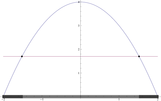
Figure 1: Figure 1: In the above figure, we see the s.c. (light gray) and p.p. (dark grey) spectra separated by the ”mobility edges” $\lambda^{\pm}=\pm 2\sqrt{(}1-\frac{v^{2}}{v_{c}})$, with $\frac{v}{v_{c}}=1,3038\cdots$.

Remark 1

The basic emphasis on one-dimensional (sparse) models has an important technical reason: the profound approach of Gilbert and Pearson connecting the space asymptotics of eigenfunctions of the restrictions of a large class of Sturm-Liouville operators to finite intervals to the spectral theory of these same operators in infinite space through the concept of subordinacy [GP87] is only available in one dimension. Using the important transfer matrix version of this theory due to Last and Simon [LS99], the surprise is that, even in a regime of strong sparsity, a spectral transition from s.c. to p.p. spectrum (first shown by Zlatos [Zla04]) may be proved: this is theorem 1. Our proof (theorem 4.7 of [MW12b]) differs from that in [Zla04] by the use of the (optimal) metrical version of Weyl’s theorem on uniform distribution [KN74] (in this case, of the so-called Prüfer angles, see [KLS98]) due to Davenport, Erdös and LeVeque [DEL63]. The latter permits an explicit characterization of the exceptional set in which the spectrum may not be of p.p. type (this exceptional set arises in connection with the concept of essential support of a measure [GP87]), which reveals it to be also of p.p. type. As a result, the spectrum at the edges of the band is proved to be purely p.p..

The robustness of the transition depicted in theorem 1 follows from [dRJLS96], because the Hausdorff dimension of the s.c. spectrum may be seen to be nonzero ([Zla04], [dCMW10]).

Finally, the difference Laplacean (2) leads to tunneling and bands [Fey65], with a pure a.c. spectrum. Starting from the difference Laplacean, the figure shows that any strength of the disorder $v$, however slight, yields p.p. spectrum in a nonempty range of energies. In addition, this occurs in a regime of strong sparsity. This is also true for the forthcoming models in $d\geq 2$ dimensions, and is thus a concrete manifestation of the tunneling instability, first studied by Jona-Lasinio, Martinelli and Scoppola [LMS81], and called by Simon a ”flea on the elephant” [Sim85], a phenomenon which has also dynamical counterparts [GS01], [WC98], and is at the root of the existence of the chiral superselection rules induced by the environment which account for the shape of molecules such as ammonia, see the review by A. S. Wightman [Wig95].

Unfortunately the s.c. spectrum does not posess either the dynamic or the perturbation theoretic properties (see [SW86], [How80]for the latter) which are commonly associated with the physical picture of delocalized states. Regarding the dynamical properties, for instance, the sojourn time of a particle with initial state $\Psi$ in a compact region $S$ is defined as

$$J(S;\Psi)\equiv\int_{-\infty}^{\infty}||P_{S}\exp(-itH)\Psi||^{2}dt$$

where $P_{S}$ denotes the projector on $S$. If $\Psi\in{\cal H}_{sc}$, it follows from a theorem by K.B. Sinha [Sin77] that a $S$ exists with $|S|<\infty$ and $J(S;\Psi)=\infty$. See also [MW12a], [MW12b] for further discussion.

We try therefore to attain higher dimensions.

Multidimensional version

Consider the Kronecker sum $J_{\phi}^{\omega}$ as an operator on $\mathcal{H}\otimes\mathcal{H}$:

$$J_{\theta}^{(2)}:=J_{\phi}^{\omega^{1}}\otimes I+\theta I\otimes J_{\phi}^{\omega^{2}}$$

$(6)$

where $\omega^{1}=\left(\omega_{j}^{1}\right)_{j\geq 1}$ and $\omega^{2}=\left(\omega_{j}^{2}\right)_{j\geq 1}$ are two independent sequences of independent random variables defined in $\left(\Omega,\mathcal{B},\nu\right)$, as before (we omit $\omega^{1}$ and $\omega^{2}$ in the l.h.s above for brevity). Above, the parameter $\theta\in[0,1]$ is included to avoid resonances . We ask for properties of $J_{\theta}^{(2)}$ (e.g. the spectral type) which hold for typical configurations, i.e., a.e. $\left(\omega^{1},\omega^{2},\theta\right)$ with respect to $\nu\times\nu\times l$ where $l$ is the Lebesgue measure in $[0,1]$. $J_{\theta}^{(2)}$ is a special two–dimensional analog of $J_{\phi}^{\omega}$; if the latter was replaced by $-\Delta+V$ on $L^{2}(\mathbb{R},dx)$ where $\Delta=d^{2}/dx^{2}$ is the second derivative operator, and $V$ a multiplicative operator $V\psi(x)=V(x)\psi(x)$ (potential), the sum above would correspond to $\left(-d^{2}/dx_{1}^{2}+V_{1}\right)+\left(-d^{2}/dx_{2}^{2}+V_{2}\right)$ on $L^{2}(\mathbb{R}^{2},dx_{1}dx_{2})$, i.e., the ”separable case” in two dimensions. Accordingly, we shall also refer to $J_{\theta}^{(n)}$, $n=2,3,\ldots$, as the separable case in $n$ dimensions.

Our approach was to look at the quantity

$$\left(\Phi,e^{-itJ_{\theta}^{(2)}}\Psi\right)=f^{1}(t)f^{2}(\theta t)$$

where

$$f^{i}(s)=f_{\mathrm{sc}}^{i}(s)+f_{\mathrm{pp}}^{i}(s)~{},\quad i=1,2$$

$$\mbox{ with }f_{\mathrm{sc}}^{i}(s) = \int e^{-is\lambda}d\mu_{\varphi_{i},\psi_{i}}^{\mathrm{sc}}(\lambda)$$

$$f_{\mathrm{pp}}^{i}(s) = \int e^{-is\lambda}d\mu_{\rho_{i},\chi_{i}}^{\mathrm{pp}}(\lambda)$$

Above $\Phi,\Psi\in\mathcal{H}\otimes\mathcal{H}$,

$$\Phi = \left(\varphi_{1}\dot{+}\rho_{1}\right)\otimes\left(\varphi_{2}\dot{+}\rho_{2}\right)~{},$$

$$\Psi = \left(\psi_{1}\dot{+}\chi_{1}\right)\otimes\left(\psi_{2}\dot{+}\chi_{2}\right)~{},$$

with $\varphi_{i},\psi_{i}\in\mathcal{H}_{\mathrm{sc}}$, $\rho_{i},\chi_{i}\in\mathcal{H}_{\mathrm{pp}}$ and $\varphi\dot{+}\rho$ denotes the direct sum of two vectors $\varphi,\rho\in\mathcal{H}$.

We shall use the following folklore proposition (see, e.g., theorem 3.2 of [MW12b] or [Sin77]):

Proposition 1

Let $\mu$ be a measure on the space $M(\mathbb{R})$ of all finite regular Borel measures on $\mathbb{R}$. If the Fourier–Stieltjes transform of $\mu$

$$\mathbb{R}\ni t\longmapsto\hat{\mu}(t)=\int e^{-it\lambda}d\mu(\lambda)$$

belongs to $L^{2}(\mathbb{R},dt)$, then $\mu$ is absolutely continuous with respect to Lebesgue measure.

The time-like decay of the Fourier-Stieltjes (F.S.) transform of the spectral measure is dictated by the Hausdorff dimension of the spectral measure:

Let $S$ be a subset of $\mathbf{R}$, $\alpha\in[0,1]$, and $\delta>0$. Define

$$h^{\alpha}_{\delta}(S)\equiv\inf\{\sum_{j=1}^{\infty}|C_{j}|^{\alpha}$$

$$|S\subset\cup_{j=1}^{\infty}C_{j}\mbox{ with }|C_{j}|\leq\delta\}$$

where $|C|$ denotes the Lebesgue measure (length) of $C$, and

$$h^{\alpha}(S)=\lim_{\delta\to 0}h^{\alpha}_{\delta}(S)=\sup_{\delta>0}h^{\alpha}_{\delta}(S)$$

We call $h^{\alpha}$ $\alpha$ - dimensional Hausdorff measure on $\mathbf{R}$. $h^{1}$ agrees with Lebesgue measure, and $h^{0}$ is the counting measure, so that $\{h^{\alpha}|0\leq\alpha\leq 1\}$ is a family which interpolates continuously between the counting measure and Lebesgue measure.

Definition 1 A Borel measure on $\mathbf{R}$ is uniformly alpha-Hoelder continuous (U$\alpha$H) if there exists $C$ such that for every interval $I$ with $|I|<1$,

$$\mu(I)<C|I|^{\alpha}$$

By an important theorem of Last [Las96], U$\alpha$H measures may be obtained by a process of closure. In our one-dimensional model the Hausdorff dimension varies locally in the s.c. spectrum, and the local Hausdorff dimension (suitably defined) may be determined explicitly. There exists a dense set in the s.c. subspace such that the spectral corresponding spectral measure is U$\alpha$H. We shall for simplicity assume that the Hausdorff dimension has a constant value which will be denoted by $\alpha$.

The basic theorem, due to Strichartz [Str90] (with a very slick alternative proof by Last [Las96], therefore we call it Strichartz-Last theorem), relates decay in the Cesaro sense to the Hausdorff dimension:

Strichartz-Last theorem

Let $\mu$ be a finite U$\alpha$H measure and, for each $f\in L^{2}(\mathbf{R},d\mu)$, denote

$$\hat{f\mu}(t)\equiv\int\exp(-ixt)f(x)d\mu(x)$$

Then there exists $C$ depending only on $\mu$ such that for all $f\in L^{2}(\mathbf{R},d\mu)$ and $T>0$,

$$\langle|\hat{f\mu}|^{2}\rangle_{T}<C||f||^{2}T^{-\alpha}$$

where $||f||$ denotes the $L^{2}$ - norm of $f$, and $\langle g\rangle_{T}\equiv\frac{\int_{0}^{T}g(t)dt}{T}$.

A measure is called a Rajchman measure iff

$$\lim_{|t|\to\infty}\hat{\mu}(t)=0$$

It does not follow from the decay in the Strichartz-Last theorem that the corresponding measure is Rajchman . Let $E$ denote the usual Cantor ”middle-thirds” set in $[-\pi,\pi]$; die F.S. transform of the corresponding measure $\Gamma$ is:

$$\Gamma(u)=\prod_{j=1}^{\infty}\cos[2/3u\pi 3^{-j+1}]$$

The corresponding Hausdorff dimension is well-known to be $\alpha=\frac{|\log 1/2|}{|\log 1/3|}$ und the measure is U$\alpha$H, but, from the above formula for $\Gamma$ it follows that

$$\Gamma(n)=\Gamma(3n)\mbox{ for all }n\in\mathbf{Z}$$

and hence the Cantor measure is not Rajchman.

The main result of [MW12a] was:

Theorem 2 Let

$$v^{2}<a\left(\sqrt{\beta}-1\right)<v_{c}^{2}$$

with $a<4$, where $v_{c}=2\sqrt{(}\beta-1)$. Then, for almost every $\left(\omega^{1},\omega^{2},\theta\right)$ with respect to $\nu\times\nu\times l$, [a.] there exist $\tilde{\lambda}^{\pm}$ with $\tilde{\lambda}^{+}=-\tilde{\lambda}^{-}$ and

$$0<\tilde{\lambda}^{+}<\lambda^{+}$$

such that

$$\left(\tilde{\lambda}^{-}(1+\theta),\tilde{\lambda}^{+}(1+\theta)\right)\subset\sigma_{\mathrm{ac}}\left(J_{\theta}^{(2)}\right)$$

[b.]

$$\left[-2(1+\theta),\lambda^{-}(1+\theta)\right)\cup\left(\lambda^{+}(1+\theta),2(1+\theta)\right]\subset\sigma_{\mathrm{pp}}\left(J_{\theta}^{(2)}\right)$$

[c.]

$$\sigma_{\mathrm{sc}}\left(J_{\theta}^{(2)}\right)\cap\left(\lambda^{-}(1+\theta),\lambda^{+}(1+\theta)\right)$$

may, or may not, be an empty set.

The basic idea of the proof is that the Strichartz-Last theorem suggests a pointwise decay of the F.S. transform of the spectral measure of type $t^{-\alpha/2}$ for large $t$. For the Kronecker sum (with $\theta=1$) the F.S. transform is the product of the corresponding transforms for the one-dimensional system, which we expect decays as $t^{-\alpha}$. In order to use the proposition, we restrict the spectral measure to an interval in the s.c. spectrum such that $2\alpha>1$ which is in principle non-empty (and may be proven so), and denote the F.S. transform of the thus restricted measure by the same symbol as before. It turns, however, out that this heuristics is not correct mathematically: as shown above, Cesaro decay does not in general imply pointwise decay or, in other words, that the spectral measure is Rajchman. This is a much harder problem - (see [MW12b], chapter 4 for the full treatment of the pointwise decay of a model with superexponential sparsity and pure s.c. spectrum, and the recent very hard analysis to prove local decay in nonrelativistic QED [TJFS12]). Moreover, the result for general $\theta$ may not be true due to resonance between Cantor sets, a subtle phenomenon which has been so far analysed only in the self-similar case by Hu and S.G. Taylor [HT94]. Self-similarity occurs, however, seldom: indeed, the s.c. spectrum of sparse Jacobi matrices is not self-similar by a theorem of Combes and Mantica [CM01]. We proved, however, that the main idea is indeed correct by generalizing a method due to Kahane and Salem ([KS94], [KS58]) in specific (self-similar) cases to the problem at hand.

We shall come back to this model in section 2d.

2b2 - Anderson model on the Bethe lattice

Consider a particle moving - for simplicity - on the Bethe lattice, a regular rooted tree graph, with vertex set ${\cal G}$, in which each vertex, aside from the root $O$ has $K+1$ neighbors with $K\geq 2$, and an edge set ${\cal E}$, described by a Schrödinger operator of the form

$$(H_{\lambda}(\omega)\Psi)(x)=-\sum_{(x,y)\in{\cal E}}\Psi(y)+\lambda V^{\omega}(x)\Psi(x)$$

$V^{\omega}$ is a real valued random potential, with $\omega$ again representing the randomness. We assume, again for simplicity, that the $\{V^{\omega}(x)\}_{x\in{\cal G}}$ comprise i.i.d. random variables, whose probability distribution is of the form $\rho(V)dV$ with $\rho$ the uniform distribution, constant over the interval $[-1,1]$ and zero elsewhere (the uniform distribution). The regularity conditions assumed in [AW11b], [AWb], [AWa] are much more general, but the uniform distribution is always a possible special case, and is the simplest example to be kept in mind. $H_{\lambda}(\omega)$ is a bounded self-adjoint operator on $l^{2}({\cal G})$, with spectrum which is, for almost all realizations of $\omega$, the nonrandom set

$$\sigma(H_{\lambda})=[-|E_{\lambda}|,|E_{\lambda}|]\mbox{ with }E_{\lambda}=-(2\sqrt{(}K)+\lambda)$$

The fact that the spectral measures associated to the different vectors $\delta_{x}\in l^{2}({calG})$, where $\delta_{x}$ denotes the Kronecker delta at $x$, are almost surely all equivalent, i.e., a.s. cyclicity of the spectrum, is an important result of [Jl00].

For a tree with $N$ generations, there are $N_{S}=(K+1)K^{N-1}$ vertices at the surface (generation $N=0$) and a total $N_{T}=(K^{N+1}+K^{N-2})/(K-1)$ vertices. Since the ratio $N_{S}/N_{T}$ is nonzero for $N\to\infty$, the behavior of statistical systems on a Bethe lattice is quite distinct from those on a regular Bravais lattice.

Models such as (7) have been considered since the early days of Anderson localization, see [And58],[RACT73], [ACT74]. The first mathematical proof of a transition was the seminal result of A. Klein [Kle98]:

Theorem 3 (Theorem 1.1 of [Kle98]) For any $E$, $0<E<2\sqrt{(}K)$, there exists $\lambda(E)>0$ such that for any $\lambda$ with $|\lambda|<\lambda(E)$ the spectrum of $H_{\lambda}$ in $[-E,E]$ is purely a.c. with probability one.

Aizenman [Aiz94] proved localization in the Bethe lattice for energies beyond $K+1$, at weak disorder: this quantity appears as the edge of the $l^{1}$- spectrum of the free Laplacean on the lattice. What happens between $2\sqrt{(}K)$ and $K+1$ for small $\lambda$? (This is problem 4 in Jitomirskaya’s list of open problems). As noted in [Jit07], bottom of page 626, in analogy with the random surface case or the random decaying potentials mentioned in section 2a, one might conjecture that $l^{1}$- phenomena prevail up to the $l^{2}$- threshold, i.e., that there is localization up to near the edge of the $l^{2}$ spectrum - but see the following theorem 4b, due to [AW11b], [AWb], a surprising result which contradicted original expectations, and whose ideas we now briefly sketch.

As explained in [AW11a], [AW11b], and stated heuristically, states which may locally appear to be localized have arbitrarily close energy gaps $\Delta E$ with other states to which the tunneing amplitudes decay exponentially in the distance $R$, as $\exp(-L_{\lambda}(E)R)$, where $L_{\lambda}(E)$ is the Lyapunov exponent defined as follows. Let

$$G_{\lambda}(x,y;\zeta,\omega)=(\delta_{x},(H_{\lambda}(\omega)-\zeta)^{-1}\delta_{y}))$$

where $\zeta\in\mathbf{C}^{+}\equiv\zeta\in\mathbf{C}\mbox{ s.t. }\Im\zeta>0$ denote the Green’s function. Then

$$L_{\lambda}(E)\equiv-\lim_{\eta\searrow 0}Av(|\log|G_{\lambda}(0,0;E+i\eta,\omega)|)$$

where $Av$ stands for the expectation over the $\omega$ probability distribution. Indeed, it is shown in [AWb] that on tree graphs $L_{\lambda}$ provide the typical decay rate of the Green’s function:

$$\lim_{\eta\searrow 0}G_{\lambda}(0,x;E+i\eta,\omega)\sim C\exp(-L_{\lambda}(E)|x|)$$

a.s. in $\omega$, where the limit exists for a.e. energy $E$ and $|x|=d(x,0)$ denotes the graph distance of the vertex $x$ to some fixed but arbitrary vertex $O\in{\cal G}$. Mixing between two levels would occur if $\Delta E\ll\exp(-L_{\lambda(E)}R)$, which is a very stringent condition, not satisfied in finite dimension, but, since, as previously remarked, the volume grows exponentially, as $K^{R}=\exp(R\log K)$, extended states may form, and a sufficient condition may be shown to be $L_{\lambda}(E)>\log K$:

Theorem 4a (Theorem 1 of [AW11b], see also [AWb] Under the previous assumptions, at a.e. $E\in\sigma(H_{\lambda})$ at which also

$$L_{\lambda}(E)>\log K$$

one has, with probability one,

$$\Im G_{\lambda}(x,x;E+i0,\omega)>0$$

for all $x\in{\cal G}$.

Above, $E+i0$ denotes $\lim_{\eta\searrow 0}$ of the corresponding quantity with argument $E+i\eta$. It is well known that

$$\pi^{-1}\Im G_{\lambda}(x,x;E+i0,\omega)$$

is the density of the a.c. component of the spectral measure associated with the state $|x>\equiv\delta_{x}$ (see, e.g., [Jak06], Theorem 3.15), and thus theorem 4a implies that in any energy interval within $\sigma(H_{\lambda}(\omega))$ for which (10a) holds, the random operator a.s. has some a.c. spectrum on a subset of energies of positive Lebesgue measure. We now have:

Theorem 4b (Theorem 2 of [AW11b]) For

$$\lambda<\Delta_{K}\equiv(\sqrt{(}K)-1)^{2}/2$$

condition (10-a) holds for all energies satisfying

$$|E|>|E_{\lambda}|-\delta(\lambda)$$

at some $\delta(\lambda)>0$.

Clearly (10-e) includes the spectral edges $[E_{\lambda},E_{\lambda}+\delta(\lambda))\cup(|E_{\lambda}|-\delta(\lambda),|E_{\lambda}|]$. Thus, for $\lambda$ small enough (as in theorem 4b), near the spectrum’s boundary the random operator has a.s. only purely a.c. spectrum, and thus there is no mobility edge beyond which the spectrum is pure point and localization sets in - a surprising result, which contradicts original expectations [RACT73][ACT74]. On the basis of the joint continuity of $L_{\lambda}(E)$ in $(\lambda,E)$, it has also been conjectured [AW11b] that for small enough $\lambda$ - for bounded potentials and sufficiently regular probability distributions - the spectrum is purely a.c..

An improved version of theorem 4a includes information about large deviations, which are encoded in the free energy function, defined for $s\in[-\kappa,1)$ - where $\kappa\in(0,1)$ is such that $Av(V(0)^{\kappa})<\infty$ - by

$$\phi_{\lambda}(s;E)\equiv\lim_{|x|\to\infty}\frac{\log Av(|G_{\lambda}(0,x;E+i0,\omega)|^{s})}{|x|}$$

and for $s=1$ by $\phi_{\lambda}(1;E)\equiv\lim_{s\nearrow 1}\phi_{\lambda}(s;E)$. The existence of the limit in (11-a), for a.e. $E\in\mathbf{R}$, is shown in ([AWb], Theorem 3.2). We have

Theorem 4c (Theorem 2.5 of [AWb]) Under the previous assumptions (but, much more generally, assumptions A-E, pg.8, of [AWb]), for any $\lambda>0$ and Lebesgue a.e. $E\in\mathbf{R}$ at which

$$\phi_{\lambda}(1;E)<-\log K$$

the Green’s function satisfies almost surely

$$\Im G_{\lambda}(0,0;E+i0,\omega)>0$$

By convexity arguments (see, again, theorem 3.2 of [AWb]), $\phi_{\lambda}(s;E)\geq-sL_{\lambda}(E)$, and, hence, (11-b) implies (10-a) and, therefore, Theorem 4a is satisfied under the assumption of theorem 4a.

The importance of the free energy function is two-fold: it characterizes almost completely the different spectral regimes (see [AWb]), and it is also a powerful tool in the dynamics, a topic to which we now turn our attention.

2c - Dynamics

We have seen the importance of the dynamics for spectral theory already in section 2a, through quantities like the sojourn time (5) and the idea of the proof of theorem 2. This is also true regarding theorem 3, which makes use of the fact that the FS transform of the spectral measure (associated to the Kronecker vector $\delta_{0}$ for instance), defined as in proposition 1, satisfies

$$\int_{-\infty}^{\infty}|\hat{\mu}(t)|^{2}dt$$

$$\leq\frac{1}{\pi}\liminf_{\eta\rightarrow 0+}\int_{-\infty}^{\infty}|G_{\lambda}(0,0;E+i\eta,\omega)|^{2}dE$$

by the Plancherel theorem and Fatou’s lemma (see [Kle98] or exercise 3.5 of [MW12b]). Klein succeeded in proving that

$$\liminf_{\eta\searrow 0}\int_{-E}^{E}|G_{\lambda}(x,x;E^{{}^{\prime}}+i\eta,\omega)|^{2}dE^{{}^{\prime}}<\infty$$

with probability one for certain values of $(E,\lambda)$ mentioned in the statement of theorem 3, from which the spectral measure restricted to $(-E,E)$ is purely a.c. by proposition 1.

Another interesting dynamical consequence of (11-c) was emphasized by Miller and Derrida [MD94], in a basic theoretical paper on weak disorder expansions: if quantum particles are sent coherently at energy $E=k^{2}+U_{\mbox{ wire }}$ down a wire attached to the graph at the vertex $x$, the reflection coefficient $R_{E}$ satisfies $R_{E}<1$ iff (11-c) holds, see also the discussion in [AW11b], pg.3.

A different class of problems involving the dynamics relates to quantum dynamical stability. We briefly summarize the main issues, following ([MW12b], section 3d). Most of the concepts of dynamical stability in quantum mechanics are related to the growth of expectation values

$$\langle A(t)\rangle$$

of certain observables $A=A(0)$ as time $t$ evolves. Boundedness of $\langle A(t)\rangle$ is related to quantum stability. In general, for a lattice model such as the the Anderson model if the potential is random, or the case of an almost-periodic potential, it is common to adopt $A=|X|^{2}$, where $X$ denotes the operator of multiplication by the coordinate $X$, and one distinguishes the localization regime in which $\langle|X|^{2}\rangle<C$ for all $t$, or the ballistic regime where

$$\langle|X|^{2}\rangle=O(t^{2})\ ,\qquad\text{as }t\rightarrow\infty$$

which are supposed to correspond, respectively, to p.p. and a.c. spectrum; Intermediate regimes are characterized by the diffusion constant

$$D_{\Psi}=\lim_{t\rightarrow\infty}\frac{\langle|X|^{2}\rangle}{t}$$

when the above limit exists , and the dependence on the initial state $\Psi$ is explicitly indicated.

If $\langle|X|^{2}\rangle<C$ with $C$ a positive constant for all $t$, then $\Psi$ has no continuous component. This is corollary 2.3.1. of [Las96], and implies that $D_{\Psi}=0$. It is remarkable that the converse, i.e., that if $\Psi\in\mathcal{H}_{\mathrm{pp}}$, then $D_{\Psi}=0$, is not true. Indeed, the only general result about the converse is Simon’s paper [Sim90] on the absence of ballistic motion, i.e., $\lim_{t\rightarrow\infty}\langle|X|^{2}(t)\rangle=0$ if $\Psi\in\mathcal{H}_{pp}$, which is far from the expected $D_{\Psi}=0$. The reason for this is the instability of the two exotic spectra, dense p.p. and s.c.; indeed, even a rank one perturbation with arbitrarily small norm is able to induce a transition from one type to the other! ([How92, SW86]). Since one does not expect the dynamics to be strongly affected by such perturbations, it is plausible that the absence of ballistic motion - the latter characterizing a.c. spectra - is both a feature of s.c. spectra and the (thick) p.p. spectra obtained from s.c. spectra by such perturbations: therefore Simon’s result might be optimal! This has indeed be shown in the remarkable paper [dRJLS96], where a potential was constructed such that the Hamiltonian $H$ on $l^{2}(\mathbb{Z})$ has a complete set of exponentially decaying eigenfunctions but, for any $\delta>0$, $||X\exp(-itH)\delta_{0}||^{2}/t^{2-\delta}$ is unbounded as $t\rightarrow\pm\infty$. Note that $||x\exp(-itH)\delta_{0}||^{2}=(\exp(-itH)\delta_{0},X^{2}\exp(-itH)\delta_{0})$. In the words of Jitomirskaya [Jit07], this example showed that mere “exponential localization” of eigenfunctions need not have any consequence for the dynamics. Thus, [dRJLS96] was pioneer in demonstrating the importance of dynamical localization , which, since then, was proved for various random models in the form

$$\sup_{t}\left\|\left|X\right|^{q}E_{I}(H_{\omega})\exp(-itH_{\omega}\Psi)\right\|<\infty$$

with probability one. $I\subset\mathbb{R}$ is an energy interval in the localization region and $E_{I}$ are spectral projections for $I$. For the Anderson Hamiltonian, or the deterministic almost-Mathieu model, several results are known, and we refer to ([Jit07], p. 621) for a discussion and (numerous) references.

Concerning now the diffusion constant $D_{\Psi}$ given by (12-b), one may define the so-called diffusion exponents (see, e.g., [BSB00]):

$$\beta_{m}^{\pm}(\Psi)=\lim_{\pm}\frac{\log\langle|X|^{m}\rangle_{T}}{\log(T^{m})}$$

where $\lim_{\pm}\equiv\limsup_{T\to\infty}(\liminf_{T\to\infty})$. Both $\beta_{m}^{\pm}(\Psi)$ are nonincreasing functions of $m$ and obey

$$0\leq\beta_{m}^{-}(\Psi)\leq\beta_{m}^{+}(\Psi)\leq 1$$

$(12-d)$

The following important theorem ([Gua89], [Las96], [Com93]) relates the above quantities to the Hausdorff dimension of the s.c. spectrum:

Guarneri-Last-Combes (GLC) theorem If $H$ is self-adjoint on $\mathcal{H}$ with spectral family $\{E(\lambda\}$ and uniformly alpha Hoelder continuous spectral measure $\mu_{\Psi}(\lambda)=(\Psi,E(\lambda)\Psi)$ (definition 1) there exists a constant $c_{\Psi,m}$ depending on $\Psi$ and $m$ such that, for all $T>0$ and $m>0$,

$$\langle(\Psi(t),|X|^{m}\Psi(t))\rangle_{T}>c_{\Psi,m}T^{m\alpha/d}$$

Above, the time average $<.>_{T}$ is defined as in the statement of the Strichartz-Last theorem. By the GLC theorem,

$$\beta_{m}^{-}(\Psi)\geq\alpha/d$$

For $\mu_{\Psi}$ a.c., $\alpha=1$; hence, in dimension $d=1$, a.c. spectrum implies ballistic transport, while in dimension $d=3$, a.c. spectrum and subdiffusive motion ($\beta_{m}<1/2$) may coexist. This motion is experimentally found in the so-called quasicrystals (see [GSB99] for a discussion and references). One of the very few models in $d=3$ dimensions exhibiting a.c. spectrum with subdiffusive motion this was constructed in [BSB00] along lines similar to those of theorem 2, but using one-dimensional Jacobi matrices with self-similar s.c. spectra and making use of the aforementioned theorem of Hu and Taylor [HT94].

Defining the transition probability

$$P_{\Psi,t}(x)\equiv|(\exp(-itH)\Psi)(x)|^{2}$$

a different form of the time-average (for the observable $|x><x|$) is often easier to study [AWa]:

$$\hat{P}_{\Psi,\eta}(x)\equiv 2\eta\int_{0}^{\infty}\exp(-2\eta t)P_{\Psi,t}(x)dt$$

$$=\frac{\eta}{\pi}\int|((H-E-i\eta)^{-1}\Psi)(x)|^{2}dE$$

$(13-b)$

with inverse time parameter $\eta>0$ playing the role of $1/T$ in the aforementioned time-averages: the limit of long time averages $T\to\infty$ becomes $\eta\searrow 0$. The equality (13-b) follows from the spectral theorem and Plancherel’s theorem and explains the utility of this type of averaging. The averages (12-a) may now be written, with $A(0)=|X|^{\beta}$,

$$M_{\Psi}(\beta,t)=\sum_{x\in{\cal G}}|x|^{\beta}P_{\Psi,t}(x)$$

and the modified time-averages as

$$\hat{M}_{\Psi}(\beta,\eta)\equiv\sum_{x\in{\cal G}}|x|^{\beta}\hat{P}_{\Psi,\eta}(x)$$

Ballistic (resp. diffusive) transport (12b)(resp. (12c)) correspond to $r=1$ (resp. $r=1/2$) in the formulas:

$$M_{\Psi}(\beta,t)\sim t^{r\beta}$$

and

$$\hat{M}_{\Psi}(\beta,\eta)\sim\eta^{-r\beta}$$

in the finite-dimensional case ${\cal G}=\mathbf{Z}^{d}$.

A general ballistic upper bound

$$\hat{M}_{\Psi}(\beta,\eta)\leq C(\beta,\Psi)\eta^{-\beta}$$

for all normalized $\Psi\in l^{2}({\cal G})$ with $\sum_{x\in{\cal G}}|x|^{\beta}|\Psi(x)|^{2}<\infty$, follows from general arguments related to the Lieb-Robinson bounds [NS06], see the appendix B of [AWa].

The strategy of proving the lower bound of the same type of the r.h.s. of (14-c) (with the purpose of showing ballistic behavior) is of particular interest. By the GLC theorem, for ${\cal G}=\mathbf{Z}^{d}$, in the case of uniformly alpha Hoelder continuous spectral measures, the Guarneri bound (see also [Gua89]) becomes

$$\hat{P}_{\Psi,\eta}(x)\leq C\eta^{\alpha}$$

, and thus

$$\hat{Pr}_{\Psi,\eta}(|x|<b\eta^{-\alpha/d})\equiv\sum_{|x|<b\eta^{-\alpha/d}}\hat{P}_{\Psi,\eta}(x,t)$$

$$<C_{d}b^{d}$$

$(15-b)$

which implies that (14-a,b) can only hold if $r\geq\alpha/d$, because, selecting $b$ such that $C_{d}b^{d}=1/2$ one obtains $\hat{M}_{\Psi}(\beta,\eta)\geq\frac{b^{\beta}\eta^{-\beta\alpha/d}}{2}$. This lower bound diminishes, however, as $d\to\infty$, and provides no information in this limit (which is the tree graph case). A different method becomes, therefore, necessary, of which we sketch the main ideas. With the notion of a.c. spectrum defined by

$$\sigma_{ac}(H)\equiv\{E\in\mathbf{R}|Pr(\Im G(0,0;E+i0)\neq 0)>0\}$$

where $Pr$ denotes the probability associated to the random potential (we refer to [AWa] for further discussion of this concept, but remark that $\sigma_{ac}(H)$ is a nonrandom set which is a.s. the support of the a.c. component of the spectrum), the following theorem holds:

Theorem 5 (Theorem I.1 of [AWa]) For any initial state of the form $\Psi=f(H)\delta_{0}$, with a measurable function $f\in L^{2}(\mathbf{R})$ supported in $\sigma_{ac}(H)$, and all $b>0$,

$$Av(\hat{Pr}_{\Psi,\eta}(|x|<b\eta^{-1})\leq C(f)b+o(\eta)$$

with some $C(f)<\infty$ and $o(\eta)$ a quantity which vanishes for $\eta\to 0$.

Theorem 5 yields a lower bound to $\hat{M}_{\Psi}(\beta,\eta)$ of the ballistic form r.h.s. of (14-c); together with (14-c) it implies ballistic behavior for the full regime of the a.c. spectrum. Its significance is due to the following facts: i.) in the hyperbolic geometry of a regular tree, the classical diffusion (which corresponds to $r=1/2$ in (14) in the finite dimensional case) also spreads ballistically, since, at each instant, there are more directions at which $|x|$ would increase than the one direction at which it goes down ; ii.) it excludes the possibility of a different behavior in the previously discussed regime where the a.c. spectrum is caused by rare resonances, such as around the edges, where the density of states is very low and Lifschitz tail asymptotics hold (see [AW11a]).

The following diffusive bound is (for a bounded measurable $I\subset\sigma_{ac}(H)$) the main ingredient of the proof of theorem 5:

$$esssup_{\zeta\in I+i(0,1]}Av(|G(0,x;\zeta)|^{2})\leq\frac{C(I)}{K^{|x|}}$$

where $C(I)<\infty$. The r.h.s. of (16a) coincides with the mean value of the total time spent at vertex $x$ for a particle undergoing diffusion at the root $x=0$. This bound is a consequence of the following bounds for the free energy function (11a):

$$\phi(s;\zeta)\leq-s\log K\mbox{ for all }\zeta\in\mathbf{C}^{+}$$

$$\mbox{ and for all }s\in[0,2]$$

$(16-b)$

and

$$Av(|G(0,x;\zeta)|^{s}\leq C_{+}(s,\zeta)\exp[\phi(s;\zeta)|x|]$$

$$\mbox{ for all }s\in[0,1)\mbox{ and }x\in{\cal G}$$

$(16-c)$

where $C_{+}(s,\zeta)\in(0,\infty)$ uniformly in $\zeta\in[-E,E]+i(0,1]$ for any $0\leq E<\infty$ at a fixed $s\in[0,1)$.

Since for energies in the p.p. spectrum $Av(|G(0,x;E+i0)|)=\infty$ (see, e.g., [Jak06], theorem 3.15), (16c) cannot be expected to hold beyond $s=1$, but theorem II.2 of [AWa] shows that this bound extends to all energies such that

$$esssup_{\zeta\in I+i90,1]}Av((\Im G(0,0;\zeta))^{-3-\delta})<\infty$$

for some $\delta>0$, and then theorem II.4 of [AWa] shows that (16-d) includes any bounded measurable set $I\subset\sigma_{ac}(H)$, with $\sigma_{ac}(H)$ given by (15-c).

2d - Concluding remarks on the Anderson transition

An essential point, noted in [Jit07], is that Klein’s proof of theorem 3 uses the looples character of the graph in an essential way and, thus, the Bethe lattice, while corresponding to the limit $d\to\infty$, is, in a sense, one-dimensional. Similarly, the sparse model of section 2b1 also has no loops, because theorem 2 ”inherits” the one-dimensional structure of the model of theorem 1. Thus, both models still run short of solving the central issues of the original model, which remains one of the basic challenges of mathematical physics.

The model on the Bethe lattice describes the limit $d\to\infty$ and, as remarked in [AW11b], the new and surprising phenomena found there may even have wider applicability due to the analogies drawn between tree graphs and many-particle configurations [BAL97]. They are, however, not expected in finite dimensions, in particular the absence of the mobility edge for weak disorder (Theorem 4b) is not found in the sparse model (see theorem 1 and theorem 2, where the existence of p.p. spectrum in a nonempty energy interval for arbitrarily small disorder is pictured as a concrete example of the tunneling instability). However, the methods used to prove theorem 4b, in particular concerning the free energy function (11a), may have wider applicability, in particular to investigate the existence or not of a sharp mobility edge in other models, such as the one in section 2b1 or Krishna’s model [Kric]. In addition, the ideas developed for the Bethe lattice dynamics reviewed in 2c, such as related to the negative moments of the Green’s function (16-d), also deserve special attention as potentially powerful methods to prove existence of the a.c. spectrum.

On the other hand, sparse models such as the one depicted in section 2b1, in dimension $d\geq 2$, comprise a part of the full model on a Bravais lattice. Although exponential sparsity is too severe, it should be recalled that the separable model (6) does not take account of dimensionality in a proper way, because in ”truly d-dimensional” sparse models the cardinality of the set in (4) may change from $O(\log R)$ to $O(R^{d-\epsilon})$, for some $\epsilon>0$, and ”filling in” the remaining points may be expected to remedy this flaw, but this is an immensely challenging open problem! The sparse version has, however, one promising feature as compared with the full Anderson model: in the latter, the $d\geq 2$ version built as in (6) from the one-dimensional version (the separable full Anderson model) continues to have purely p.p. spectrum, by [GMP77] and the fact that convolutions of p.p. measures are p.p., in complete disagreement with the expected transition. It may thus seem worthwhile to study sparse models such as that of 2b1 as prospective descriptions of lightly doped semiconductors, which are also expected to exhibit an Anderson transition in dimension $d\geq 2$ [SE84]. Of course, non-sparse models such as the one proposed in [Kric], are also very promising, although the available picture of the transition seems to be, as yet, somewhat less detailed than the model described in section 2b1.

3-Frustration and short-range spin glasses: the Edwards-Anderson model

Dilute solutions of atoms of large magnetic moments (such as the transition metals Fe, Co, Mn) in a paramagnetic substrate (Cu, Au) present a number of peculiar physical properties. For small, but sufficiently high concentrations of magnetic impurities, the susceptibility in low fields displays a characteristic peak, with discontinuous derivatives, at a temperature $T_{g}$. The specific heat is always smooth, with a linear dependence on the temperature as $T\to 0$. The behaviour of these spin glasses has been explained in terms of an indirect RKKY interaction between the spins of these magnetic impurities mediated by the electrons of the paramegnetic matrix [BY86], which is of the form $-J(|i-j|)S_{i}S_{j}$ with $J(r)=(k_{F}r)^{-3}\cos(2k_{F}r)$, where $r$ is the distance between magnetic atoms and $k_{F}$ the fermi momentum; $S_{i}=\pm 1$ are (e.g.) Ising spins. The rapid oscillations and the weak decay of $J(r)$, as well as the random distribution of the impurity magnetic atoms, are the basic ingredients of spin glasses. At sufficiently low temperatures there is a ”freezing” of the magnetic moments in random directions (which leads to an increase of the susceptibility). The spin glass phase may be regarded as a conglomerate of blocks of spins, each block with its own characteristic orientation, in such a way that there is no macroscopic magnetic moment [BY86].

Edwards and Anderson [EA75] proposed a spin Hamiltonian, which we write in a generalized version as follows. For each finite set of points $\Lambda\subset\mathbf{Z}^{d}$, where the dimension $d$ will be restricted to the values $d=2$ and $d=3$, consider the Hamiltonian

$$H_{\Lambda}(\{J\})=\sum_{i,j\in\Lambda}J_{i,j}\Phi_{i,j}$$

where $\Phi_{i,j}$ with $i,j\in\Lambda$ are self-adjoint elements of the algebra generated by the set of spin operators, the Pauli matrices $\sigma_{i}^{x}$, $\sigma_{i}^{y}$, $\sigma_{i}^{z}$, $i\in\Lambda$, on the Hilbert space ${\cal H}_{\Lambda}=\otimes_{i\in\Lambda}\mathbf{C}_{i}^{2}$, given by

$$\Phi_{i,j}=\alpha_{x}\sigma_{i}^{x}\sigma_{j}^{x}+\alpha_{y}\sigma_{i}^{y}\sigma_{j}^{y}+\alpha_{z}\sigma_{i}^{z}\sigma_{j}^{z}$$

for $|i-j|=1$, and zero otherwise. The random couplings $J_{i,j}$, with $|i-j|=1$, are random variables (r.v.) on a probability space $(\Omega,{\cal F},P)$, where ${\cal F}$ is a sigma algebra on $\Omega$ and $P$ is a probability measure on $(\Omega,{\cal F})$. We may take without loss of generality

$$\Omega=\times_{B^{d}}S$$

where $S$ is a Borel subset of $\mathbf{R}$, $B^{d}$ is the set of bonds in $d$ dimensions, and assume that the $J_{i,j}$ are independent, identically distributed r.v.. In this case, $P$ is the product measure

$$dP=\times_{B^{d}}dP_{0}$$

of the common distribution $P_{0}$ of the random variables, which will be denoted collectively by $J$. The corresponding expectation (integral with respect to $P$) will be denoted by the symbol $Av$. We have to assume that

$$Av(J_{i,j})=0$$

for all $i,j\in\mathbf{Z}^{d}$, i.e., that the couplings are centered. This assumption mimicks the rapid oscillations of the RKKY interaction. Let $E_{\Lambda}$ denote the GS energy of $H_{\Lambda}$, i.e., $E_{\Lambda}=\inf spec(H_{\Lambda})$. The following result was proved, among several others, in [CL10]:

Theorem 6 ([CL10]) For $P$- a.e. $\{J\}$, the limit below exists and is independent of the b.c.:

$$e^{(d)}\equiv\lim_{\Lambda\nearrow\mathbf{Z}^{d}}\frac{E_{\Lambda}}{|\Lambda|}$$

and

$$e^{(d)}=\inf_{\Lambda}\frac{E_{\Lambda}}{|\Lambda|}$$

where $|\Lambda|$ denotes the number of sites in $\Lambda$. Finally,

$$e^{(d)}\geq e^{(d+1)}$$

(21-a) is the far-reaching property of self-averaging (see [And78] for a discussion): it expresses that measurable - e.g. thermodynamic- quantities are the same for any typical configuration of the sample, i.e., are experimentally reproducible. It follows from (21a) that, $P$- a.e.,

$$e^{(d)}=\lim_{\Lambda\nearrow\mathbf{Z}^{d}}\frac{Av(E_{\Lambda})}{|\Lambda|}$$

Let $\Lambda_{N}$ denote a square with $N$ sites if $d=2$ or a cube with $N$ sites if $d=3$, and write $H_{N}^{(d)}(J)\equiv H_{\Lambda_{N}}(J)$. We now adopt periodic b.c. for simplicity, but the final result is independent of the b.c. due to theorem 1. We may write

$$H_{N}^{(d)}(J)=\sum_{n\in\Lambda_{N}}H_{n}^{(d)}(J)$$

where $H_{n}^{(d)}$ is given by

$$H_{n}^{(d)}(J)=c_{d}\sum_{(i,j)\in\Lambda_{n}^{(d)}}J_{i,j}\Phi_{i,j}$$

Above, $c_{d}$ are factors which eliminate the multiple counting of bonds, i.e.,

$$c_{2}=1/2$$

and

$$c_{3}=1/4$$

and $\Lambda_{n}^{(2)}$ is a square labelled by a site $n$, for which we adopt the convention, using a right-handed $(x,y)$ coordinate system, that $n=(n_{x},n_{y})$ is the vertex in the square with the smallest values of $n_{x}$ and $n_{y}$. Similarly, $\Lambda_{n}^{(3)}$ is a cube labelled by a site $n=(n_{x},n_{y},n_{z})$ with, by the same convention, the smallest values of $n_{x}$, $n_{y}$ and $n_{z}$. Due to the periodic b.c., the sum in (22-b) contains precisely $N$ lattice sites. The notation $H_{n}^{(d)}$ is short-hand for its tensor product with the identity at the complementary lattice sites in $\Lambda_{N}\backslash\Lambda_{n}^{(d)}$. Let $E_{0}^{(N,d)}(J)$ denote the GS energy of $H_{N}^{(d)}(J)$ , $E_{0}^{(n,d)}(J)$ the GS energy of $H_{n}^{(d)}(J)$ and

$$E_{0}^{(d)}\equiv Av(E_{0}^{(n,d)}(J))$$

By the condition of identical distribution of the r.v. $J_{i,j}$, $E_{0}^{(d)}$ does not depend on $n$, which is implicit in the notation used. We have

Theorem 7 (Theorem 2 and proposition 1 of [Wre12]) The following lower bound holds:

$$\frac{Av(E_{0}^{(N,d)}(J))}{N}\geq E_{0}^{(d)}$$

Further, let $dP_{0}$ in (9) be the Bernoulli distribution $dP_{0}=1/2(\delta_{J}+\delta_{-J})$, set for simplicity $J=1$ and let $\alpha_{x}=\alpha_{y}=0$ in (17b). Then,

$$e^{(2)}\geq-3/2$$

and

$$e^{(3)}\geq-1/4\frac{36096}{4096}$$

The special case $\alpha_{x}=\alpha_{y}=0$ in (17-b) is the classical EA spin-glass; we also set $\alpha_{z}=1$. In this case $e^{(d)}$, given by the r.h.s. of (21-d), is invariant under the ”local gauge transformation” $\sigma_{i}^{z}\to-\sigma_{i}^{z}$ together with $J_{i,j}\to-J_{i,j}\mbox{ for all }j||j-i|=1$, whatever the lattice site $i$.

According to the above, [Tou77], an elementary square (”plaquette”) $P$ is said to be frustrated (resp. non-frustrated) if $G_{P}\equiv\prod_{(i,j)\in P}J_{i,j}=-1$ resp. $+1$. Note that $G_{P}$ is gauge-invariant and that, for the quantum XY (or XZ) model defined by setting $\alpha_{y}=0$ in (17-b), $e^{(d)}$ is also locally gauge-invariant if we add to the above definition the transformation $\sigma_{i}^{x}\to-\sigma_{i}^{x}$, i.e., the transformation on the spins is defined to be a rotation of $\pi$ around the $y$ - axis in spin space. The property of local gauge-invariance guarantees the absence of a macroscopic magnetic moment (spontaneous magnetization) mentioned before as a basic property of spin glasses [JAS81].

Since the Pauli z-matrices commute, finding the minimum eigenvalue of (17-a) in the classical EA case is equivalent to find the configuration of Ising spins $\sigma_{i}=\pm 1$, denoted collectively by $\sigma$, which minimizes the functional

$$F(\sigma,J)\equiv\sum_{\sigma}J_{i,j}\sigma_{i}\sigma_{j}$$

The minimal energy of a frustrated plaquette equals $E_{P,f}=-2$ and of a non-frustrated plaquette $E_{P,u}=-4$.

(23-b,c) of theorem 7 provide the first (nontrivial) rigorous lower bound both for $e^{(2)}$ and $e^{(3)}$. Using the natural misfit parameter

$$m=\frac{|E^{id}|-|E_{0}|}{|E^{id}|}$$

as a measure of plaquettes frustrated or bonds unsatisfied (see (4) of [KK95]), where $E_{0}$ denotes the ground state energy of the frustrated system and $E^{id}$ is the ground state energy of a relevant unfrustrated reference system, we find from (23-b) in the $d=2$ case the lower bound $m\geq 0.25$ and for $d=3$, from (23-c), the lower bound $m\geq 0.26\cdots$: thus, in both cases, the measure of frustrated plaquettes or unsatisfied bonds as defined above is at least of the order of $1/4$.

The method of proof of theorem 7 is a rigorous version of a finite-size cluster method, originally due to [BS79], together with the variational principle. If we take in (17) $\alpha_{z}=1$, $\alpha_{y}=0$, and $\alpha_{x}=\alpha$, and consider $\alpha$ as a small parameter, we have the anisotropic XZ (or XY) model. By the norm-equicontinuity (in the volume) of $H_{\Lambda}(\{J\})$ (given by (17)) as a function of $\alpha$, which is preserved upon taking averages over the probability distribution of the $J$, it follows that (23-b,c) hold with the right hand sides varying by small amounts if $|\alpha|$ is sufficiently small: this is conceptually important for reasons mentioned in the introduction.

The mean field theory, recently rigorously solved (see [Gue06] for a review) does not exhibit frustration - indeed, this concept is not even generally defined for their model, since the theory does not require an underlying lattice. Whether frustration is an important issue in the description of realistic spin glasses is an important open problem.

We refer to the article by Bovier and Fröhlich [BF86] (see also Bovier’s book [Bov06]) for an illuminating discussion of complementary, mostly global (i.e., involving the lattice as a whole) aspects of frustration. Our bound (23-c), which relies only on the local structure, is, however, slightly better than Kirkpatrick’s [Kir77], which is based on very reasonable, but unproved conjectures of a global nature. A most relevant open problem would be, of course, to extend the finite-size cluster method to obtain bounds for the free energy of the EA model.

4- Return to equilibrium and (thermodynamic) instability of the first and second kinds

The dynamics of spin glasses is a topic of great relevance, both conceptual and experimental. It happens, however, that the standard approach to the kinetic theory (e.g., for the mean-field spin glass model) relies on Glauber dynamics (see, e.g., [Sza97]),a well-known dynamics imposed on the Ising model, which has been used to study metastability in early days [DCO74] and more recently [SS98]. In spite of the considerable independent mathematical interest of the latter works, it should be remarked that only for a quantum system does a physically satisfactory definition of the dynamics of the states and observables exist which is relevant to the microscopic domain, including, of course, condensed matter physics. The scarcity of examples of approach to equilibrium in quantum mechanics is due, of course, to the extreme difficulty of estimating specific properties of the quantum evolution.

This fact was the basic motivation which prompted Emch [Emc66] and Radin [Rad70] to propose a quantum dynamical model (which we dubbed the Emch-Radin model in [Wre12] and [MW12b]), which is relevant to systems with high anisotropy, and displays a remarkable property of non-Markovian approach to equilibrium, or return to equilibrium. It turns out that such a model is useful not only for a description of nuclear spin-resonance experiments - such as the one [LN57] which motivated Emch and is described below - but also to describe dynamical effects associated to quantum crossover phenomena in spin glasses (see [Sac94] for a review and references). For this purpose, a material was chosen with a strong spin-orbit coupling between the spins (of the magnetic ion) and the underlying crystal: this coupling essentially restricts the spins to orient either parallel or antiparallel to a specific crystalline axis, which we shall label as the z-axis. Such spins are usually referred to as Ising spins, and will be described by the Ising part of the forthcoming Hamiltonian. In the experiments (see [Sac94] and references), a transverse magnetic field is then applied, oriented perpendicular to the z axis. A large enough transverse field will eventually destroy the spin glass order even at $T=0$, leding to the existence of a crossover region.

We shall be interested in a situation in which a large transverse field has been applied; the initial state of the system is, then, approximately, a product state of the forthcoming form (16). The same experimental setup should therefore allow a measurement of the rate of return to equilibrium of the mean transverse magnetization, i.e., of how $f(t)$, defined by (20), tends to zero, or of how (21) is approached. As we shall see, this rate depends strongly on the probability distribution of the $J$.

The XY model has also been extensively studied from the point of view of return to equilibrium, since early days as an example of general theory [Rob73], more recently in [AB73] (see the latter for reference to related important work of Araki), but unfortunately only in one dimension.

The nonrandom model

Following Radin’s review [Rad70] of the work of Emch [Emc66], consider the experiment of [LN57]: a $CaF_{2}$ crystal is placed in a magnetic field thus determinig the z-direction, and allowed to reach thermal equilibrium. A rf pulse is then applied which turns the net nuclear magnetization to the $x$ direction. The magnetization in the $x$ direction is then measured as a function of time.

As in ([Emc66],[Rad70]), we assume an interaction of the form

$$H_{V}=1/2\sum_{j,k}\epsilon(|j-k|)\sigma^{z}_{j}\sigma^{z}_{k}$$

where $j\in V$ and $k\in V$ in (15), with $V$ is a finite region, $V\in\mathbf{Z}^{d}$. $H_{V}$ is defined on the Hilbert space ${\cal H}=\bigotimes_{i\in V}\mathbf{C}^{2}$. The state representing the system after the application of the rf pulse will be assumed to be the product state

$$\rho=\rho(0)=\bigotimes_{j\in V}\phi_{j}$$

where

$$\phi_{j}(\cdot)=tr_{j}(\cdot\exp(-\gamma\sigma^{x}_{j}))/tr_{j}(\exp(-\gamma\sigma^{x}_{j})$$

and $tr$ is the trace on $\mathbf{C}^{2}_{j}$. Other choices of the state are possible [Rad70], but we shall adopt (16) for definiteness. Let

$$S^{x}=1/N(V)\sum_{j\in V}\sigma^{x}_{j}$$

be the mean transverse magnetization, with $N(V)$ denoting the number of sites in $V$. The real number $\gamma$ in may be chosen as in [Emc66] such as to maximize the microscopic entropy subject to the constraint $trS^{x}\rho(0)$ equal to a constant, i.e., a given value of the mean transverse magnetization. Since the state (26) is a product state, $\gamma$ is independent of $V$, and has the same value if $S^{x}$ is replaced by $\sigma^{x}_{i_{0}}$, for any $i_{0}\in V$. Let

$$\rho^{V}_{t}\equiv U_{V}^{t}\rho(0)U_{V}^{-t}$$

and

$$\langle\sigma^{x}_{i_{0}}\rangle_{V}(t)\equiv\rho^{V}_{t}(\sigma^{x}_{i_{0}})$$

where $U_{V}(t)=\exp(itH_{V})$. We may write, by (18),

$$\langle\sigma^{x}_{i_{0}}\rangle_{V}(t)=\rho(0)(U_{V}(-t)\sigma^{x}_{i_{0}}U_{V}(t))$$

It is natural to define

$$\langle\sigma^{x}_{i_{0}}\rangle(t)=\lim_{V\to\infty}\langle\sigma^{x}_{i_{0}}\rangle_{V}(t)$$

provided the limit on the r.h.s. of (29) exists, as the expectation value of the local transverse spin in the (time-dependent) nonequilibrium state $\rho_{\infty}^{t}$ of the infinite system. A weak-star limit of the sequence of states $\rho_{V}^{t}(\cdot)=tr(\cdot U_{V}^{t}\rho(0)U_{V}^{-t})$ exists, by compactness, on the usual quasilocal algebra $\cal{A}$ of observables (see, e.g. [Sew86], for a comprehensive introduction to the algebraic concepts employed here). The expectation value of $\sigma^{x}_{i_{0}}$ in the equilibrium state associated to (25) is zero by the symmetry of rotation by $\pi$ around the $z$ axis. We may now pose the question whether the limit

$$f(t)\equiv\lim_{N(\Lambda)\to\infty}\rho_{\infty}^{t}(1/N(\Lambda)\sum_{i_{0}\in\Lambda}\sigma^{x}_{i_{0}})$$

where $\Lambda$ denotes a finite subset of $\mathbf{Z}^{\nu}$, which is interpreted as the mean transverse magnetization, exists. The property of return to equilibrium is expressed by

$$\lim_{t\to\infty}f(t)=0$$

Of particular interest is the rate of return to equilibrium. In the present nonrandom case, the limit at the r.h.s. of (31) equals $f(t)=\rho_{\infty}^{t}(\sigma^{x}_{i_{0}})$, for any $i_{0}$, by translation invariance of $\rho_{\infty}^{t}$. This is not so for random systems, in which case additional arguments are necessary to show the convergence of the r.h.s. of (31) for almost all configurations of couplings.

We assume that the function $\epsilon(\cdot)$ satisfies:

$$\epsilon(0)=0$$

and either:

$$\sum_{j\in\mathbf{Z}^{d}}\epsilon(j)<\infty\mbox{ i.e. }\epsilon\in l_{1}(\mathbf{Z}^{d})$$

or

$$\sum_{j\in\mathbf{Z}^{d}}(\epsilon(j))^{2}<\infty\mbox{ i.e. }\epsilon\in l_{2}(\mathbf{Z}^{d})$$

The random model

We now introduce the Hamiltonian of a disordered system corresponding to (25), where we take, for simplicity,

$$V=V_{n}=[-n,n]^{d}$$

:

$$\tilde{H_{n}}=1/2\sum_{j,k\in V_{n}}J_{(j,k)}\epsilon(j-k)\sigma^{z}_{j}\sigma^{z}_{k}$$

where $J_{(j,k)}$ are independent, identically distributed random variables (i.i.d. r.v.) on a probability space which we denote by $(\Omega,{\cal B},P)$. We shall use $Av(\cdot)$ to denote averaging with respect to the random configuration $\{J_{j,k}\}$, which we denote collectively by the symbol $J$. The $J$ are assumed to satisfy [vEvH83]:

$$Av(J_{(j,k)})=0$$

$$|Av(J^{n}_{(j,k)})|\leq n!c^{n}\forall n=2,3,4,\cdots$$

We shall take, without loss, $\epsilon(j)\geq 0$. If

$$\epsilon(j)=\left\{\begin{array}[]{ll}\beta&\mbox{ if }j\in\pm\delta_{i}\,,\\ 0&\mbox{ otherwise }\,,\end{array}\right.$$

$(35-c)$

where $\pm\delta_{i}$ for $i=1,\cdots,d$ denote the set of $z=2d$ bonds connecting the origin to a point of $\mathbf{Z}^{d}$, we have the EA spin glass model of section 3.

Let $|V_{n}|$ denote the number of sites in $V_{n}$ and the free energy per site $f_{n}$ be defined by

$$f_{n}(J)\equiv\frac{-kT\log Z_{n}(J)}{|V_{n}|}$$

where

$$Z_{n}(J)=tr(\exp(-\beta\tilde{H_{n}}))$$

is the partition function and the trace is over the Hilbert space ${\cal H}$. Then

Theorem 8[vEvH83] (see also [KS79] for the first result in this direction):

Under assumptions (22-b) and (35), the thermodynamic limit of the free energy per site

$$f(J)=\lim_{n\to\infty}f_{n}(J)$$

exists and equals its average:

$$f(J)=Av(f(J))=\lim_{n\to\infty}Av(f_{n}(J))$$

for almost all configurations $J$ ($\mbox{ a.e. }J$).

The reason why (33-b) suffices for the existence of the thermodynamic limit is that, in order to obtain a uniform lower bound for the average free energy per site, the cumulant expansion (see, e.g., ([Sim79], (12.14), pg 129, for the definition of $Av_{c}$, there called Ursell functions):

$$Av(\exp(tJ_{(i,j)})=\exp(\sum_{n=2}^{\infty}Av_{c}(J^{n}_{(i,j)})t^{n}/n!)$$

was used [vEvH83], which, by (35-a), starts with the second cumulant $Av_{c}(J^{2}_{(i,j)})=Av(J^{2}_{(i,j)})$, which is the variance of $J_{(i,j)}$. Condition (35-b) was used to control the sum in the exponent above.

Thermodynamic stability

Stability considerations play a key role in quantum mechanics [LS10]. Let a statistical mechanical system be described by a collection of amiltonians $H_{\Lambda}$, associated to finite regions $\Lambda\subset\mathbf{R}^{d}$, for particle systems, or $\Lambda\subset\mathbf{Z}^{d}$ for spin systems, with volume $V(\Lambda)$: examples are (25) and, for random systems,(34): in the latter case there is implicit in the Hamiltonians a dependence on the random variables $J$, and the constant $c$ in definition 2 below is assumed to be a.e. independent of $J$. The system’s free energy is $f_{\Lambda}\equiv\frac{-kT\log Z_{\Lambda}(J)}{V(\Lambda)}$ with $Z_{\Lambda}=tr(\exp(-\beta\ H_{\Lambda}))$, and the thermodynamic limit means $\Lambda\nearrow\mathbf{R}^{d}$ (or $\mathbf{Z}^{d}$) with the proviso of fixed density for particle systems, where $\Lambda\nearrow\mathbf{Z}^{d}$ denotes a limit in the sense of van Hove or Fisher (the latter being required for random systems, see the discussion in [vEvH83]: (33-d) satisfies this assumption).

Definition 2 The system is said to be thermodynamically stable if there exists a constant $0\leq c<\infty$ such that

$$f_{\Lambda}\geq-c$$

It is said to satisfy thermodynamic stability of the first kind if

$$H_{\Lambda}>-\infty$$

and to satisfy thermodynamic stability of the second kind if

$$H_{\Lambda}\geq-cV(\Lambda)$$

The above definitions (38-b,c) are patterned after the corresponding ones for $N$- body systems in [LS10]: they also apply to relativistic quantum field theory, where the particle number $N$ is not conserved.

Theorem 5 illustrates the interesting fact that, for disordered systems, stability of the second kind (38-c) may fail even for a thermodynamically stable system: this happens when only (33-b) (but not (33-a)) holds. In the following, we shall demonstrate that this phenomenon has important dynamical implications for a relevant class of disordered systems.

We now return to our nonrandom model (25). When (33-a) holds, it follows from a folklore theorem (see, e.g., Theorem 6-1 of [MW12b] or Theorem 3.3, pg. 111, of [Dav76]) and a representation of $f$ ([Rad70], pg.295, and proposition 1) that exponential decay in the sense that

$$|f(t)|\leq C\exp(-d|t|)$$

with $C$ and $d$ positive constants, cannot hold. This is essentially the condition that the physical (GNS) Hamiltonian $\tilde{H_{0}}$ is bounded from below (semibounded) (see again [Sew86]), where

$$\tilde{H_{0}}=\sigma_{0}^{z}\sum_{k\in\mathbf{Z}^{d}}\epsilon(k)\sigma_{k}^{z}$$

The infinite sum (40) stands for a limit in norm in the quasi-local algebra ${\cal A}$ associated to the spin system, see [Rad70], loc. cit. It is the thermodynamic stability of the second kind (38-c) which guarantees the existence of $\tilde{H_{0}}$, and (39) as a consequence. In the random case (34),

$$\tilde{H_{0}}(J)=\sigma_{0}^{z}\sum_{k\in\mathbf{Z}^{d}}J_{0,k}\epsilon(k)\sigma_{k}^{z}$$

under assumption (33-a): if only (33-b) holds, the representation (40-b) is, of course, not defined. We refer to [Wre12], proposition 4.1 for the dynamical consequences of this fact: in particular, unlike the stable case (33-a), exponential decay (39) does indeed hold for a class of one-dimensional potentials with algebraic decay, as shown there.

We now consider the special nearest-neighbor interaction (35-c) - i.e., the EA model of section 3. The following theorem may be proved (along the same lines, but simpler, than theorem 3.2 of [Wre12]) (There are two misprints in the latter reference: in the r.h.s. of (40a) the number four should be inside the exp function, while in (40b) the first parenthesis should be moved to the left of the symbol Av, and the last parenthesis omitted):

Theorem 9 Let (35-c) hold, i.e., (34) describe the EA spin glass model of section 3. Then there exists a subsequence $\{m_{n}\}_{n\in\mathbf{Z}}$ such that, a.e. with respect to $J$,

$$f(t)\equiv\lim_{m_{n}\to\infty}\rho_{\infty}^{t}(\frac{\sum_{i\in V_{n}}\sigma_{i}^{x}}{V_{n}})$$

$$=\delta Av(\wp_{0}(t))$$

$(41)$

where

$$\delta=\phi_{0}(\sigma_{0}^{x})\neq 0$$

and

$$\wp_{0}(t)\equiv\prod_{\pm\delta_{i}}\cos(2\beta J_{0,\pm\delta_{i}}t)$$

We have the

Corollary 9 Consider the distribution functions

$$dP_{1}(x)=1/2[\delta_{1}(x)+\delta_{-1}(x)]\mbox{ Bernoulli distribution }$$

$$dP_{2}/dx=1/2\chi_{[-1,1]}(x)\mbox{ uniform distribution }$$

$$dP_{3}/dx=\frac{1}{\sqrt{(}\pi)}\exp(-x^{2})\mbox{ Gaussian of unit variance }$$

The corresponding values of $f$, defined by the r.h.s. of (41), are:

$$f_{1}(t)=(\cos(2\beta t)^{z}$$

$$f_{2}(t)=(\frac{\sin(2\beta t)}{2t})^{z}$$

$$f_{3}(t)=\exp(-2zt^{2})$$

Remark 2

a.) In the Bernoulli case, (45-a) implies no decay, as in the non-random model: this is an instance of a result of Radin for general interactions satisfying (33-a), according to which $f$ is almost-periodic ([Rad70], Lemma 2, pg.1951).

b.) For the uniform distribution, (35-b) describes a non-Markovian return to equilibrium. Clearly, in this case, under assumption (33-a), (40b) is a physical Hamiltonian which is semibounded for each realization of $J$, and thus exponential decay (39) cannot hold by the aforementioned folklore theorem.

c.) In the Gaussian case, not even thermodynamic stability of the first kind (38-b) holds, because the Gaussian r.v. range over $\mathbf{R}$. (40b) shows that also the physical Hamiltonian $\tilde{H_{0}}$ is not bounded below, and thus (39) may, in principle, hold. That this is actually the case is, of course, made clear by (45-c).

d.) Since the transverse magnetization in (41) is an observable (measurable quantity), self-averaging is an important requirement, as discussed before. We conjecture that all subsequential limits are equal, a.e. $J$, to the r.h.s. of (41), i.e., that the limit $n\to\infty$ in (41) exists.

The issue of probability distributions

As is well-known, the use of Gaussian probability distributions (p.d.) in disordered systems is standard: it simplifies several passages considerably, e.g., the integration by parts formula in the first proof of the existence of the thermodynamic limit for the mean field theory in [GT02]. One might think that the results are not expected to depend qualitatively on the probability distribution: this is, however, not so.

In [SW85], where a mean-field Ising model in a random external field was studied, it was proved that the existence or not of a tricritical point in the model’s phase diagram is tied to the probability distribution: it is absent for a Gaussian p.d., and present for a Bernoulli distribution.

On the other hand, the results on the Anderson model on the Bethe lattice reviewed in 2b2, 2b3 pose absolute continuity of the probability distribution as a major requirement. Also, as remarked by Jitomirskaya ([Jit07], pg. 624), ”proving localization for the Anderson model with a Bernoulli distribution remains more than a mere technical challenge” (this is problem 3 in Jitomirskaya list of open problems).

As an attempt to explain the result in [SW85] physically, we conjectured that it was due to the fact that a discrete distribution of probabilities such as the Bernoulli distribution samples just a few values of the couplings and thus introduces some short-ranged elements into the problem: from this point of view, discrete distributions may have a closer connection with real materials. This feature is shared by the uniform distribution, see remark 2 b.), but even here there is a remarkable dynamical difference between Bernoulli and uniform distributions with regard to decay, exhibited by (45-a) and (35-b). The latter yields, somewhat surprisingly, the same result in one dimension ($z=2$) as obtained by Emch [Emc66] with an interaction of infinite range ($\epsilon(|n|)=2^{-|n|-1}$) in the nonrandom model (or, alternatively, the random model with Bernoulli distribution and the same potential). Since the latter (algebraic slow decay with oscillations) seemed to lead to a good qualitative description of the nuclear spin resonance experiment [LN57], the uniform distribution decay (45-b) might well be in qualitative agreement with the previously proposed spin glass experiment!

In contrast to a discrete or uniform distribution, a Gaussian distribution samples many values of the couplings and works to reinforce the long-range nature of the interactions. For effectively short-range inteactions, this might not be suitable. In any case, the Gaussian probability distribution leads to a spectacularly fast rate of return to equilibrium (45-c), and such sharp differences, such as between (45-c) and (45-b), should be amenable to experiment.

References

- [AB73] H. Araki and E. Barouch. Jour. Stat. Phys., 31:327, 1983.
- [ACT74] R. Abou-Chacra and D. J. Thouless. J. Phys. C, 7:65, 1974.
- [Aiz94] M. Aizenman. Rev. Math. Phys., 6:1163, 1994.
- [AM93] M. Aizenman and S. Molchanov. Comm. Math. Phys., 157:245, 1993.
- [And58] P. W. Anderson. Phys. Rev., 109:1492, 1958.
- [And72] P. W. Anderson. Proc. Nat. Acad. Sci, 69:1097, 1972.
- [And78] P. W. Anderson. Rev. Mod. Phys., 50:199, 1978.
- [AWa] M. Aizenman and S. Warzel. Absolutely continuous spectrum implies ballistic transport for quantum particles in a random potential on tree graphs. arXiv 1202.3642v.2.
- [AWb] M. Aizenman and S. Warzel. Resonant delocalization for random schrödinger operators on tree graphs. arXiv 1104.0969v.3 to appear in J. Eur. Math. Soc.
- [AW06] M. Aizenman and S. Warzel. Comm. Math. Phys., 264:371, 2006.
- [AW11a] M. Aizenman and S. Warzel. Phys. Rev. Lett., 106:136804, 2011.
- [AW11b] M. Aizenman and S. Warzel. Europh. Lett., 96:37004, 2011.
- [BAL97] A. Kamenev B. Altshuler, Y. Gefen and L. S. Levitov. Phys. Rev. Lett., 78:2803, 1997.
- [BF86] A. Bovier and J. Fröhlich. J. Stat. Phys., 44:347, 1986.
- [Bou03] J. Bourgain. Lect. Notes in Math., 1807:70, 2003.
- [Bov06] A. Bovier. Statistical mechanics of disordered systems - a mathematical perspective. Cambridge University Press, 2006.
- [BS79] H. P. Bader and R. Schilling. Phys. Rev. B, 19:3556, 1979.
- [BSB00] J. Bellissard and H. Schulz-Baldes. J. Stat. Phys., 99:587–594, 2000.
- [BY86] K. Binder and A. P. Young. Rev. Mod. Phys., 58:801, 1986.
- [CL10] P. Contucci and J. L. Lebowitz. J. Math. Phys., 51:023302, 2010.
- [CM01] J. M. Combes and G. Mantica. In Long time behavior of classical and quantum systems, Ser. Concr. Appl. Math., pages 107–123, Bologna, 2001. World Sci. Publ.
- [Com93] J. M. Combes. Connections between quantum dynamics and spectral properties of time evolution operators. In E. M. Harrell W. F. Ames and J. V. Herod, editors, Differential equations with applications to mathematical physics, Boston, 1993. Academic Press.
- [Dam07] D. Damanik. Proc. Symp. Pure Math., 76 v2:505–538, 2007.
- [Dav76] E. B. Davies. Quantum theory of open systems. Academic Press, 1976.
- [dCMW10] S. L. de Carvalho, D. H. U. Marchetti, and W. F. Wreszinski. J. Math. Anal. Appl., 368:218–234, 2010.
- [dCMW11] S. L. de Carvalho, D. H. U. Marchetti, and W. F. Wreszinski. On the uniform distribution of prüfer angles and its implication to a sharp spectral transition of jacobi matrices with randomly sparse perturbations. arXiv: 1006.2849, 2011.
- [DCO74] M. Cassandro D. Capocaccia and E. Olivieri. Comm. Math. Phys., 39:185–204, 1974.
- [DEL63] H. Davenport, P. Erdös, and W. J. LeVeque. Michigan Math. J., 10:311–314, 1963.
- [dMS99] A. Boutet de Monvel and J. Sahbani. Rev. math. Phys., 11:1061, 1999.
- [dRJLS96] R. del Rio, S. Jitomirskaya, Y. Last, and B. Simon. J. dAnalyse Math., 69:153–200, 1996.
- [EA75] S. F. Edwards and P. W. Anderson. J. Phys. F, 5:965, 1975.
- [Emc66] G. G. Emch. Jour. Math. Phys., 7:1198, 1966.
- [Fey65] Richard P. Feynman. Lectures on physics III - Quantum Mechanics. Addison-Wesley, 1965.
- [FS83] J. Fröhlich and T. Spencer. Comm. Math. Phys., 88:151–189, 1983.
- [GMP77] I. Ya. Goldscheidt, S. Molchanov, and L. Pasthur. Func. Anal. and Applications, 11:1–11, 1977),.
- [GP87] D. Gilbert and D. P. Pearson. J. Math. Anal. Appl., 128:30–58, 1987.
- [GS01] V. Grecchi and A. Sacchetti. Jour. Stat. Phys., 103:339, 2001.
- [GSB99] I. Guarneri and H. Schulz-Baldes. Rev. Math. Phys., 11:1249, 1999.
- [GT02] F. Guerra and F. L. Toninelli. Comm. Math. Phys., 230:71–79, 2002.
- [Gua89] I. Guarneri. Europh. Lett., 10:95, 1989.
- [Gue06] F. Guerra. Mathematical aspects of mean field spin glass theory. In Ari Leptev, editor, Proc. Eur. Congr. Math. Stockholm 2004, Zürich, 2006. European Mathematical Society.
- [How80] J. S. Howland. Jour. Func. Anal., 74:52, 1980.
- [How92] J. S. Howland. Quantum stability. In E. Balslev, editor, Schrödinger operators, Berlin, 1992. Springer.
- [HT94] X. Hu and S. J. Taylor. Math. Proc. Camb. Phil. Soc., 115:527, 1994.
- [Jak06] Vojkan Jaksic. Topics in spectral theory. Lect. Notes in Math., 1880:235–312, 2006.
- [JAS81] G. Roepstorff J. Avron and L. S. Schulman. Jour. Stat. Phys., 26:23–36, 1981.
- [JF85] E. Scoppola T. Spencer J. Fröhlich, F. Martinelli. Comm. Math. Phys., 101:21, 1985.
- [Jit07] S. Jitomirskaya. Ergodic schr dinger operators. Proc. Symp. Pure Math., 76 v2:613, 2007.
- [Jl00] V. Jaksic and Y. last. Inv. Math., 141:561, 2000.
- [JL01] V. Jaksic and Y. Last. Comm. Math. Phys., 218:459, 2001.
- [Kir77] S. Kirkpatrick. Phys. Rev. B, 16:4630, 1977.
- [KK95] S. Kobe and T. Klotz. Phys. Rev. E, 52:5660, 1995.
- [Kle98] A. Klein. Adv. Math., 133:163, 1998.
- [KLS98] A. Kiselev, Y. Last, and B. Simon. Comm. Math. Phys., 194:1–45, 1998.
- [KN74] L. Kuipers and H. Niederreiter. Uniform distribution of sequences. Dover Publ. Inc., 1974.
- [Kria] M. Krishna. Proc. Ind. Acad. Sci., page 103.
- [Krib] M. Krishna. Absolutely continuous spectrum and spectral transition for some continuous random operators. to appear in Proc. Ind. Acad. Sci. 2011.
- [Kric] M. Krishna. Ac spectrum and spectral transition for some continuous random operators. arXiv 1102.4130.
- [Krid] M. Krishna. Ac spectrum for a class of random operators at small disorder. arXiv 1107.1965.
- [Kru04] D. Krutikov. Lett. Math. Phys., 67:133–139, 2004.
- [KS58] J. P. Kahane and R. Salem. Colloquium Mathematicum, 6:193–202, 1958.
- [KS79] K. M. Khanin and Ya. G. Sinai. J. Stat. Phys., 20:573, 1979.
- [KS81] H. Kunz and B. Souillard. Comm. Math. Phys., 78:201, 1980–1981.
- [KS94] Jean Pierre Kahane and Raphael Salem. Ensembles Parfaits et séries trigonométriques. Hermann, Paris, 2nd edition, 1994.
- [KS09] R. Killip and M. Stoiciu. Duke Math. J., 146:361399, 2009.
- [Las96] Y. Last. J. Func. Anal., 142:406, 1996.
- [LMS81] G. Jona Lasinio, F. Martinelli, and E. Scoppola. Comm. Math. Phys., 80:223, 1981.
- [LN57] I. J. Lowe and R. E. Norberg. Phys. Rev., 107:46, 1957.
- [LS99] Y. Last and B. Simon. Inv. Math., 135:329–367, 1999.
- [LS10] E. H. Lieb and R. Seiringer. The stability of matter in quantum mechanics. Cambridge University Press, 2010.
- [MD94] J. D. Miller and B. Derrida. Jour. Stat. Phys., 75:357, 1994.
- [Mol98] S. Molchanov. Contemp. Math., 217:157–181, 1998.
- [Mol99] S. A. Molchanov. In Homogenization, Singapore, 1999. World Scientific.
- [MW12a] D. H. U. Marchetti and W. F. Wreszinski. Anderson-like transition for a class of random sparse models in dimensions. Jour. Stat. Phys., 146:885–899, 2012.
- [MW12b] D. H. U. Marchetti and W. F. Wreszinski. Asymptotic time decay in quantum physics. World Scientific Publishing Co., original edition, 2012.
- [NS06] B. Nachtergaele and R. Sims. Comm. Math. Phys., 265:119, 2006.
- [Pea78] D. B. Pearson. Comm. Math. Phys., 60:13–36, 1978.
- [RACT73] P. W. Anderson R. Abou-Chacra and D. J. Thouless. J. Phys. C, 6:1734, 1973.
- [Rad70] C. Radin. J. Math. Phys., 11:2945, 1970.
- [Rob73] D. W. Robinson. Comm. Math. Phys., 31:171–189, 1973.
- [Sac94] S. Sachdev. Phys. World, 7:25, 1994.
- [Sch09] J. Schenker. Comm. Math. Phys., 290:1065, 2009.
- [SE84] B. I. Shklovskii and A. L. Efros. Electronic properties of doped semiconductors. Springer Verlag Heidelberg, 1984.
- [Sew86] G. L. Sewell. Quantum theory of collective phenomena. Clarendon Press, Oxford, 1986.
- [Sim79] B. Simon. Functional integration and quantum physics. Academic Press, 1979.
- [Sim85] B. Simon. J. Func. Anal., 63:123, 1985.
- [Sim90] B. Simon. Comm. Math. Phys., 134:209, 1990.
- [Sin77] K. B. Sinha. Ann. Inst. Henri Poincaré, 26:263–277, 1977.
- [SS98] R. Schonmann and S. Shlosman. Comm. Math. Phys., 194:389–462, 1998.
- [Str90] R. Strichartz. J. Func. Anal., 89:154, 1990.
- [SW85] S. R. Salinas and W. F. Wreszinski. Jour. Stat. Phys., 41:299, 1985.
- [SW86] B. Simon and T. Wolff. Comm. Pure Appl. Math., 39:75, 1986.
- [Swi67] J. A. Swieca. Comm. Math. Phys., 4:1–7, 1967.
- [Sza97] G. Szamel. Jour. Phys. A, 30:5727, 1997.
- [TJFS12] T.Chen, F. Jaupin, J. Fröhlich, and I. M. Sigal. Comm. Math. Phys., 309:543–582, 2012.
- [Tou77] G. Toulouse. Commun. Phys., 2:115, 1977.
- [vEvH83] A. C. D. van Enter and J. L. van Hemmen. Jour. Stat. Phys., 32:141, 1983.
- [WC98] W. F. Wreszinski and S. Casmeridis. Jour. Stat. Phys., 90:1061, 1998.
- [Wig95] A. S. Wightman. Nuovo Cim. B, 110:751, 1995.
- [Wre12] W. F. Wreszinski. Jour. Stat. Phys., 146:118, 2012.
- [ZJ79] J. Zinn-Justin. Jour. de Physique, 40:969, 1979.
- [Zla04] A. Zlatos. Jour. Func. Anal., 207:216–252, 2004.