A model for quantum queue

Abstract

We consider an extension of Discrete Time Markov Chain queueing model to the quantum domain by use of Discrete Time Quantum Markov Chain. We introduce methods for numerical analysis of such models. Using this tools we show that quantum model behaves fundamentally differently from the classical one.

1 Introduction

Today the most important application field for queuing theory is telecommunication. Queuing theory applied to description of packet switching in network routers allows to foresee packets behaviour and determine the distribution of waiting time for transmission and probability of loosing packets caused by buffers overflows. This allows to anticipate the quality of telecommunication services. As variability of flows is an important factor of delays and losses, it is difficult to obtain exact analytical solutions for wide spectrum of models. Markov chains is typical method applied to analysis of transitient states of queuing systems.

In this paper we introduce a new approach to queuing networks based on quantum information theory. We consider simple models of queuing systems described by Discrete Time Quantum Markov Chains (DTQMC) which are reducible to Discrete Time Markov Chains (DTMC). Our model is an adaptation of quantum random walks (QRW) where both walker and the system are described by quantum channels. It will be shown that quantum queueing systems behave differently than classical ones.

Discrete Time Quantum Markov Chains are a tool which is used in the theory of quantum information for example to model noisy behaviour in quantum iterative algorithms [5].

We want this paper to be self-consistent therefore in Section 2 we recall essential basic notions from quantum information theory. The rest of the paper is organised as follows, in Section 3 we introduce the model of a quantum queue, in Section 4 we gather the mathematical tool essential for analysis of DTQMCs, in Section 5 we discuss the problem of steady state distribution for quantum queue, in Section 6 we show that our model reduces to classical one under some constraints, in Section 7 we analyse quantum queues initialized with random initial states, and in Section 8 we draw final conclusions.

2 Formalism of quantum information

2.1 Dirac notation

Throughout this paper we use Dirac notation. Symbol $|\psi\rangle$ denotes a complex column vector, $\langle\psi|$ denotes the row vector dual to $|\psi\rangle$. The scalar product of vectors $|\psi\rangle$, $|\phi\rangle$ is denoted by $\langle\psi|{\phi}\rangle$. The outer product of these vectors is denoted as $|\phi\rangle\langle\psi|.$ Vectors are labelled in the natural way: $|0\rangle:=\left(1,0\right)^{T}$, $|1\rangle:=\left(0,1\right)^{T}$. Notation like $|\phi\psi\rangle$ denotes the tensor product of vectors and is equivalent to $|\phi\rangle\otimes|\psi\rangle$.

2.2 Density operators

The most general state of a quantum system is described by a density operator. In quantum mechanics a density operator $\rho$ is defined as hermitian ($\rho=\rho^{\dagger}$), positive semi-definite ($\rho\geq 0$), trace one ($\mathrm{tr}{(\rho)}=1$) operator. When a basis is fixed the density operator can be written in the form of a matrix. Diagonal density matrices can be identified with probability distributions, therefore this formalism is a natural extension of probability theory.

Density operators are usually called quantum states. The set of quantum states is convex [2] and its boundary consists of pure states which in matrix terms are rank one projectors. Convex combinations of pure states lie inside the set and are called mixed states.

2.2.1 Entanglement

Entanglement is one of the most important phenomena in quantum information theory. We say that state $\rho$ is separable iff it can be written in the following form

$$\rho=\sum_{i=1}^{M}q_{i}\,\rho_{i}^{A}\otimes\rho_{i}^{B},$$ (1)

where $q_{i}>0$ and $\sum_{i=1}^{M}q_{i}=1$. A state that is not separable is called entangled.

2.2.2 Subsystems

Given two states $\rho^{A}$, $\rho^{B}$ of two systems $A$ and $B$, the product state $\rho^{AB}$ of the composed system is obtained by taking the Kronecker product of the states i.e. $\rho^{AB}=\rho^{A}\otimes\rho^{B}.$

Let $[\rho^{AB}]_{kl}$ be a matrix representing a quantum system composed of two subsystems of dimensions $M$ and $N$. We want to index the matrix elements of $\rho$ using two double indices $[\rho^{AB}]_{\begin{subarray}{c}m\mu\\ n\nu\end{subarray}},$ so that Latin indices correspond to the system $A$ and Greek indices correspond to the system $B$. The relation between indices is as follows $k=(m-1)M+\mu$, $l=(n-1)N+\nu$. The partial trace with respect to system $B$ reads $\rho^{A}:=\mathrm{tr}_{B}(\rho^{AB})=\sum_{\mu}\rho_{\begin{subarray}{c}m\mu\\ n\mu\end{subarray}}$, and the partial trace with respect to system $A$ reads $\rho^{B}:=\mathrm{tr}_{A}(\rho^{AB})=\sum_{m}\rho_{\begin{subarray}{c}m\mu\\ m\nu\end{subarray}}$.

Given the state of the composed system $\rho^{AB}$ the state of subsystems can by found by the means of taking partial trace of $\rho^{AB}$ with respect to one of the subsystems. It should noted that tracing-out is not a reversible operation, so in a general case

$$\rho^{AB}\neq\mathrm{tr}_{A}(\rho^{AB})\otimes\mathrm{tr}_{B}(\rho^{AB}).$$ (2)

2.3 Completely positive trace-preserving maps (CPTP)

We say that an operation is physical if it transforms density operators into density operators. Additionally we assume that physical operations are linear. Therefore an operation $\Phi(\cdot)$ to be physical has to fulfil the following set of conditions:

1. For any positive operator $\rho$ its image under operation $\Phi$ has to have its trace and positivity preserved i.e. if $\rho\geq 0$ then $\Phi(\rho)\geq 0$ and $\mathrm{tr}{(\Phi(\rho))}=\mathrm{tr}\rho.$

2. Operator $\Phi$ has to be linear:

   $$\Phi\left(\sum_{i}p_{i}\rho_{i}\right)=\sum_{i}p_{i}\Phi\left(\rho_{i}\right).$$ (3)

3. The extension of the operator $\Phi$ to any larger dimension that acts trivially on the extended system has to preserve positivity. This feature is called complete positivity. Extended channel $(\Phi\otimes\mathbb{1}_{K})$ acting on operators on $\mathcal{H}_{N}\otimes\mathcal{H}_{K}$ is defined for the product states as

   $$(\Phi\otimes\mathbb{1}_{K})\left(\rho\otimes\xi\right)=\Phi\left(\rho\right)\otimes\xi$$ (4)

   and extended for all states by linearity. Thus, the complete positivity means, that for a positive operator $\sigma$ acting on $\mathcal{H}_{N}\otimes\mathcal{H}_{K}$, we have

   $$(\Phi\otimes\mathbb{1}_{K})(\sigma)\geq 0.$$ (5)

CPTP maps are often called quantum channels [2, 4, 8].

Any operator $\Phi$ that is completely positive and trace preserving can be expressed in so called Kraus form [2], which consists of the finite set $\{E_{k}\}$ of Kraus operators – matrices that fulfil the completeness relation: $\sum_{k}{E_{k}}^{\dagger}E_{k}=\mathbb{1}$. The image of state $\rho$ under the map $\Phi$ is given by

$$\Phi(\rho)=\sum_{k}E_{k}\rho{E_{k}}^{\dagger}.$$ (6)

2.4 Quantum measurement

The most general approach to the quantum measurement is given by Positive Operator Valued Measures (POVM) [2]. Any partition of identity operator into a set of $N$ positive operators $F=\{F_{i}\}_{i=1}^{N}$ such that

$$\sum_{i}^{N}F_{i}=\mathbb{1}$$ (7)

and set of real measurement outcomes $O=\{o_{i}\}_{i=1}^{N}$ together with a mapping $\mu:O\to F$ is called POVM measurement. The probability $p_{i}$ associated with any possible measurement outcome $o_{i}$ is given by $p_{i}=\mathrm{tr}(F_{i}\rho)$, where $\mu(o_{i})=F_{i}$.

3 Quantum queue

The model of a quantum queue presented in this work is loosely based on models of discrete time quantum random walks (QRW). Discrete time quantum random walks are usually realized by two coupled quantum systems: quantum coin and walker. The evolution of this kinds of systems is governed by application of a unitary operator on the coin subsystem with application of conditional operation on the both systems such that only the state of the coin influences the state of the walker. For a elementary introduction to the subject of QRW please refer to [6].

In our terms we split the coin into two quantum coins which represent the flow of jobs into and out of the queueing system. The walker represents the length of the queue. We assume that capacity of the queue is finite and number of jobs in the queue cannot drop below zero therefore our model might be compare to QRW with barriers [1].

A quantum queue is modelled in the following way. We chose a quantum system consisting of three subsystems which we will identify with input $I$, output $O$ and queue $Q$. We will apply repetitively CPTP maps on our quantum systems effectively forming discrete time quantum Markov chain and measure the state of subsystem $Q$.

3.1 Transition

Flow of jobs into the queue, flow of the processed jobs filling and emptying of the queue are described by quantum channels. We define two quantum channels: $\Phi_{C}$ that represents the input and output coins and $\Phi_{K}$ that represents the conditional change of the queueing system state. Schematic depiction in form of the quantum circuit of the system is presented in Fig. 1.

Figure 1: Schematic representation quantum queue transition.

3.2 Queue action

Let $D_{I},D_{O}$ are the dimensions of registers for jobs that flow into system in a single time step, the jobs processed in a single time step, respectively and $D_{Q}$ be dimension of the register representing queue length.

We define set of Kraus operators that model the protocol governing the action of the quantum queue

$$K_{s} = \sum_{n=0}^{D_{I}-1}\sum_{m=0}^{D_{O}-1}\sum_{j=D_{O}-1}^{D_{Q}-D_{I}}|n\rangle\langle n|\otimes|m\rangle\langle m|\otimes|j+n-m\rangle\langle j|,$$ (8)

$$K_{l_{i}} = \sum_{n=0}^{D_{I}-1}\sum_{m=0}^{D_{O}-1}|n\rangle\langle n|\otimes|m\rangle\langle m|\otimes|\max(l_{i}+n-m,0)\rangle\langle l_{i}|,$$ (9)

$$K_{u_{i}} = \sum_{n=0}^{D_{I}-1}\sum_{m=0}^{D_{O}-1}|n\rangle\langle n|\otimes|m\rangle\langle m|\otimes|\min(u_{i}+n-m,D_{Q}-1)\rangle\langle u_{i}|,$$ (10)

where $l_{i}\in L=\{0,1,\ldots,D_{O}-2\}$ and $u_{i}\in U=\{D_{Q}-D_{I}+1,D_{Q}-D_{I}+2,\ldots,D_{Q}-1\}$. Set of Kraus operators $K_{\{s\}\cup L\cup U}$ forms quantum channel $\Phi_{K}$. In order to better understand the meaning of the above Kraus operators we can divide them into three regimes:

• $K_{s}$ defines evolution of the system in case when the flow of jobs can-not cause that state of the queue reaches any of the boundaries. The number of jobs waiting in the queue changes by the number of the difference between number of jobs flown into and flown out of the queueing system.

• Operators $K_{l_{i}}$ define the behaviour of the queueing system in case when flow of jobs may cause reaching of the lower barrier. We can say that they “protect” the model from reaching the state of negative number of jobs waiting in the queue.

• Operators $K_{u_{i}}$ define similar behaviour but for the upper barrier.

3.2.1 Flow of jobs — coins

In analogy to quantum random walks we introduce coin operator that defines the flow of jobs into and from the system.

Coin can be chosen as any quantum channel acting solely on the composite system $\rho^{I,O}$. One may consider using unitary operators as coins, which is popular approach in the field of quantum random walks. It should be noted that coins may form a separable quantum channel on systems $I$ and $O$ or they can act on compositions of subsystems $I$ and $O$. To be more precise we define a coin as any CPTP map in the form

$$\Phi_{C}(\rho)=\sum_{i}^{N}(C_{i}^{I,O}\otimes\mathbb{1}^{Q})\rho(C_{i}^{I,O}\otimes\mathbb{1}^{Q})^{\dagger},$$ (11)

where $\{C_{i}^{I,O}\}_{i=1}^{N}$ is any set of Kraus operators.

3.2.2 Updating of the queue state

In order to evaluate a single step of queuing system one have to compose maps $\Phi_{C}$, $\Phi_{K}$ into $\Phi=\Phi_{K}\circ\Phi_{C}$.

The evaluation of the system is based on the application of the map $\Phi$ to a chosen initial quantum state $\rho_{0}$, so we form DTQMC. After $t$ time steps the state of the queue becomes

$$\rho_{t}=\underbrace{\Phi\circ\Phi\circ\ldots\circ\Phi}_{t}(\rho_{0}).$$ (12)

Probability that the queue is of length $i$ at time $t$ is given by

$$p_{t}(i)=\langle i|\rho_{t}^{Q}|i\rangle,$$ (13)

where $\rho_{t}^{Q}=\mathrm{tr}_{IO}(\rho_{t})$ is reduced density matrix.

4 Tools for analysing quantum queues

In this section we gather facts from quantum information theory and theory of discrete linear dynamical systems which are useful to analysis of quantum queues.

4.1 Superoperator

Kraus representation of quantum channels is sometimes inconvenient to work with. Quantum channel is a linear map therefore it can be represented in form of the matrix, which often is called the superoperator. For given set of Kraus operators $\{E_{i}\}$ corresponding superoperator $\hat{\Phi}$ is given by the following relation

$$\hat{\Phi}=\sum_{i}^{N}E_{i}\otimes E_{i}^{\star},$$ (14)

where $(\cdot)^{\star}$ denotes element-wise complex conjugation. It should be noted that spectral properties of $\hat{\Phi}$ are important for the analysis of DTQMC.

4.2 Initial conditions – random states drawn from HS distribution

For initial states in our analysis of quantum queues we take random density matrices. The theory of random density matrices is a current subject of a much study [2, 4, 7]. In the case of random pure states there exists a natural probability distribution, induced by the Haar measure on the unitary group $U(N)$, called Fubini-Study measure. However, in some cases, one needs to consider ensembles of mixed quantum states and then the situation is much more complex. Firstly because, the probability distribution on the set of density matrices can be induced using various distance measures. Most commonly used measures are derived from Hilbert-Schmidt or Bures distance [2]. In this paper we restrict our attention to the former measure, i.e. Hilbert-Schmidt measure, which belongs to the wider class of probability measures induced by partial trace.

To obtain a sample form HS distribution we use the following procedure. First we take a square complex matrix $A$ of size $N$, with real and imaginary part of each element being i.i.d.​ random variables with a standard normal distribution. Then, we calculate $\rho=\frac{AA^{\dagger}}{\mathrm{tr}AA^{\dagger}}$. The above, by construction, is a density matrix, and moreover is distributed with HS measure [2].

5 Stability of probability distribution of the queue length

The evolution of queuing system for each initial state $\rho_{0}$ is performed by a mapping $\Phi$, which is a composition of maps $\Phi_{C}$, $\Phi_{K}$. Thus, queue state of $t$-th step is of the form (12). Composition the partial trace over subsystem $Q$ and von Neumann measurement performed over subsystem $Q$ gives probability distribution of the queue length. Denote by $C$ a linear operation that traces out subsystems $I$ and $O$ and returns probability distribution given by performing measurement over subsystem $Q$ i.e.

$$C(\rho)=\sum_{i}\langle i|\mathrm{tr}_{IO}(\rho)|i\rangle.$$ (15)

After $t$ time steps the probability distribution of the queue length is given by

$$p_{t}=C\Phi^{t}(\rho_{0}).$$ (16)

In general, superoperator of quantum channel is not hermitian matrix, so its eigenvalues are in general complex numbers. Since quantum channel $\Phi$ transforms convex compact set of density matrices into itself, thus there exists a fixed point called invariant state $\sigma$, such that $\Phi\sigma=\sigma$. This follows from Brouwer fixed point theorem. From above we have that superoperator $\Phi$ has at least one eigenvalue equal to one, and it can be shown from the positivity property of the quantum channels, that all eigenvalues has magnitude less or equal than one [2].

Superoperator $\Phi$ represents a quantum channel thus the spectrum $\{z_{i}\}_{i=1}^{N}$ of $\Phi$ belongs to the disk $|z_{i}|\leq 1$. Let us order eigenvalues of $\Phi$ according to their absolute values $|z_{1}|\leq|z_{2}|\leq\cdots\leq|z_{N}|$. Distribution of queue length depends on the moduli of eigenvalues. We can distinguish following cases.

In the first case, if $z_{1}$ equals to one and $|z_{i}|<1$ for $i$ from $\{2,3,...,N\}$, then the limit $\lim_{t\to\infty}\Phi^{t}(\rho_{0})$ exists and is equal to invariant state $\sigma$ for any initial state $\rho_{0}$ [4].

In the second case, if any $|z_{j}|=1$ for $j$ from $\{2,3,...,N\}$ then the limit $\lim_{t\to\infty}\Phi^{t}(\rho_{0})$ might not exist. We are interested whether the probability distribution of queue length is stable for the operator $C\Phi^{t}$, so if there is a limit $\lim_{t\to\infty}p_{t}$. In order to analyse the existence of this limit we will use the notions of linear systems theory.

Definition 1 ([3])

$C\Phi^{t}$ is semistable if $\lim_{t\to\infty}p_{t}$ exists for all initial conditions $\rho_{0}$.

Proposition 1

The probability distribution of the queue length is semistable when limit $\lim_{t\to\infty}(p_{t+1}-p_{t})$ exists and coincides to zero vector.

Since $p_{t}$ is a vector from the Hilbert space, hence with the completeness of the space follows that if there exists the limit $\lim_{t\to\infty}p_{t}$ then the limit $\lim_{t\to\infty}(p_{t+1}-p_{t})$ coincides to zero vector.

Proposition 2

The probability distribution of the queue length is semistable when

$$\lim_{t\to\infty}||C\Phi^{t+1}-C\Phi^{t}||=0.$$ (17)

Limit from Proposition 1 can be written as $\lim_{t\to\infty}(C\Phi^{t+1}-C\Phi^{t})\rho_{0}$ and coincides to zero vector for any initial state $\rho_{0}$ when $C\Phi^{t}$ is semistable. Thus if the system $C\Phi^{t}$ is semistable then limit (17) coincides to zero.

The convergence of (16) can be checked numerical for any $C$ and $\Phi$. Thus, it is possible to verify if a given model has a stationary probability distribution of the queue length.

Example 1

Consider an example based on Hadamard coin. Lets fix register dimension of queue length $D_{Q}$ to $10$, thus maximal length of queue can be $9$ and lets set dimensions of registers used to evaluating flow of jobs into the system in single time step $D_{I}=2$ and jobs processed in single time step $D_{O}=2$. We assume that in the initial state the queue is half-filled so it has $5$ jobs.

We set the initial state of the system to

$$\rho^{IOQ}_{0}=\frac{1}{2}(|0\rangle-i|1\rangle)(\langle 0|-i\langle 1|)\otimes\frac{1}{2}(|0\rangle-i|1\rangle)(\langle 0|-i\langle 1|)\otimes|5\rangle\langle 5|.$$ (18)

The coins are unitary and are chosen to be Hadamard gates

$$H=\frac{1}{\sqrt{2}}\begin{pmatrix}1&1\\ 1&-1\end{pmatrix}.$$ (19)

After 500 steps, the probability distribution of queue length becomes stabilized and order of magnitude of $||C\Phi^{500}-C\Phi^{499}||$ is $10^{-2}$, as shown in the Fig. 2.

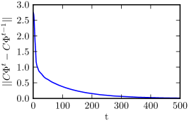
Figure 2: Stabilization of the probability distribution of the queue length After 500 step, the probability distribution of the queue is stable.

The state of the queue reaches lower and upper barriers. In each subsequent time step the likelihood of barriers increases and the remaining probabilities converge to zero. The probability distribution of the queue length depends on the initial state. The choice of half-filled state the queue determines the place of the middle peak of the likelihood, as shown in the Fig. 3.

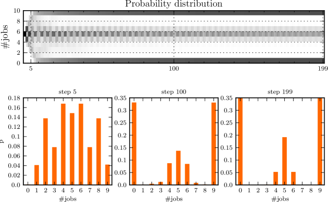
Figure 3: The probability distribution of the queue length with Hadamard coins. Up to $5$ step, evolution of the quantum queue behaves unitarily. Next, the probability of the queue lengths are distributed at the barriers. The middle peak is the result of choice of the initial state (18).

6 Classical system as special case of quantum systems.

In a particular case, formalism of discrete time quantum queues can be used to describe behaviour of a simple classical queueing system. Classical coin may be seen as a probability distribution over number of jobs flowing into the system and jobs processed. Quantum analogue of classical coin is a quantum channel that transforms any quantum state into diagonal state. The quantum description is of course in this case extremely inefficient due to large number of excessive parameters.

In order to reduce a quantum queuing system to classical one each step of the evolution a new coin uncorrelated with the state of the queue has to be introduced. It can be done by setting $\Phi_{C}$ to a composition of two channels: first one that traces out the coin systems $I$ and $O$, second one that introduces a coin transforming any quantum state into diagonal quantum state.

Transformation of quantum coin into a classic is performed by a quantum channel $\Phi_{D}$ in form

$$\Phi_{D}(\rho)=\sum_{x=0}^{D_{I}\times D_{O}-1}|x\rangle\langle x|\rho|x\rangle\langle x|.$$ (20)

Thus classical queue is implemented using a coin of the form $\Phi_{D}\cdot\Phi_{C}$. Consider superoperator corresponding with the channel $\Phi_{D}$ given by

$$\hat{\Phi}_{D}=\sum_{x=0}^{{D_{I}}^{2}\times{D_{O}}^{2}-1}|x\rangle\langle x|\otimes|x\rangle\langle x|.$$ (21)

Any superoperator $\hat{\Phi}$ corresponding with quantum channel from $M$-dimensional space to $L$-dimensional can be presented as

$$\hat{\Phi}=\sum_{i,j}^{M}\sum_{k,l}^{L}c_{i,j,k,l}|k\rangle\langle i|\otimes|l\rangle\langle j|,$$ (22)

where $c_{i,j,k,l}\in\mathbb{C}$ are constants. In our case $M=L=N$.

Composition of $\hat{\Phi}_{D}$ and any superoperator $\hat{\Phi}$ is in the form

$$\hat{\Phi}_{D}\cdot\hat{\Phi}=\sum_{x,i,j,k,l}^{N}c_{i,j,k,l}(|x\rangle\langle x|\otimes|x\rangle\langle x|)(|k\rangle\langle i|\otimes|l\rangle\langle j|)$$ (23)

which is equivalent to

$$\hat{\Phi}_{D}\cdot\hat{\Phi}=\sum_{x,i,j}^{N}c_{i,j,x,x}|x\rangle\langle i|\otimes|x\rangle\langle j|.$$ (24)

Jamiołkowski representation [2] of $\hat{\Phi}_{D}\cdot\hat{\Phi}$ is given by the form

$$J(\hat{\Phi}_{D}\cdot\hat{\Phi})=\sum_{x,i,j}^{N}c_{i,j,x,x}|x\rangle\langle x|\otimes|i\rangle\langle j|.$$ (25)

From the property TP of quantum channels shows that $\mathrm{tr}_{1}J(\hat{\Phi}_{D}\cdot\hat{\Phi})=\mathbb{1}$ thus

$$\mathrm{tr}_{1}J(\hat{\Phi}_{D}\cdot\hat{\Phi})=\sum_{i,j}^{N}\left(\sum_{x}^{N}c_{i,j,x,x}\right)|i\rangle\langle j|=\sum_{i,j}\delta_{i,j}|i\rangle\langle j|.$$ (26)

Submatrix determined by elements

$$[c_{i,i,x,x}]_{i,x=0}^{N-1}$$ (27)

is stochastic [4]. Thus coin of the form $\Phi_{D}\cdot\Phi_{C}$ simulates the classical queueing system.

Example 2

Let’s set the queue length dimension $D_{Q}=10$, it means that maximal length of queue can be $9$ and let’s fix dimensions of registers used to evaluating flow of jobs into the system in single time step $D_{I}=2$ and jobs processed in single time step $D_{O}=2$. Initially, the probability distribution of the queue length is unimodal and has “symmetric Bell” shape. Next, the distribution begins to unify and after $49$ steps, the probability distribution is close to the uniform distribution (Fig. 4).

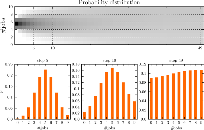
Figure 4: The probability distribution of the queue length with classical coin. At the beginning, the probability distribution of the queue length is unimodal. After $49$ steps the probability distribution is close to the uniform distribution.

In classical Queueing Theory length of the queues can have different probability distribution, e.g. Poisson distribution, Erlang distribution. Quantum queues can also have various probability distribution of length depending on the stochastic matrix (27).

7 The mean probability distribution of the queue length

Consider queuing system performed by mapping $\Phi$ such that $\lim_{t\to\infty}C\Phi^{t}$ is convergent, where $C$ is the partial trace and von Neumann measurement performed over subsystem $Q$. The probability distribution of the queue length is stationary and depend on the initial state $\rho$. Using the Monte Carlo method it is possible to calculate the mean probability distribution of the queue length for every initial state $\rho$. Consider the set of random states $\Omega$ and a Hilbert-Schmidt measure $\mu$ discussed in Subsection 4.2, then the mean probability distribution of the queue length over initial states from $\Omega$ is given by

$$\lim_{t\to\infty}\int_{\Omega}C\Phi^{t}(\rho)d\mu(\rho).$$ (28)

Example 3

Let the sizes of registers used to evaluating flow of jobs into system and jobs processed in single time step be $D_{I}=4$, $D_{O}=4$, respectively. Let’s fix the register dimension of queue length $D_{Q}$ to $10$ in single time step and $\Omega$ as a set of mixed random states. Quantum random walks are simulated using the Walsh-Hadamard, Grover and $DFT$ coins. More precisely, in each case QRW are simulated by coin operator given as

$$\Phi_{U}(\rho)=(U^{I}\otimes U^{O}\otimes\mathbb{1}^{Q})\rho(U^{I}\otimes U^{O}\otimes\mathbb{1}^{Q})^{\dagger},$$ (29)

where $U$ is a one of the above coin. For the $600~{}000$ initial mixed random states obtained the following mean probability distributions of the queue length.

Case 1

In the first case, quantum random walks been implemented via a Walsh-Hadamrd coin $H_{n}=\frac{1}{\sqrt{2}}\left(\begin{smallmatrix}1&1\\ 1&-1\\ \end{smallmatrix}\right)^{\otimes n}$. In this example $n$ is equal to $2$ and the mean probability distributions of the queue length is presented in Fig 5.

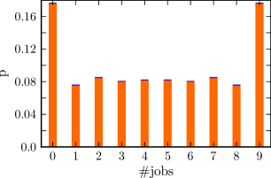
Figure 5: The mean probability distribution of the queue length with Walsh-Hadamard coin.

Case 2

In the second case, QRW are simulated using the Grover coin

$$G=\begin{pmatrix}\frac{2}{d}-1&\frac{2}{d}&\dots&\frac{2}{d}\\ \frac{2}{d}&\frac{2}{d}-1&\dots&\frac{2}{d}\\ \vdots&\vdots&\ddots&\vdots\\ \frac{2}{d}&\frac{2}{d}&\dots&\frac{2}{d}-1\end{pmatrix},$$ (30)

where in our case $d=4$ and results are shown in Fig. 6.

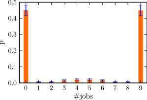
Figure 6: The mean probability distribution of the queue length with Grover coin. Error bars indicate plus minus one standard deviation.

Case 3

In the third case, quantum random walks are realized by DFT-coin

$$D=\frac{1}{\sqrt{d}}\begin{pmatrix}1&1&1&\dots&1\\ 1&\omega&\omega^{2}&\dots&\omega^{d-1}\\ \vdots&\vdots&\vdots&\ddots&\vdots\\ 1&\omega^{d-1}&\omega^{2(d-1)}&\dots&\omega^{(d-1)(d-1)}\end{pmatrix},$$ (31)

where $d=4$. For this coin, the mean probability distributions of the queue length is shown in Fig. 7.

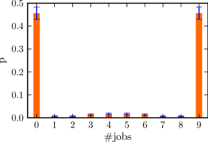
Figure 7: The mean probability distribution of the queue length with DFT coin. Error bars indicate plus minus one standard deviation.

The coins selection affects the probability distribution of the queue length. For this coins the standard deviations are relatively low so that the mean probability distribution of the queue length is a good estimator of queue length. While in case of Hadamard coin standard deviations are of the order of $10^{-12}$, thus initial states have little impact on queue length.

8 Conclusions

We have presented an extension of a simple queuing model based on Discrete Time Quantum Markov Chains using approch similar to Quantum Random Walks. We have shown that our model reduces to the classical one. We have proposed a methodology of analysis for quantum queuing models based on quantum channels and random mixed states.

In cases we studied numerically we observed that quantum queues models behave in a fundamentally different way than classical models of classical queues. In quantum models the length of the queue tends to quickly reach the barriers and stay in them, while classical balanced models tend to steady state in form of flat distribution.

The spectral structure of quantum models is much more complicated than that of classical ones. For most cases of queueing systems modelled using Discrete Time Markov Chain there exists steady state distribution. We have shown that for our models of quantum queues steady state distribution might exits but is dependent on the initial state of the modelled system. Therefore we proposed to analyse such systems using random initial mixed quantum state.

References

- [1] E Bach, S Copersmith, M. P. Goldschen, R. Joynt, and J. Watrous. One-dimensional quantum walks with absorbing boundaries. Journal of Computer and System Sciences, 69(4):562–592, 2004.
- [2] I. Bengtsson and K. Życzkowski. Geometry of Quantum States: An Introduction to Quantum Entanglement. Cambridge University Press, 1 edition, 2008.
- [3] D.S. Bernstein and S.P. Bhat. Lyapunov stability, semistability, and asymptotic stability of matrix second-order systems. In American Control Conference, 1994, volume 2, pages 2355–2359. IEEE, 1994.
- [4] W. Bruzda, V. Cappellini, H.J. Sommers, and K. Życzkowski. Random quantum operations. Physics Letters A, 373(3):320–324, 2009.
- [5] P. Gawron, J. Klamka, and R. Winiarczyk. Noise effects in the quantum search algorithm from the viewpoint of computational complexity. Int. J. Appl. Math. Comput. Sci, 22(2):493–499, 2012.
- [6] J. Kempe. Quantum random walks: an introductory overview. Contemporary Physics, 44(4):307–327, 2003.
- [7] Z. Puchała and J. A. Miszczak. Probability measure generated by the superfidelity. Journal of Physics A: Mathematical and Theoretical, 44:405301, 2011.
- [8] Z. Puchała, J.A. Miszczak, P. Gawron, and B. Gardas. Experimentally feasible measures of distance between quantum operations. Quantum Information Processing, 10(1):1–12, 2011.