Eliminating Electromagnetic Scattering from Small Particles

Abstract

This paper presents and discusses the conditions for zero electromagnetic scattering by electrically small particles. We consider the most general bi-anisotropic particles, characterized by four dyadic polarizabilities and study the case of uniaxially symmetric objects. Conditions for zero backward and forward scattering are found for a general uniaxial bi-anisotropic particle and specialized for all fundamental classes of bi-anisotropic particles: omega, “moving”, chiral, and Tellegen particles. Possibility for zero total scattering is also discussed for aforementioned cases. The scattering pattern and polarization of the scattered wave are also determined for each particle class. In particular, we analyze the interplay between different scattering mechanisms and show that in some cases it is possible to compensate scattering from a polarizable particle by appropriate magneto-electric coupling. Examples of particles providing zero backscattering and zero forward scattering are presented and studied numerically.

I Introduction

Examples of finite-sized objects with zero backscattering are known from the literature, a classical one being an object from an isotropic material with equal relative constitutive parameters, $\mu_{\text{r}}=\epsilon_{\text{r}}$, and $\pi/2$ rotational symmetry when observed from the incidence direction. [1, 2] The formal condition for zero forward scattering in the case of a small isotropic sphere was found in [3] and further discussed in [4, 5]. The last few years saw renewed interest in “invisible” objects in the context of the concept of cloaking (e.g., [6, 7, 8]), where the objects produce, in the ideal case, zero total scattered power. In papers on cloaking, the zero-scattering property is achieved either by using a material with such electromagnetic properties that the generated scattered wave interferes destructively with the wave scattered from the cloaked object (scattering-cancelation technique [6]) or by using inhomogeneous distributions of materials with exotic electromagnetic properties to create a volume inside which the incident wave cannot penetrate (transformation-optics technique [7, 8]). Alternatively, mesh-like objects can also be cloaked by guiding the wave through the object via a transmission-line network (transmission-line cloaking [9]).

Electromagnetic scattering from electrically small particles is determined by the lowest-order moments of induced current or polarization, the electric and magnetic dipole moments. If the particle material is an isotropic magnetodielectric, then the only possibility to achieve zero backscattering is basically the trivial case of equal relative parameters and proper symmetry of the particle shape [1, 2]. Similarly, the only possible solution for zero forward scattering by a small magnetodielectric sphere is the case found by Kerker [3]: $\epsilon_{\text{r}}=(4-\mu_{\text{r}})/(2\mu_{\text{r}}+1)$, which in actuality corresponds only to greatly diminished, but not identically zero, forward scattering [5, 10]. Recently, it was shown theoretically [10, 11, 12] and confirmed by microwave experiments [13, 14] that electric and magnetic polarizabilities required for forming a zero-scattering Huygens pair of dipoles satisfying Kerker’s conditions can be realized in a single dielectric sphere. In antenna engineering, several realizations of small antennas satisfying the zero-backscattering condition, analogous to the Kerker condition for an isotropic sphere, are known [15, 16, 17, 18].

However, electrically small particles can exhibit bi-anisotropic magneto-electric coupling (e.g.,  [19]), so that the electric moment of the particle is generated by both electric and magnetic incident fields (likewise, the magnetic moment is induced by both fields). We expect that bi-anisotropy of particles can offer more possibilities for controlling scattering, in particular, for realizing non-scattering objects.

In this paper, we study zero-scattering conditions (in back and forward directions) for general bi-anisotropic particles, including both reciprocal and nonreciprocal polarizabilities and field-coupling mechanisms. We assume that the particles are electrically small, so that the dipole approximation is an appropriate model of the particle response and write the relations between the induced electric and magnetic dipole moments $\mathbf{p}$ and $\mathbf{m}$ in terms of four dyadic polarizabilities $\overline{\overline{\alpha}}$:

$$\mathbf{p} = \overline{\overline{\alpha}}_{\text{ee}}\cdot\mathbf{E}_{\text{inc}}+\overline{\overline{\alpha}}_{\text{em}}\cdot\mathbf{H}_{\text{inc}},$$ (1)

$$\mathbf{m} = \overline{\overline{\alpha}}_{\text{me}}\cdot\mathbf{E}_{\text{inc}}+\overline{\overline{\alpha}}_{\text{mm}}\cdot\mathbf{H}_{\text{inc}}.$$ (2)

Here, $\mathbf{E}_{\text{inc}}$ and $\mathbf{H}_{\text{inc}}$ are the incident fields. In earlier studies, conditions for zero backscattering from isotropic chiral objects were found [20, 21, 22], and a uniaxial chiral object with low backscattering was investigated [23]. In a recent paper [24] zero-backscattering from bi-anisotropic objects was mentioned in the context of scattering from objects made from self-dual materials. It has been shown that in addition to the $\pi/2$ rotational symmetry, self-dual nature of the bi-anisotropic filling material is sufficient for zero backscattering. In terms of the particle polarizabilities, self-duality conditions lead to the requirements $\overline{\overline{\alpha}}_{\text{mm}}=\eta_{0}^{2}\overline{\overline{\alpha}}_{\text{ee}}$ and $\overline{\overline{\alpha}}_{\text{em}}=-\overline{\overline{\alpha}}_{\text{me}}$, where $\eta_{0}$ is the free-space wave impedance [22]. As examples of self-dual objects, a so called DB sphere was studied in [25], and a D’B’ sphere and cube in [24]. Furthermore, it was shown in [24] that the physical geometry of the object does not need to have the $\pi/2$ rotational symmetry, as long as the geometrical asymmetry is balanced by anisotropy of material response.

In the following, the scattering properties of a general uniaxial bi-anisotropic particle are analyzed and the required conditions for achieving zero backscattering, zero forward scattering as well as zero total scattering (i.e., invisibility) are derived. The fundamental classes of uniaxial bi-anisotropic particles (omega, “moving”, chiral, and Tellegen particles) are studied systematically, and the aforementioned zero scattering conditions for each particle class are derived. Furthermore, two concrete particle designs, one corresponding to zero backscattering and the other one to zero forward scattering, are presented and studied numerically. In our analysis, the incident wave is assumed to be linearly polarized. This study is relevant to the design of absorbers, where the goal is to minimize reflection and/or transmission and to the design of cloaks and low-scattering small sensors, where the goal is to minimize the total scattering.

II Scattering from Electrically Small Bi-Anisotropic Particles

II-A Polarizabilities and the Scattering Amplitude

Scattered fields from a single electrically small bi-anisotropic scatterer illuminated by an incident plane wave can be analyzed based on the induced electric and magnetic dipole moments whose relations to the incident electromagnetic fields are defined by (1) and (2). For a reciprocal particle, we have [19]:

$$\overline{\overline{\alpha}}_{\text{ee}}=\overline{\overline{\alpha}}_{\text{ee}}^{T},\quad\overline{\overline{\alpha}}_{\text{mm}}=\overline{\overline{\alpha}}_{\text{mm}}^{T},\quad\text{and}\quad\overline{\overline{\alpha}}_{\text{em}}=-\overline{\overline{\alpha}}_{\text{me}}^{T}$$ (3)

and for a lossless particle

$$\overline{\overline{\alpha}}_{\text{ee}}=\overline{\overline{\alpha}}_{\text{ee}}^{\dagger},\quad\overline{\overline{\alpha}}_{\text{mm}}=\overline{\overline{\alpha}}_{\text{mm}}^{\dagger},\quad\text{and}\quad\overline{\overline{\alpha}}_{\text{em}}=\overline{\overline{\alpha}}_{\text{me}}^{\dagger},$$ (4)

where $T$ denotes the transpose operation and ${\dagger}$ is the Hermitian operator (transpose of the complex conjugate). However, as we want to study the scattering from a particle, we should deal with the dynamic polarizabilities (the quasi-static model will be not adequate) and include scattering loss in the consideration, even for a “lossless” particle (particle with no absorption losses). In the last case, the polarizability dyadics are governed by the following set of equations following from the law of energy conservation [26]:

$$\textnormal{Im}\{(\overline{\overline{\alpha}}_{\text{ee}}-\overline{\overline{\alpha}}_{\text{em}}\cdot\overline{\overline{\alpha}}_{\text{mm}}^{-1}\cdot\overline{\overline{\alpha}}_{\text{me}})^{-1}\}=\frac{k}{6\pi\epsilon_{0}}\overline{\overline{I}},$$ (5)

$$\textnormal{Im}\{(\overline{\overline{\alpha}}_{\text{mm}}-\overline{\overline{\alpha}}_{\text{me}}\cdot\overline{\overline{\alpha}}_{\text{ee}}^{-1}\cdot\overline{\overline{\alpha}}_{\text{em}})^{-1}\}=\frac{k}{6\pi\mu_{0}}\overline{\overline{I}},$$ (6)

$$\textnormal{Re}\{(\overline{\overline{\alpha}}_{\text{ee}}-\overline{\overline{\alpha}}_{\text{em}}\cdot\overline{\overline{\alpha}}_{\text{mm}}^{-1}\cdot\overline{\overline{\alpha}}_{\text{me}})^{-1}\cdot\overline{\overline{\alpha}}_{\text{em}}\cdot\overline{\overline{\alpha}}_{\text{mm}}^{-1}\}=0,$$ (7)

$$\textnormal{Re}\{(\overline{\overline{\alpha}}_{\text{mm}}-\overline{\overline{\alpha}}_{\text{me}}\cdot\overline{\overline{\alpha}}_{\text{ee}}^{-1}\cdot\overline{\overline{\alpha}}_{\text{em}})^{-1}\cdot\overline{\overline{\alpha}}_{\text{me}}\cdot\overline{\overline{\alpha}}_{\text{ee}}^{-1}\}=0.$$ (8)

Here, $k$ is the free-space wavenumber and $\overline{\overline{I}}$ is the three-dimensional unit dyadic. In the limiting case of ideal planar particles when the fields along the axial direction do not interact with the particle, $2\times 2$ dyadics can and should be used in (5)–(8) in order to avoid singular dyadics. For a reciprocal particle, the last two equations are equivalent, and this is true also for all non-absorbing nonreciprocal uniaxial particles analyzed in this paper. It should be noted that due to the inclusion of scattering losses all the polarizabilities can be complex quantities whereas if the scattering losses are excluded for lossless particles, $\overline{\overline{\alpha}}_{\text{ee}}$ and $\overline{\overline{\alpha}}_{\text{mm}}$ are always purely real while $\overline{\overline{\alpha}}_{\text{em}}$ and $\overline{\overline{\alpha}}_{\text{me}}$ are purely imaginary for a reciprocal particle and purely real for a nonreciprocal particle with $\overline{\overline{\alpha}}_{\text{em}}=-\overline{\overline{\alpha}}_{\text{me}}^{\dagger}$.

The scattered electric far field from electric and magnetic dipole moments ($\mathbf{p}$ and $\mathbf{m}$) at the origin can be written as [24, 27]

$$\mathbf{E}_{\text{sca}}=-\omega^{2}\mu_{0}\frac{e^{-jkr}}{4\pi r}\mathbf{F}_{\text{sca}},$$ (9)

where the radiation vector $\mathbf{F}_{\text{sca}}$ reads

$$\mathbf{F}_{\text{sca}}=\mathbf{u}_{r}\times(\mathbf{u}_{r}\times\mathbf{p})+\mathbf{u}_{r}\times\frac{\mathbf{m}}{\eta_{0}},$$ (10)

$\mathbf{u}_{r}$ is unit vector in the scattering direction, $\eta_{0}$ is the wave impedance of free space, and $r$ is the radial distance from the origin. The normalized scattering pattern $\mathbf{F}_{\text{sca, norm}}$ for a given particle is given simply by $\mathbf{F}_{\text{sca}}/\max\{|\mathbf{F}_{\text{sca}}|\}$ as a function of the observation angles. Scattering directivity pattern, on the other hand, is defined as ratio of the power density the scatterer radiates in a given direction and the power density radiated by an ideal isotropic radiator radiating the same total power and is given by

$$D=\frac{|\mathbf{F}_{\text{sca,norm}}|^{2}}{\frac{1}{4\pi}\int^{2\pi}_{0}\int^{\pi}_{0}|\mathbf{F}_{\text{sca, norm}}|^{2}d\theta d\phi},$$ (11)

where $\theta$ and $\phi$ are the inclination and azimuthal angles of a spherical coordinate system, respectively.

II-B Zero Scattering under Plane-Wave Illumination: General Conditions

Zero scattering in a certain direction for a given configuration of exciting fields can be studied by demanding $\mathbf{F}_{\text{sca}}=0$ in (10) and using the relation between the fields of the incident plane wave

$$\mathbf{H}_{\text{inc}}=\frac{\mathbf{k}}{\omega\mu_{0}}\times\mathbf{E}_{\text{inc}}=\frac{1}{\eta_{0}}\mathbf{u}\times\mathbf{E}_{\text{inc}},$$ (12)

where $\mathbf{u}$ is the incidence direction. This leads to the condition

$$\mathbf{u}_{r}\times\overline{\overline{\alpha}}_{\text{ee}}\cdot\mathbf{E}_{\text{inc}}+\mathbf{u}_{r}\times\frac{1}{\eta_{0}}\overline{\overline{\alpha}}_{\text{em}}\cdot(\mathbf{u}\times\mathbf{E}_{\text{inc}})$$ (13)

$$\ \ \ \ +\frac{1}{\eta_{0}}\overline{\overline{\alpha}}_{\text{me}}\cdot\mathbf{E}_{\text{inc}}+\frac{1}{\eta_{0}^{2}}\overline{\overline{\alpha}}_{\text{mm}}\cdot(\mathbf{u}\times\mathbf{E}_{\text{inc}})=0.\hskip 14.22636pt$$

We can rewrite the term $\overline{\overline{\alpha}}\cdot(\mathbf{u}\times\mathbf{E}_{\text{inc}})$ as $(\overline{\overline{\alpha}}\times\mathbf{u})\cdot\mathbf{E}_{\text{inc}}$, which allows us to write the condition in a convenient form:

$$(\mathbf{u}_{r}\times\overline{\overline{\alpha}}_{\text{ee}}+\hbox to0.0pt{$\displaystyle\mathbf{u}_{r}\times\frac{1}{\eta_{0}}\left(\overline{\overline{\alpha}}_{\text{em}}\times\mathbf{u}\right)+\frac{1}{\eta_{0}}\overline{\overline{\alpha}}_{\text{me}}$\hss}$$ (14)

$$\ \ \ \ +\frac{1}{\eta_{0}^{2}}\left(\overline{\overline{\alpha}}_{\text{mm}}\times\mathbf{u}\right))\cdot\mathbf{E}_{\text{inc}}=0.\hskip 14.22636pt$$

For the condition of zero backscattering we demand $\mathbf{u}_{r}=-\mathbf{u}$ and get

$$-\mathbf{u}\times\overline{\overline{\alpha}}_{\text{ee}}-\mathbf{u}\times\frac{1}{\eta_{0}}\overline{\overline{\alpha}}_{\text{em}}\times\mathbf{u}+\frac{1}{\eta_{0}}\overline{\overline{\alpha}}_{\text{me}}+\frac{1}{\eta_{0}^{2}}\overline{\overline{\alpha}}_{\text{mm}}\times\mathbf{u}=0.$$ (15)

To find the condition for zero forward scattering we demand in turn $\mathbf{u}_{r}=\mathbf{u}$ and get

$$\mathbf{u}\times\overline{\overline{\alpha}}_{\text{ee}}+\mathbf{u}\times\frac{1}{\eta_{0}}\overline{\overline{\alpha}}_{\text{em}}\times\mathbf{u}+\frac{1}{\eta_{0}}\overline{\overline{\alpha}}_{\text{me}}+\frac{1}{\eta_{0}^{2}}\overline{\overline{\alpha}}_{\text{mm}}\times\mathbf{u}=0.$$ (16)

III Particles under Study

In this paper we study the zero-scattering conditions (15) and (16) when the scatterer is a uniaxial bi-anisotropic particle. The case of uniaxial (rotational) symmetry is chosen in view of having zero scattering for any polarization direction of the incident field. In view of potential applications in periodical arrays at normal incidence we concentrate on the effects of polarizabilities in the transverse plane and do not include the axial polarizabilities in the analysis. In the most general bi-anisotropic case, the transverse polarizabilities in (1) and (2) take the forms

$$\overline{\overline{\alpha}}_{\text{ee}} = \alpha_{\text{ee,S}}\overline{\overline{I}}_{\text{t}}+\alpha_{\text{ee,A}}\overline{\overline{J}}_{\text{t}},$$ (17)

$$\overline{\overline{\alpha}}_{\text{mm}} = \alpha_{\text{mm,S}}\overline{\overline{I}}_{\text{t}}+\alpha_{\text{mm,A}}\overline{\overline{J}}_{\text{t}}.$$ (18)

$$\overline{\overline{\alpha}}_{\text{em}} = \alpha_{\text{em,S}}\overline{\overline{I}}_{\text{t}}+\alpha_{\text{em,A}}\overline{\overline{J}}_{\text{t}},$$ (19)

$$\overline{\overline{\alpha}}_{\text{me}} = \alpha_{\text{me,S}}\overline{\overline{I}}_{\text{t}}+\alpha_{\text{me,A}}\overline{\overline{J}}_{\text{t}},$$ (20)

where S and A refer, respectively, to the symmetric and antisymmetric parts of the corresponding dyadics, $\overline{\overline{I}}_{\text{t}}$ is the transverse unit dyadic, that is, a dyadic of the form ${\overline{\overline{I}}_{\text{t}}=\overline{\overline{I}}-\mathbf{u}_{z}\mathbf{u}_{z}}$, ${\overline{\overline{J}}_{\text{t}}=\mathbf{u}_{z}\times\overline{\overline{I}}_{\text{t}}}$ is the vector-product operator, and $\mathbf{u}_{z}$ is the unit vector along the particle axis. In addition to the general case, we will consider in detail the four canonical bi-anisotropic particles as classified in [19, 28]: omega, “moving”, chiral, and Tellegen particles. Omega and chiral particles are, based on (3), reciprocal particles, whereas “moving” and Tellegen particles are nonreciprocal. These four types are distinguished from each other solely by the values of the symmetric and antisymmetric cross-coupling polarizability components as shown in Table I.

TABLE I: Different types of uniaxial bi-anisotropic particles ($\alpha$ can be any complex number).

	$\alpha_{\text{em,S}}$	$\alpha_{\text{em,A}}$	$\alpha_{\text{me,S}}$	$\alpha_{\text{me,A}}$
Omega particle	$0$	$\alpha$	$0$	$\alpha$
“Moving” particle	$0$	$\alpha$	$0$	$-\alpha$
Chiral particle	$\alpha$	$0$	$-\alpha$	$0$
Tellegen particle	$\alpha$	$0$	$\alpha$	$0$

III-A General Uniaxial Particle

First, let us consider the most general uniaxial bi-anisotropic particle by allowing all the polarizabilities, $\overline{\overline{\alpha}}_{\text{ee}}$, $\overline{\overline{\alpha}}_{\text{mm}}$, $\overline{\overline{\alpha}}_{\text{em}}$ and $\overline{\overline{\alpha}}_{\text{me}}$, to have both symmetric and antisymmetric parts as defined in (17)–(20).

III-A1 Zero Backscattering

In this general case, the zero backscattering condition (15) reduces to

$$-\alpha_{\text{ee,S}}(\mathbf{u}\times\overline{\overline{I}}_{\text{t}})-\alpha_{\text{ee,A}}(\mathbf{u}\times\overline{\overline{J}}_{\text{t}})$$ (21)

$$\ \ \ -\frac{\alpha_{\text{em,S}}}{\eta_{0}}(\mathbf{u}\times\overline{\overline{I}}_{\text{t}}\times\mathbf{u})-\frac{\alpha_{\text{em,A}}}{\eta_{0}}(\mathbf{u}\times\overline{\overline{J}}_{\text{t}}\times\mathbf{u})$$

$$\ \ \ +\frac{\alpha_{\text{me,S}}}{\eta_{0}}\overline{\overline{I}}_{\text{t}}+\frac{\alpha_{\text{me,A}}}{\eta_{0}}\overline{\overline{J}}_{\text{t}}$$

$$\ \ \ +\frac{\alpha_{\text{mm,S}}}{\eta_{0}^{2}}(\overline{\overline{I}}_{\text{t}}\times\mathbf{u})+\frac{\alpha_{\text{mm,A}}}{\eta_{0}^{2}}(\overline{\overline{J}}_{\text{t}}\times\mathbf{u})=0.$$

By plugging a general directional vector $\mathbf{u}=\sin{\theta}\cos{\phi}\mathbf{u}_{x}+\sin{\theta}\sin{\phi}\mathbf{u}_{y}+\cos{\theta}\mathbf{u}_{z}=A\mathbf{u}_{x}+B\mathbf{u}_{y}+C\mathbf{u}_{z}$ into (21), we can write a separate scalar equation for each of the nine dyadic components. It turns out that (21) for non-axial incidence can be satisfied only for certain special cases, namely when we have

$$\alpha_{\text{em,S}}=\alpha_{\text{me,S}}=\alpha_{\text{ee,A}}=\alpha_{\text{mm,A}}=0,$$ (22)

$$\alpha_{\text{ee,S}}=\frac{\alpha_{\text{em,A}}}{\eta}C=\frac{\alpha_{\text{me,A}}}{\eta}\frac{1}{C}=-\frac{\alpha_{\text{mm,S}}}{\eta^{2}}.$$ (23)

Notably even in this case, zero backscattering can be achieved for only one angle of incidence with given polarizabilities, and for the incident direction orthogonal to the axis of the particle this is not possible at all. Also, it was assumed that particle is ideally uniaxial meaning that the polarizability dyadics have no component along the particle axis ($\mathbf{u}_{\text{z}}\mathbf{u}_{\text{z}}$-component). If this component would be included, no solution could be found for oblique incidence.

For the axial incidence ($A=B=0$, $C=\pm 1$) using the identities $\mathbf{u}_{\text{z}}\times\overline{\overline{I}}_{\text{t}}=\overline{\overline{I}}_{\text{t}}\times\mathbf{u}_{\text{z}}=\overline{\overline{J}}_{\text{t}}$, $\mathbf{u}_{\text{z}}\times\overline{\overline{I}}_{\text{t}}\times\mathbf{u}_{\text{z}}=-\overline{\overline{I}}_{\text{t}}$, and $\mathbf{u}_{\text{z}}\times\overline{\overline{J}}_{\text{t}}\times\mathbf{u}_{\text{z}}=-\overline{\overline{J}}_{\text{t}}$, the dyadic equation (21) reduces to two scalar equations:

$$\mp\alpha_{\text{ee,S}}\pm\frac{\alpha_{\text{mm,S}}}{\eta_{0}^{2}}+\frac{\alpha_{\text{em,A}}}{\eta_{0}}+\frac{\alpha_{\text{me,A}}}{\eta_{0}} = 0,$$ (24)

$$\pm\alpha_{\text{ee,A}}\mp\frac{\alpha_{\text{mm,A}}}{\eta_{0}^{2}}+\frac{\alpha_{\text{em,S}}}{\eta_{0}}+\frac{\alpha_{\text{me,S}}}{\eta_{0}} = 0.$$ (25)

Here, the top sign corresponds to the incident-wave propagation along $+z$-direction and the bottom sign along $-z$-direction. It can be seen that the symmetric parts of the cross-coupling polarizabilities are connected to the antisymmetric parts of the electric and magnetic polarizabilities and vice versa. This is easily understood by looking at the basic equations for the dipole moments (1) and (2) as the electric and magnetic fields are orthogonal to each other in a plane wave and the antisymmetric dyadic $\overline{\overline{J}}_{\text{t}}$ corresponds to a 90^∘ counterclockwise rotation around the $z$-axis.

In the simplest special case of isotropic reciprocal particles the above relations reduce to $\mp\alpha_{\text{ee,S}}\pm\frac{\alpha_{\text{mm,S}}}{\eta_{0}^{2}}=0$, which simply means that the electric and magnetic polarizabilities should be balanced in order to ensure the Huygens’ relation between the induced moments. For bi-anisotropic reciprocal particles, we see from the first relation that an imbalance between these two polarizabilities can be compensated by properly choosing the omega coupling coefficient $\alpha_{\text{em,A}}$ (or $\alpha_{\text{me,A}}$ as we have $\alpha_{\text{em,A}}=\alpha_{\text{me,A}}$ for omega particles). Basically, this tells us that the required balance between the induced electric and magnetic moments can be be achieved using the omega coupling effect instead or in addition to the magnetization induced by incident magnetic fields. This may be important and beneficial for applications, because the omega coupling effect is a first-order spatial dispersion effect, which is usually much stronger than the second-order magnetization effect. The second relation tells us that for reciprocal particles the zero backscattering property is independent of the chirality parameter $\alpha_{\text{em,S}}$ as we have $\alpha_{\text{ee,A}}=\alpha_{\text{mm,A}}=0$ and $\alpha_{\text{em,S}}=-\alpha_{\text{me,S}}$ by definition.

Nonreciprocal particles can have non-zero antisymmetric parts of electric and magnetic polarizabilities (e.g., magnetized ferrite spheres). For particles without bi-anisotropic coupling, the second relation tells that if the antisymmetric parts do not satisfy $\pm\alpha_{\text{ee,A}}\mp\frac{\alpha_{\text{mm,A}}}{\eta_{0}^{2}}=0$, zero backscattering cannot be achieved. In particular, this is the case when only one of the polarizabilities exhibits nonreciprocity, but the other one is purely symmetric (as in the same example of a ferrite sphere). An important conclusion from this relation is that backscattering due to nonreciprocity in electric and/or magnetic response can be compensated by introducing magneto-electric coupling of the Tellegen type ($\alpha_{\text{em,S}}=\alpha_{\text{me,S}}$).

III-A2 Zero Forward Scattering

Similarly, the conditions for zero forward scattering can be derived based on (16). The condition for zero forward scattering with arbitrary incidence direction reads

$$\alpha_{\text{ee,S}}(\mathbf{u}\times\overline{\overline{I}}_{\text{t}})+\alpha_{\text{ee,A}}(\mathbf{u}\times\overline{\overline{J}}_{\text{t}})$$ (26)

$$\ \ \ +\frac{\alpha_{\text{em,S}}}{\eta_{0}}(\mathbf{u}\times\overline{\overline{I}}_{\text{t}}\times\mathbf{u})+\frac{\alpha_{\text{em,A}}}{\eta_{0}}(\mathbf{u}\times\overline{\overline{J}}_{\text{t}}\times\mathbf{u})$$

$$\ \ \ +\frac{\alpha_{\text{me,S}}}{\eta_{0}}\overline{\overline{I}}_{\text{t}}+\frac{\alpha_{\text{me,A}}}{\eta_{0}}\overline{\overline{J}}_{\text{t}}$$

$$\ \ \ +\frac{\alpha_{\text{mm,S}}}{\eta_{0}^{2}}(\overline{\overline{I}}_{\text{t}}\times\mathbf{u})+\frac{\alpha_{\text{mm,A}}}{\eta_{0}^{2}}(\overline{\overline{J}}_{\text{t}}\times\mathbf{u})=0.$$

Again, by plugging a general directional vector $\mathbf{u}=\sin{\theta}\cos{\phi}\mathbf{u}_{x}+\sin{\theta}\sin{\phi}\mathbf{u}_{y}+\cos{\theta}\mathbf{u}_{z}=A\mathbf{u}_{x}+B\mathbf{u}_{y}+C\mathbf{u}_{z}$ into (26), conditions can be derived for zero forward scattering with non-axial incidence:

$$\alpha_{\text{em,S}}=\alpha_{\text{me,S}}=\alpha_{\text{ee,A}}=\alpha_{\text{mm,A}}=0,$$ (27)

$$\alpha_{\text{ee,S}}=\frac{\alpha_{\text{em,A}}}{\eta}C=-\frac{\alpha_{\text{me,A}}}{\eta}\frac{1}{C}=\frac{\alpha_{\text{mm,S}}}{\eta^{2}}.\hskip 22.76228pt$$ (28)

As with zero backscattering, only one angle of incidence can be covered with given polarizabilities and this solution is only valid for an ideally uniaxial particle.

For the axial incidence, we get two scalar equations:

$$\pm\alpha_{\text{ee,S}}\pm\frac{\alpha_{\text{mm,S}}}{\eta_{0}^{2}}-\frac{\alpha_{\text{em,A}}}{\eta_{0}}+\frac{\alpha_{\text{me,A}}}{\eta_{0}} = 0,\hskip 14.22636pt$$ (29)

$$\mp\alpha_{\text{ee,A}}\mp\frac{\alpha_{\text{mm,A}}}{\eta_{0}^{2}}-\frac{\alpha_{\text{em,S}}}{\eta_{0}}+\frac{\alpha_{\text{me,S}}}{\eta_{0}} = 0,$$ (30)

where, again, the top sign corresponds to the incident-wave propagation along $+z$-direction and the bottom sign along $-z$-direction. Notably, these conditions greatly resemble the conditions for zero backscattering with the only difference being the signs of some of the components.

In this case, an imbalance between the electric and magnetic polarizabilities (the first relation) can be compensated by magneto-electric coupling coefficient of a moving-particle type ($\alpha_{\text{em,A}}=-\alpha_{\text{me,A}}$). Forward scattering due to antisymmetric (nonreciprocal) parts of electric and magnetic polarizabilities can be compensated by making the particle chiral (i.e., introducing magneto-electric coupling of the type $\alpha_{\text{em,S}}=-\alpha_{\text{me,S}}$) and properly choosing the value of the chirality parameter (the second relation). In other words, nonreciprocal Faraday rotation in transmission can be compensated by reciprocal rotation due to the chirality of the particle.

III-A3 Zero Total Scattering

But what if we demand that both forward and backward scattering amplitudes are zero? By demanding all the equations (24), (25), (29), and (30) to be true, we get a set of four equations for the eight unknown polarizability components:

$$\alpha_{\text{ee,S}} = \pm\frac{\alpha_{\text{em,A}}}{\eta_{0}},$$ (31)

$$\alpha_{\text{mm,S}} = \mp\eta_{0}\alpha_{\text{me,A}},$$ (32)

$$\alpha_{\text{ee,A}} = \mp\frac{\alpha_{\text{em,S}}}{\eta_{0}},$$ (33)

$$\alpha_{\text{mm,A}} = \pm\eta_{0}\alpha_{\text{me,S}},$$ (34)

where the top sign corresponds to the incident-wave propagation along $+z$-direction and the bottom sign along $-z$-direction. By plugging (31)–(34) into (14), it can be seen that these conditions hold not only for zero scattering in the forward and backward directions but actually for zero scattering in all directions. Actually, if (31)–(34) are satisfied, the induced dipole moments are equal to zero. This means that such particles are not excited by plane waves propagating axially with the particle axis in one direction (i.e., no electric nor magnetic dipole moments induced), but they show non-zero total scattering when the incident wave is propagating in the opposite direction. In fact, it can be seen that for the opposite axial propagation direction the zero backscattering condition is satisfied as long as we have $\overline{\overline{\alpha}}_{\text{em}}=\overline{\overline{\alpha}}_{\text{me}}$. On the other hand, if we have $\overline{\overline{\alpha}}_{\text{em}}=-\overline{\overline{\alpha}}_{\text{me}}$, the zero forward scattering condition is satisfied instead.

As zero forward scattering property is governed by the optical theorem, the topic merits further investigation. Here, we will study passivity of zero forward scattering particles and clarify the physical meaning of the derived zero forward scattering conditions. The passivity of a particle can be studied by looking at the power spent by the incident wave for exciting the particle, which is given by [26]

$$P=\frac{1}{2}{\rm Re\mit}[{(j\omega\mathbf{p})^{*}\cdot\mathbf{E}_{\text{inc}}+j\omega\mathbf{m}\cdot\mathbf{H}_{\text{inc}}^{*}}].$$ (35)

If the particle absorbs power (some of which may be re-radiated by the particle), we have $P>0$ and if it generates power (i.e., is active), we have $P<0$. If we have $P=0$, there is no power exchange between the incident wave and the particle. By plugging the dipole moments generated by a general bi-anisotropic particle when the zero forward scattering conditions (29) and (30) are satisfied into (35), passivity of the particle can be analyzed.

Firstly, by using the definitions (17)–(20), equation (35) can be written as

$$P=\frac{1}{2}\omega|E_{\text{inc}}|^{2}{\rm Im\mit}\left[\alpha^{*}_{\text{ee,S}}\mp\frac{\alpha_{\text{em,A}}^{*}}{\eta_{0}}-\frac{\alpha_{\text{mm,S}}}{\eta_{0}^{2}}\mp\frac{\alpha_{\text{me,A}}}{\eta_{0}}\right],$$ (36)

where the top sign corresponds to propagation along $+z$-direction and the bottom sign along $-z$-direction. If we now enforce the zero forward scattering conditions (29) and (30), we see that the power absorbed by the particle is identically zero for any values of the polarizabilities. Note that the induced dipole moments are not zero, except if also the backward scattering is zero. Therefore, there is seemingly no power interaction between the incident wave and the particle. As the particle takes no power from the incident field, it cannot re-radiate any power either. Still, the particle is not necessarily invisible. This can be seen by looking at the power radiated by the particle [26]

$$P=\frac{\omega^{4}}{12\pi c}(\mu_{0}\mathbf{p}^{*}\cdot\mathbf{p}+\epsilon_{0}\mathbf{m}^{*}\cdot\mathbf{m}).$$ (37)

For a passive particle, this power should be equal to the power spent by the incident power for exciting the particle. However, the radiated power is zero only if the induced dipole moments are both zero and this is only true if the zero total scattering conditions are satisfied. Therefore, in order to have exactly zero forward scattering with non-zero total scattering, the particle has to be active. As discussed in [5, 10, 11], this does not exclude possibilities for achieving greatly reduced (but still not exactly zero) forward scattering with non-zero backward and total scattering. Basically, this is achieved when the real part of (29) is zero and the imaginary part of (30) is zero. Since the optical theorem is only valid for passive particles, the results presented in this paper are not in conflict with the optical theorem.

In the following, we specify the general results for all fundamental classes of bi-anisotropic particles.

III-B Uniaxial Omega Particle and Uniaxial Moving Particle

For a uniaxial omega particle along the $z$-axis, the polarizabilities have the form

$$\left\{\begin{array}[]{l}\displaystyle\overline{\overline{\alpha}}_{\text{ee}}=\alpha_{\text{ee}}\overline{\overline{I}}_{\text{t}}\vspace*{.2cm}\\ \displaystyle\overline{\overline{\alpha}}_{\text{mm}}=\alpha_{\text{mm}}\overline{\overline{I}}_{\text{t}}\vspace*{.2cm}\\ \displaystyle\overline{\overline{\alpha}}_{\text{em}}=\alpha_{\text{em}}\overline{\overline{J}}_{\text{t}}\vspace*{.2cm}\\ \displaystyle\overline{\overline{\alpha}}_{\text{me}}=\alpha_{\text{me}}\overline{\overline{J}}_{\text{t}},\end{array}\right.$$ (38)

that is, only the symmetric parts of $\overline{\overline{\alpha}}_{\text{ee}}$ and $\overline{\overline{\alpha}}_{\text{mm}}$ and antisymmetric parts of $\overline{\overline{\alpha}}_{\text{em}}$ and $\overline{\overline{\alpha}}_{\text{me}}$ are non-zero. The omega particle is reciprocal, i.e., we have

$$\overline{\overline{\alpha}}_{\text{em}}=\overline{\overline{\alpha}}_{\text{me}}=\alpha\overline{\overline{J}}_{\text{t}}.$$ (39)

Equations (38) hold also for a uniaxial “moving” particle (with the axis oriented along the $z$-axis), and it is, therefore, convenient to study these two classes together. However, as a uniaxial “moving” particle is nonreciprocal, we must enforce, instead of (39), the condition

$$\overline{\overline{\alpha}}_{\text{em}}=-\overline{\overline{\alpha}}_{\text{me}}=\alpha\overline{\overline{J}}_{\text{t}}.$$ (40)

“Moving” is set here inside quotation marks as the “moving” particle is not a particle in motion, but a nonreciprocal particle at rest with the polarizabilities in this form. These quotation marks are dropped in the rest of the paper for simplicity of notations.

III-B1 Zero Backscattering

Let us first consider backscattering from a single uniaxial omega or moving particle. As (22) and (23) are not satisfied, zero backscattering is not possible for oblique incidence for either particle. For the axial incidence ($\mathbf{u}=\pm\mathbf{u}_{z}$), the zero backscattering condition (24) simplifies to

$$-\alpha_{\text{ee}}\pm\frac{2}{\eta_{0}}\alpha+\frac{1}{\eta_{0}^{2}}\alpha_{\text{mm}}=0$$ (41)

for an omega particle and to

$$\alpha_{\text{ee}}=\frac{1}{\eta_{0}^{2}}\alpha_{\text{mm}},\quad\mbox{and arbitrary}\,\,\alpha$$ (42)

for a moving particle. Here, the $\pm$ signs correspond to the opposite directions of the incident plane wave ($\mathbf{u}=\pm\mathbf{u}_{z}$). The other zero backscattering condition (25) vanishes for both particles. As the scattering losses must be included according to (5)–(8), all the polarizabilities can be complex quantities even for a particle without absorption losses. Therefore, both equations can, at least in principle, be satisfied even if the absorption losses are excluded. However, if scattering and absorption losses are both excluded, (41) cannot be satisfied for $\alpha\neq 0$. It should be noted that the condition for moving particles holds also if the propagation direction is reversed despite of the inherent nonreciprocity of the particle. Also, as the self-duality conditions $\overline{\overline{\alpha}}_{\text{mm}}=\eta_{0}^{2}\overline{\overline{\alpha}}_{\text{ee}}$ and $\overline{\overline{\alpha}}_{\text{em}}=-\overline{\overline{\alpha}}_{\text{me}}$ as well as the $\pi/2$ rotational symmetry condition with the axial incidence are both satisfied by definition for a moving particle, we can conclude that the general conditions for zero backscattering derived in [24] hold for the moving particle case. On the other hand, by definition these conditions are not satisfied for an omega particle, as we have $\overline{\overline{\alpha}}_{\text{em}}=\overline{\overline{\alpha}}_{\text{me}}$, not $\overline{\overline{\alpha}}_{\text{em}}=-\overline{\overline{\alpha}}_{\text{me}}$. However, in [24] in deriving the self-duality condition the particles were assumed to be lossless. If the losses were to be included in the derivation, our results would agree with the earlier results also for the omega particle. This makes sense as satisfying (41) and (42) for the corresponding particles results in the same induced electric and magnetic dipole moments in both cases.

Next, we study the scattering directivity pattern of particles which satisfy the zero-scattering conditions. To do that, we substitute the dipole moments (1) and (2) into (10) and use (12) to eliminate the incident magnetic field. If we enforce the condition (41) for an omega particle or (42) for a moving particle, the radiation vector for the axial incidence with an arbitrary radiation direction $\mathbf{u}_{\text{r}}$ reduces in both cases to

$$\mathbf{F}_{\text{scat}}=(\alpha_{\text{ee}}\mp\alpha/\eta_{0})[(\mathbf{u}_{r}\times\overline{\overline{I}}_{\text{t}})\pm\overline{\overline{J}}_{\text{t}}]\cdot\mathbf{E}_{\text{inc}}$$ (43)

where the top sign corresponds to the incident wave propagation direction $+\mathbf{u}_{z}$ and the bottom sign to $-\mathbf{u}_{z}$. From this result, we can see that the scattered wave always has linear polarization for a linearly polarized incident wave. This means that the axial ratio of the scattered wave, defined here as the ratio of the lengths of the minor and major polarization axes, is zero. However, the polarization plane of the wave is rotated. The corresponding scattering directivity pattern is plotted in Fig. 1 for a plane wave propagating along $-z$-direction. It can be observed that the maximum directivity is in the forward direction and has the absolute value of 3. For the opposite incidence direction, the scattering pattern relative to the incidence direction is the same, i.e., the pattern is simply flipped with respect to the incidence direction.

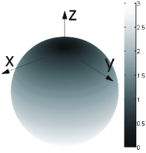
Figure 1: Scattering directivity pattern (absolute values) for an incident plane wave propagating along the $-z$-direction exciting a moving particle with the polarizabilities satisfying $\alpha_{\text{ee}}=\frac{1}{\eta_{0}^{2}}\alpha_{\text{mm}}$ (or an omega particle with ${-\alpha_{\text{ee}}-\frac{2}{\eta_{0}}\alpha+\frac{1}{\eta_{0}^{2}}\alpha_{\text{mm}}=0}$).

III-B2 Zero Forward Scattering

Similarly, we can derive conditions for zero forward scattering for these two classes of uniaxial particles. Again, zero forward scattering at oblique incidence is not possible as (27) and (28) are not satisfied. For the axial incidence with $\mathbf{u}=\mathbf{u}_{r}=\pm\mathbf{u}_{z}$, the zero forward scattering condition (29) simplifies to

$$\alpha_{\text{ee}}=-\frac{1}{\eta_{0}^{2}}\alpha_{\text{mm}}\quad\mbox{and arbitrary}\,\,\alpha$$ (44)

for an omega particle and

$$-\alpha_{\text{ee}}\pm\frac{2}{\eta_{0}}\alpha-\frac{1}{\eta_{0}^{2}}\alpha_{\text{mm}}=0$$ (45)

for a moving particle. The other zero forward scattering condition (30) vanishes for both particles. Here we should remember that the polarizabilities in (44) and (45) are complex numbers due to scattering losses. Thus, the condition for an omega particle cannot be realized, at least with a conventional passive uniaxial omega particle (realized, for example, as two orthogonal $\Omega$-shaped pieces of metal wire), because the imaginary parts of both polarizabilities have the same sign. Interestingly, the relation between the electric and magnetic polarizabilities (44) is the same condition that was derived for an electrically small isotropic magnetodielectric spherical particle in [3]. In that paper, the condition is given as $\epsilon_{r}=(4-\mu_{r})/(2\mu_{r}+1)$. This reduces to our condition as the normalized electric and magnetic polarizabilities are $\alpha_{\text{ee}}=(\epsilon_{r}-1)/(\epsilon_{r}+2)$ and $\alpha_{\text{mm}}=(\mu_{r}-1)/(\mu_{r}+2)$ for a small magnetodielectric spherical particle. Our result shows that this condition holds also for bi-anisotropic particles with omega coupling for arbitrary values of the coupling coefficient. As discussed above, the zero forward scattering conditions derived here can be satisfied only approximately with passive particles, in harmony with the optical theorem. For the special case of simple isotropic particles this issue was discussed in [5, 10].

Noticeably for a moving particle, we get different solutions for different incidence directions, similar to the omega particle case for zero backscattering. Again, the induced dipole moments are the same for both particles when the corresponding zero forward scattering conditions are satisfied. The dipole moments are non-zero meaning that there still can exist scattering in other directions.

If we enforce the zero forward scattering conditions (44) for an omega particle or (45) for a moving particle, the radiation vector for the axial incidence ($\mathbf{u}=\pm\mathbf{u}_{z}$) and an arbitrary scattering direction $\mathbf{u}_{r}$ has the form

$$\mathbf{F}_{\text{scat}}=(\alpha_{\text{ee}}\mp\alpha/\eta_{0})[(\mathbf{u}_{r}\times\overline{\overline{I}}_{\text{t}})\mp\overline{\overline{J}}_{\text{t}}]\cdot\mathbf{E}_{\text{inc}}.$$ (46)

It can be observed that this radiation vector has a form similar to (43) with only the sign of the $\overline{\overline{J}}_{\text{t}}$–term changed. Therefore, the scattering directivity pattern is also the same as the one shown in Fig. 1 albeit flipped so that there is now no scattering in the forward direction. Also, the polarization of the scattered field is linear as before.

III-B3 Zero Total Scattering

In the case of the omega particle, the zero total scattering conditions (31)–(34) simplify to

$$\alpha_{\text{ee}}=\pm\frac{1}{\eta_{0}}\alpha=-\frac{1}{\eta_{0}^{2}}\alpha_{\text{mm}}$$ (47)

which, again, cannot be fulfilled with a conventional passive omega particle, since the imaginary parts of $\alpha_{\text{ee}}$ and $\alpha_{\text{mm}}$ of passive particles have the same sign and they cannot be zero if particles receive and scatter power. In the case of a moving particle, we get

$$\alpha_{\text{ee}}=\pm\frac{1}{\eta_{0}}\alpha=\frac{1}{\eta_{0}^{2}}\alpha_{\text{mm}}.$$ (48)

which can be in principle satisfied, giving zero induced dipole moments. It is interesting to note that these conditions are the same as the conditions for the “optimal” bi-anisotropic particles whose energy in a given external field is maximized or minimized [29]. Also, if we satisfy zero total scattering conditions (47) or (48) for one axial propagation direction, a plane wave propagating in the opposite direction scatters from the particle, but the forward scattering amplitude in the case of an omega particle or the backscattering amplitude in the case of a moving particle is zero, because the zero forward scattering condition, (44), or the zero backscattering condition, (42), is satisfied for both propagation directions. As it was shown earlier that zero forward scattering with non-zero total scattering requires an active particle, this also implies that an invisible omega particle has to be active whereas an invisible moving particle does not have to be.

III-C Uniaxial Chiral Particle and Uniaxial Tellegen Particle

Next, we consider uniaxial chiral particles and uniaxial Tellegen particles oriented along the $z$-axis, with the polarizabilities of the form

$$\left\{\begin{array}[]{l}\displaystyle\overline{\overline{\alpha}}_{\text{ee}}=\alpha_{\text{ee}}\overline{\overline{I}}_{\text{t}}\vspace*{.2cm}\\ \displaystyle\overline{\overline{\alpha}}_{\text{mm}}=\alpha_{\text{mm}}\overline{\overline{I}}_{\text{t}}\vspace*{.2cm}\\ \displaystyle\overline{\overline{\alpha}}_{\text{em}}=\alpha_{\text{em}}\overline{\overline{I}}_{\text{t}}\vspace*{.2cm}\\ \displaystyle\overline{\overline{\alpha}}_{\text{me}}=\alpha_{\text{me}}\overline{\overline{I}}_{\text{t}},\end{array}\right.$$ (49)

that is, only the symmetric parts of the general polarizability dyadics (17)–(20) are non-zero. Furthermore, we have

$$\overline{\overline{\alpha}}_{\text{em}}=\pm\overline{\overline{\alpha}}_{\text{me}}=\alpha\overline{\overline{I}}_{\text{t}},$$ (50)

where ($+$) corresponds to a Tellegen particle and ($-$) to a chiral particle.

III-C1 Zero Backscattering

Based on (24) and (25), the zero backscattering condition for a chiral particle assuming axial incidence ($\mathbf{u}=\pm\mathbf{u}_{z}$) reads:

$$\alpha_{\text{ee}}=\frac{1}{\eta_{0}^{2}}\alpha_{\text{mm}}\quad\mbox{and arbitrary}\,\,\alpha.$$ (51)

As the condition $\overline{\overline{\alpha}}_{\text{em}}=-\overline{\overline{\alpha}}_{\text{me}}$ as well as the rotational symmetry condition are satisfied by definition for the chiral particle, we can conclude that the result is in agreement with the earlier results of [22, 24]. Also, as (22) and (23) are not satisfied, zero backscattering is only possible for the axial incidence. The radiation vector for the axial incidence ($\mathbf{u}=\pm\mathbf{u}_{z}$) when the zero backscattering condition is satisfied has the form

$$\mathbf{F}_{\text{scat}}=[\alpha_{\text{ee}}((\mathbf{u}_{r}\times\overline{\overline{I}}_{\text{t}})\pm\overline{\overline{J}}_{\text{t}})+\frac{\alpha}{\eta_{0}}(-\overline{\overline{I}}_{\text{t}}\pm(\mathbf{u}_{r}\times\overline{\overline{J}}_{\text{t}})]\cdot\mathbf{E}_{\text{inc}}.$$ (52)

In this case, the scattered wave excited by a linearly polarized plane wave is, in general case, elliptically polarized. The axial ratio of the scattered wave depends on the values of polarizabilities $\alpha_{\text{ee}}$ and $\alpha$. Because the zero backscattering condition does not include the field coupling coefficient $\alpha$, the axial ratio of the scattered field can be tuned by choosing the value of the chirality parameter.

As (25) has no solution for a Tellegen particle (except with $\alpha=0$), zero backscattering from a Tellegen particle excited by a linearly polarized plane wave is not possible.

III-C2 Zero Forward Scattering

Similarly, we can analyze conditions for zero forward scattering. In this case, equations (29)–(30) reduce for a Tellegen particle to

$$\alpha_{\text{ee}}=-\frac{1}{\eta_{0}^{2}}\alpha_{\text{mm}}\quad\mbox{and arbitrary}\,\,\alpha,$$ (53)

which is the same condition that we got for omega particles. Again, as (27) and (28) are not satisfied for a Tellegen particle, zero forward scattering is only possible for the axial incidence. In the Tellegen particle case, the radiation vector for the axial incidence ($\mathbf{u}=\pm\mathbf{u}_{z}$) when the zero forward scattering condition is satisfied has the form

$$\mathbf{F}_{\text{scat}}=[\alpha_{\text{ee}}((\mathbf{u}_{r}\times\overline{\overline{I}}_{\text{t}})\mp\overline{\overline{J}}_{\text{t}})+\frac{\alpha}{\eta_{0}}(\overline{\overline{I}}_{\text{t}}\pm(\mathbf{u}_{r}\times\overline{\overline{J}}_{\text{t}})]\cdot\mathbf{E}_{\text{inc}}.$$ (54)

Once more, the scattering directivity pattern is the same as shown in Fig. 1 (in this case corresponding to a wave propagating along the $+z$-direction) and the scattered wave is elliptically polarized. Also in this case we note that the polarization can be tuned by adjusting the field coupling coefficient, because (53) holds independently of the value of $\alpha$. As (30) has no solution for a chiral particle (except $\alpha=0$), zero forward scattering is not possible in this case.

TABLE II: Conditions for zero backscattering, zero forward scattering, and zero total scattering (if available), the axial ratio of the scattered wave when the corresponding condition is met (axial incidence) and the passivity/activity of the required particle. The top sign corresponds to the incident wave propagating along the $+z$-direction and the bottom sign along $-z$-direction. The incident plane wave is linearly polarized. $AR$ indicates the values of the axial ratio of the scattered field, where $AR=0$ corresponds to linear polarization.

	Chiral particle	Omega particle	Tellegen particle	Moving particle
backscattering Zero	$\alpha_{\text{ee}}=1/\eta_{0}^{2}\alpha_{\text{mm}}$ $-1\leq AR\leq 1$ passive	$-\alpha_{\text{ee}}\pm\frac{2}{\eta_{0}}\alpha+\frac{1}{\eta_{0}^{2}}\alpha_{\text{mm}}=0$ $AR=0$ passive		$\alpha_{\text{ee}}=1/\eta_{0}^{2}\alpha_{\text{mm}}$ $AR=0$ passive
scattering Zero forward		$\alpha_{\text{ee}}=-1/\eta_{0}^{2}\alpha_{\text{mm}}$ $AR=0$ active	$\alpha_{\text{ee}}=-1/\eta_{0}^{2}\alpha_{\text{mm}}$ $-1\leq AR\leq 1$ active	$-\alpha_{\text{ee}}\pm\frac{2}{\eta_{0}}\alpha-\frac{1}{\eta_{0}^{2}}\alpha_{\text{mm}}=0$ $AR=0$ active (unless also $\alpha_{\text{ee}}=1/\eta_{0}^{2}\alpha_{\text{mm}}$)
scattering Zero total		$\alpha_{\text{ee}}=\pm 1/\eta_{0}\alpha=-1/\eta_{0}^{2}\alpha_{\text{mm}}$ $AR=0$ active		$\alpha_{\text{ee}}=\pm 1/\eta_{0}\alpha=1/\eta_{0}^{2}\alpha_{\text{mm}}$ $AR=0$ passive

IV Simulation Results

In this section, we will demonstrate how zero backscattering and zero forward scattering conditions can be realized in practice with actual particles. We will use Ansys HFSS software to simulate the scattering of an incident linearly polarized plane wave from two reciprocal particles, one corresponding to zero backscattering (chiral particle) and the other one to zero forward scattering (omega particle). The material of the particles in this model is perfect electric conductor (PEC).

It is well known that a uniaxial particle with zero backscattering can be realized as two short dipole antennas connected to orthogonally oriented small loop antennas as long as the dipole and loop dimensions are chosen so that the particle is balanced, i.e., the condition (51) is satisfied [22, 23, 24]. An example design operating at the frequency 1.8 GHz is shown in Fig. 2. The length of one dipole arm is 20 mm, the loop radius is 8.75 mm, the radius of the wire is 0.2 mm, and the separation between the dipole arms is 5 mm. The corresponding scattering directivity pattern is shown in Fig. 3(a). Clearly, the scattering to the backward direction is minimized. Also, the shape of the scattering directivity pattern is very close to the ideal pattern of Fig. 1 and the maximum directivity is close to the theoretical value of 3. The scattering directivity in the backward direction is 0.18. The corresponding axial ratio pattern (absolute values) is shown in Fig. 3(b). Ideally, we should expect the axial ratio of 1 (i.e., the scattered field should have circular polarization) for lossless balanced chiral particles, but due to unwanted coupling between the two elements the axial ratio in the forward direction is only 0.77. This could be increased by, e.g., increasing the separation between the dipole arms. However, this would negatively affect the scattering directivity pattern.

As mentioned earlier, particles with zero forward scattering cannot be realized with passive inclusions. However, we can create a zero forward scattering particle by adding an active element to a conventional metal omega particle (in our example, a canonical omega particle consisting of two orthogonal $\Omega$-shaped metal wires). To be precise, this can be achieved by placing a voltage-driven wire loop next to an omega particle. If the external voltage applied to the loop has the opposite direction to the incident electric field and the appropriate amplitude and phase, we can effectively change the sign of the magnetic polarizability $\alpha_{\text{mm}}$, thus fulfilling the required condition for zero forward scattering for an omega particle (44). An example design for such a particle, operating at 1.8 GHz, is shown in Fig. 4 and the corresponding scattering directivity pattern in Fig. 5(a). The dimensions are the same as for the chiral particle, except that the separation between the dipole arms (i.e., the width of the loop gap) is 2.8 mm. The distance between the two loops is 1 mm. In this case, the forward scattering is clearly minimized and the pattern has a similar shape to the ideal pattern of Fig. 1, although the maximum directivity is slightly below 3. The scattering directivity in the forward direction is as small as 2.3$\times 10^{-7}$. The corresponding axial ratio pattern (absolute values) is shown in Fig. 5(b). The axial ratio is 0 (i.e., the scattered wave has linear polarization) for almost all the scattering directions. It should be noted that in order to have a truly uniaxial particle, another identical element should be added, orthogonal to the existing one, similarly to the uniaxial chiral particle considered above. The second element has been left out in this case for clarity and because it is practically invisible to the linearly polarized incident field as it is defined here.

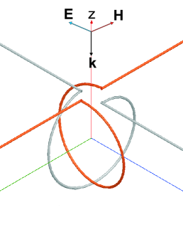
Figure 2: Uniaxial chiral particle showing zero backscattering at 1.8 GHz. The two elements are drawn with different colors only for clarity.

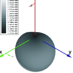
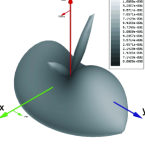
Figure 3: Scattering directivity pattern (a) and axial ratio pattern (b) for the chiral particle of Fig. 2 at 1.8 GHz (absolute values).

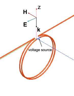
Figure 4: Active omega particle showing zero forward scattering at 1.8 GHz.

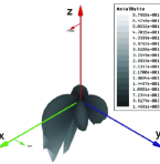
Figure 5: Scattering directivity pattern (a) and axial ratio pattern (b) for the active omega particle of Fig. 4 at 1.8 GHz (absolute values).

V Discussion and Conclusions

In this paper, scattering of a linearly polarized plane wave by small uniaxial bi-anisotropic particles has been studied. Firstly, the conditions for zero backward, forward, and total scattering conditions have been derived for a general uniaxial bi-anisotropic particle with all the polarizability dyadics having both symmetric and antisymmetric components. Zero backscattering as well as zero forward scattering for oblique incidence was shown to be possible only for certain special cases under the assumption that the axial polarizabilities are zero. For the axial incidence, requiring zero backscattering or zero forward scattering lead in both cases to two independent equations: one between the antisymmetric parts of the self-coupling polarizabilities and symmetric parts of the cross-coupling polarizabilities and one between the symmetric parts of the self-coupling polarizabilities and antisymmetric parts of the cross-coupling polarizabilities. Having zero total scattering from a particle, i.e., making the particle invisible, for one axial incidence direction was shown to be possible by balancing the particle response in particular ways. Secondly, four special cases of the general uniaxial bi-anisotropic particle (omega, moving particle, chiral, and Tellegen particles) have been analyzed and discussed in detail. The results show that zero backscattering property can be achieved for the axial excitation of a chiral or moving particle as long as the condition $\alpha_{\text{ee}}=\frac{1}{\eta_{0}^{2}}\alpha_{\text{mm}}$ is satisfied. A more complex condition, not satisfied by a “conventional” omega particle, of $-\alpha_{\text{ee}}\pm\frac{2}{\eta_{0}}\alpha+\frac{1}{\eta_{0}^{2}}\alpha_{\text{mm}}=0$ where $\pm$ corresponds to the opposite directions of the axially incident plane wave is required for an omega particle whereas zero backscattering is not possible for a Tellegen particle. The scattering pattern is the same in all the cases though the scattered wave has different polarizations. Zero forward scattering, on the other hand, can be achieved only for incident waves propagating along the particle axis with an omega or a Tellegen particle by fulfilling the condition $\alpha_{\text{ee}}=-\frac{1}{\eta_{0}^{2}}\alpha_{\text{mm}}$ or with a moving particle by fulfilling the condition $-\alpha_{\text{ee}}\pm\frac{2}{\eta_{0}}\alpha-\frac{1}{\eta_{0}^{2}}\alpha_{\text{mm}}=0$ where $\pm$ again correspond to the opposite directions of the axially propagating incident plane wave. Zero forward scattering condition is not possible to satisfy for a chiral particle. Moreover, the zero forward scattering condition can only be satisfied exactly with an active particle. The scattering pattern is the same for all the cases, but the polarization of the scattered wave differs. Zero total scattering for one incident direction along the particle axis can be achieved for a moving particle by satisfying $\alpha_{\text{ee}}=\pm 1/\eta_{0}\alpha=1/\eta_{0}^{2}\alpha_{\text{mm}}$ or for an omega particle by satisfying $\alpha_{\text{ee}}=\pm 1/\eta_{0}\alpha=-1/\eta_{0}^{2}\alpha_{\text{mm}}$ where the top sign corresponds to the positive propagation direction. When the illuminating plane wave travels in the opposite direction, the particle does not scatter in the backward direction in the case of an omega particle or the forward direction in the case of a moving particle, but does scatter in all the other directions.

The conditions for zero backscattering, zero forward scattering and zero total scattering when the scatterer is an omega particle, a moving particle, a chiral particle and a Tellegen particle are summarized in Table II. The axial ratio of the scattered wave when the corresponding scattering condition is met (the axial incidence with linear polarization) is also shown for each particle. Interestingly, we can see a kind of symmetry in the required conditions, as the conditions are the same for a chiral particle and a moving particle for zero backscattering as well as for an omega particle and a Tellegen particle for zero forward scattering. It should also be noted that all the results are in agreement with the zero backscattering conditions derived earlier in [1, 2, 24] and with the optical theorem.

Although in some of the studied cases shown in Table II the required particle can be easily realized as was demonstrated here numerically with zero-backscattering chiral particle and zero forward scattering omega particle, the practical design and in some cases even the feasibility of the required particle are as of yet unknown for many particle types, especially for the nonreciprocal ones. Conceptual discussions of possible structures exhibiting all the types of bi-anisotropic coupling can be found, e.g., in [19].

References

- [1] R.J. Wagner and P.J. Lynch, “Theorem on electromagnetic backscatter,” Phys. Rev., vol. 131, no. 1, pp. 21–23, 1963.
- [2] V. Weston, “Theory of absorbers in scattering,” IEEE Trans. Antennas Propag., vol. 11, no. 5, pp. 578–584, Sep. 1963.
- [3] M. Kerker, D.-S. Wang, and C.L. Giles, “Electromagnetic scattering by magnetic spheres,” J. Opt. Soc. Am., vol. 73, pp. 765–767, 1983.
- [4] B. Garcia-Camara, F. Gonzalez, F. Moreno, and J. M. Saiz, “Exception for the zero-forwardscattering theory,” J. Opt. Soc. Am. 1, vol. 25, pp. 2875–2878, 2008.
- [5] A. Alù and N. Engheta, “How does zero forward-scattering in magnetodielectric nanoparticles comply with the optical theorem?,” J. Nanophotonics, vol. 4, p. 041590, 2010.
- [6] A. Alù and N. Engheta, “Achieving transparency with plasmonic and metamaterial coatings,” Phys. Rev. E, vol. 72, p. 016623, Jul. 2005.
- [7] J.B. Pendry, D. Schurig, and D.R. Smith, “Controlling electromagnetic fields.” Science, vol. 312, pp. 1780–1782, May 2006.
- [8] U. Leonhardt, “Optical conformal mapping,” Science, vol. 312, pp. 1777–1780, Jun. 2006.
- [9] P. Alitalo and S.A. Tretyakov, “Broadband electromagnetic cloaking realized with transmission-line and waveguiding structures,” Proc. IEEE, vol. 99, pp. 1646–1659, 2010.
- [10] M. Nieto-Vesperinas, R. Gómez-Medina, and J.J. Saenz, “Angle-suppressed scattering and optical forces on submicrometer dielectric particles,” J. Opt. Soc. Am. A, vol. 28, no. 1, pp. 54–60, 2011.
- [11] R. Gómez-Medina, B. Garciá-Cámara, I. Suárez-Lacalle, F. González, F. Moreno, M. Nieto-Vesperinas, and J.J. Sáenz, “Electric and magnetic dipolar response of germanium nanospheres: interference effects, scattering anisotropy, and optical forces,” J. Nanophotonics, vol. 5, p. 053512, 2011.
- [12] A.E. Krasnok, A.E. Miroshnichenko, P.A. Belov, and Yu.S. Kivshar, “Huygens optical elements and Yagi-Uda nanoantennas based on dielectric nanoparticles,” JETP Letters, vol. 94, no. 8, pp. 593 -598, 2011.
- [13] D.S. Filonov, D.S. Filonov, A.E. Krasnok, A.P. Slobozhanyuk, P.V. Kapitanova, E.A. Nenasheva, Y.S. Kivshar, and P.A. Belov, “Experimental verification of the concept of all-dielectric nanoantennas,” Appl. Phys. Lett., vol. 100, p. 201113, 2012.
- [14] J.M. Geffrin, B. García-Cámara, R. Gómez-Medina, P. Albella, L.S. Froufe-Pérez, C. Eyraud, A. Litman, R. Vaillon, F. González, M. Nieto-Vesperinas, J.J. Sáenz, and F. Moreno, “Magnetic and electric coherence in forward- and back-scattered electromagnetic waves by a single dielectric subwavelength sphere,” Nature Communications, vol. 3, p. 1171, 2012.
- [15] M.J. Underhill and M.J. Blewett, “Undirectional tuned loop antennas using combined loop and dipole,” Proc. Eighth International Conference on HF Radio Systems and Techniques (IEE Conf. Publ. No. 474), pp. 37–41, Guildford, UK, July 2000.
- [16] S.R. Best, “Progress in the design and realization of an electrically small Huygens source,” Proc. IEEE International Workshop on Antenna Technology (iWAT 2010), pp. 1–4, Lisbon, Portugal, March 2010.
- [17] P. Jin P and R.W. Ziolkowski, “Metamaterial-inspired, electrically small Huygens sources,” IEEE Antennas and Wireless Propagation Letters, vol. 9, pp. 501–505, 2010.
- [18] T. Niemi, P. Alitalo, A.O. Karilainen, and S.A. Tretyakov, “Electrically small Huygens source antenna for linear polarisation,” IET Microwaves, Antennas & Propagation, vol. 6, no. 7, pp. 735–739, 2012.
- [19] A. Serdyukov, I. Semchenko, S. Tretyakov, and A. Sihvola, Electromagnetics of Bi-anisotropic Materials, Theory and Applications. Amsterdam, The Netherlands: Gordon and Breach, 2001.
- [20] P.L.E. Uslenghi, “Scattering by an impedance sphere coated with a chiral layer,” Electromagnetics, vol. 10, pp. 201–211, 1990.
- [21] P.L.E. Uslenghi, “Three theorems on zero backscattering,” IEEE Trans. Antennas Propag., vol. 44, no. 2, pp. 269–270, 1996.
- [22] A.O. Karilainen and S.A. Tretyakov, “Isotropic chiral objects with zero backscattering,” IEEE Trans. Antennas Propag., vol. 60, no. 9, pp. 4449–4452, 2012.
- [23] A.O. Karilainen and S. Tretyakov, “Circularly polarized receiving antenna incorporating two helices to achieve low backscattering,” IEEE Trans. Antennas Propagation, vol. 60, no. 7, pp. 3471–3475, 2012.
- [24] I.V. Lindell, A. Sihvola, P. Ylä-Oijala, and H. Wallén, “Zero backscattering from self-dual objects of finite size,” IEEE Trans. Antennas Propag., vol. 57, no. 9, pp. 2725–2731, Sep. 2009.
- [25] A. Sihvola, H. Wallén, P. Ylä-Oijala, M. Taskinen, H. Kettunen, and I.V. Lindell, “Scattering by DB spheres,” IEEE Antennas Wireless Propag. Lett., vol. 8, pp. 542–545, 2009.
- [26] P.A. Belov, S.I. Maslovski, K.R. Simovski, and S.A. Tretyakov, “A condition imposed on the electromagnetic polarizability of a bianisotropic scatterer,” Technical Physics Letters, vol. 29, no. 9, pp. 718–720, 2003.
- [27] C.T. Tai, Dyadic Green’s Functions in Electromagnetic Theory. Scranton, PA: Intext, 1971.
- [28] S.A. Tretyakov, A.H. Sihvola, A.A. Sochava, and C.R. Simovski, “Magnetoelectric interactions in bi-anisotropic media,” Journal of Electromagnetic Waves and Applications, vol. 12, no. 4, pp. 481–497, 1998.
- [29] S.A. Tretyakov, “The optimal material for interactions with linearly-polarized electromagnetic waves,” Proc. of the Fourth International Congress on Advanced Electromagnetic Materials in Microwaves and Optics (Metamaterials’2010), pp. 65–67, Karlsruhe, Germany, September 13-18, 2010.