Nonlinear response of quantum cascade structures

Abstract

The gain spectrum of a terahertz quantum cascade laser is analyzed by a non equilibrium Green’s functions approach. Higher harmonics of the response function were retrievable, providing a way to approach nonlinear phenomena in quantum cascade lasers theoretically. Gain is simulated under operation conditions and results are presented both for linear response and strong laser fields. An iterative way of reconstructing the field strength inside the laser cavity at lasing conditions is described using a measured value of the level of the losses of the studied system. Comparison with recent experimental data from time-domain-spectroscopy indicates that the experimental situation is beyond linear response.

Possible coherent radiation in the terahertz range has been a very strong motivation for research in the field of Terahertz Quantum Cascade LasersKöhler et al. (2002); Williams (2007) (THz-QCLs), which would enable a wide range of applications such as imagingDarmo et al. (2004) and spectroscopyHübers et al. (2006). However compact devices operating over cryogenic temperatures are a practical requirement for applications and currently the most promising designs are based on resonant phonon extraction Williams et al. (2003), achieving operating temperatures up to $\sim$ 200 K.Fathololoumi et al. (2012)

The key physical quantity in any QCL is the gain which describes the amplification of the optical field in the heterostructure material. In recent years this quantity has been measured in detail in Time-Domain-Spectroscopy (TDS) experimentsKröll et al. (2007); Burghoff et al. (2011) where THz-QCLs are probed by ultra short pulses providing information on both phase and amplitude of the transmitted pulse, whereafter the gain spectrum is reconstructed by a Fourier transform. The pulse is made as strong as possible in order to get a good signal to noise ratio but it is not known how the system dynamics are affected by such a measurement. The simulation of THz QCLs relies on a consistent treatment of tunneling and scattering, either by hybrid density matrix/rate equation schemes Callebaut and Hu (2005); Kumar and Hu (2009); Terazzi and Faist (2010); Dupont, Fathololoumi, and Liu (2010); Bhattacharya, Chan, and Hu (2012) or more evolved Non Equilibrium Green’s Function (NEGF) theory Lee et al. (2006); Schmielau and Pereira (2009); Kubis et al. (2009); Haldaś and, Kolek, and Tralle (2011). Here we present an extension of our NEGF schemeWacker, Nelander, and Weber (2009) towards the treatment of high intensities inside the QCL, going beyond linear response to an external electromagnetic field.

In this article we consider a time-dependent electric field $F(t)=F_{\rm dc}+F_{\rm ac}\cos(\Omega t)$ in the cavity, which reflects both the applied bias ($F_{\rm dc}$) and the electric component ($F_{\rm ac}$) of a monochromatic field of angular frequency $\Omega$ in the cavity. Going beyond linear response, this requires the solution of the time-dependent Kadanoff-Baym equation for the lesser and retarded Green’s functions, $G^{<}_{\alpha\beta}({\bf k},t_{1},t_{2})$ and $G^{\rm ret}_{\alpha\beta}({\bf k},t_{1},t_{2})$, respectively Haug and Jauho (1996). Here $\alpha,\beta$ denote the states in growth direction and ${\bf k}$ the in-plane momentum. The periodicity in time allows for a Fourier decomposition of the Green’s functions

$$G({\bf k};t_{1},t_{2})=\frac{1}{2\pi}\int{\rm d}E\sum_{h}\,{\rm e}^{-{\rm i}E(t_{1}-t_{2})/\hbar}G_{h}({\bf k},E){\rm e}^{-{\rm i}h\Omega t_{1}}$$ (1)

and similarly for the self-energies. This provides a set of equations for the Green’s functions for given self-energies $\Sigma_{\alpha\beta,h}({\bf k},E)$, which are defined analogously. This procedure follows essentially the concepts outlined in Ref. Brandes, 1997 and details will be given elsewhere. Here the terms with $h=0$ correspond to the stationary transport considered before Lee et al. (2006), while the higher order terms take into account the ac field. For the fields considered in this manuscript we used $h=-2,-1,0,1,2$, while checking that increasing $|h|$ did not change the results (generally higher values of $|h|$ are required with increasing ratios ${\rm e}F_{\rm ac}d/\hbar\Omega$, where $d$ is the period of the QCL structure). Relations to observables are made through the $h=0$ and $h=1$ components although the higher orders effect the lower ones implicitly. The Green’s functions allow for a determination of the current, where $G^{<}_{\alpha\beta\,h}({\bf k},E)$ provides the dc current for $h=0$ and the ac current with frequency $\Omega$ for $h=1$. Dividing the latter by $F_{\rm ac}$ provides the conductivity, directly related to the gain coefficient.

Here we consider the sample studied in Ref. Burghoff et al., 2011 as shown in Fig. 1(a). In Fig. 1(b) we show the current-bias relation, calculated by our model, together with experimental data. The original experimental data refer to the bias $U$ along the entire heterostructure, containing 175 periods of length $d$ as well as contact regions, where additional bias drops. In a similar experimentBurghoff et al. (2012) a voltage drop of around 3.0 V as well as a 5$\Omega$ series resistance were assumed for the data analysis. Here, we use a voltage drop of 3.8 V in the contacts for converting the experimental bias to $eF_{\rm dc}d$ as displayed in Fig. 1(b) and Fig. 3(b).

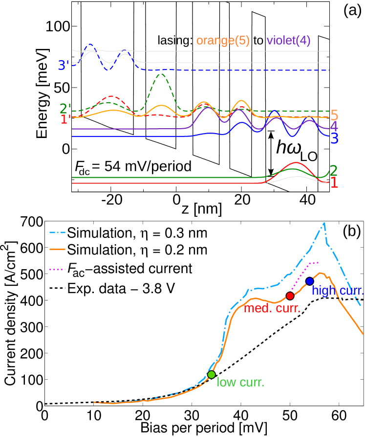
Figure 1: (Color online) (a) QCL structure considered with the main states contributing to its operation and (b) calculated current-bias relation for $\eta=0.2$ nm (solid) and $\eta=0.3$ nm (dotted-dashed) together with experimental data of Ref. Burghoff et al., 2011 (dashed). The shift in current at simulated operating conditions (dotted) is discussed later. The marked points at different current densities are analyzed in Fig. 2.

Fig. 1(b) displays simulations with different interface roughness scattering parameters in order to calibrate one of the parameters used, namely the average (RMS) of the roughness height $\eta$. This enters in the matrix element for the interface roughness scattering self energyLee and Wacker (2002) together with the typical size $\lambda=10$ nm of the roughness layers. According to Fig. 1(b) it is clear that a lower value of $\eta$ suppresses the current flow, and regarded as a fit parameter $\eta=0.20$ nm is a better value. All subsequent simulations where carried out with $\eta=0.20$ nm and a lattice temperature of 77 K entering the occupation of the phonon modes. The experimental heat-sink temperature was $\approx 33$ K Burghoff et al. (2011), but the lattice temperature for resonant phonon extraction THz-QCLs is typically higherVitiello et al. (2005) due to heating effects.

We note that for both simulations the main peak as well as the low-bias behavior are in good agreement with the experimental data. In contrast, for bias drops per period of about 40-45 mV, we observe a spurious extra peak due to tunneling between state 1 and state 3 of the next neighboring period. Such extra peaks for long-range tunneling have been observed in our model for other THz-structures as well, and we currently attribute them to the lack of electron-electron scattering processes.

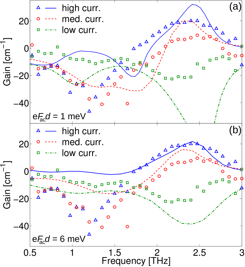
Figure 2: (Color online) Gain spectrum at different operation conditions for small ${\rm e}F_{\rm ac}d=1$ meV (a) and larger ${\rm e}F_{\rm ac}d=6$ meV (b) ac field strength. Open symbols are experimental data, and lines are simulated data. Green (dotted-dashed) corresponds to simulations at 34 mV/period, red (dashed) to 50 mV/period and blue (solid) to 54 mV/period. The experimental currents were 63, 319 and 403 A/cm² for the low, medium and high current respectively.

Fig. 2 shows the calculated gain spectra (lines) for three different dc biases, as depicted in Fig. 1(b), both for low (a) and high (b) ac field strength. For comparison, we display the experimental data from Ref. Burghoff et al., 2011 in both parts. The low current point ( $\square$/-$\cdot$-) is considered to be at the bias where state 1’ and 4 become aligned and electrons start to tunnel through the system as those levels are at resonance. Here we are far below threshold and mainly absorption is seen at the laser frequency of 2.2 THz, as state 4 – the lower laser state – is populated, while 5 is still mostly empty. This is changed as current is increased and we approach the medium current point ( $\circ$/- -). This is taken where the system is almost at, but still below the threshold current. Here the states 1’ and 5 start to align, creating population inversion at the laser frequency. At operating conditions, where the third and last point ( $\triangle$/-) at high current is taken, gain is above the level of the lossesBurghoff et al. (2011) of 18 cm^-1 and can now sustain lasing as the population inversion is at its maximum.

The simulations at low and high ac field strength shown in Fig. 2 differ drastically, but the general picture is that around the laser frequency, large losses at low current develop into gain as bias is raised, as observed by Refs. Martl et al., 2011; Burghoff et al., 2011. At a more detailed level, the low ac field strength simulations exhibit stronger features which are not reflected in the experimental data. At higher ac field strength however, the overall agreement becomes better, mainly due to a redistribution of carriers (bleaching). However, the strong absorption feature around 1.2 THz for medium and high current density in the experimental data does not appear in the simulations, for which we do not have any explanation. The better agreement of experimental data with high ac field, indicates that the experimental conditions are beyond linear response.

Here it is important to address the fundamental differences between experiment and simulation. In the simulations, a monochromatic ac field is applied and the gain spectrum is constructed frequency by frequency. In the experimental case, the situation is quite different. A pulse, containing all frequencies within the bandwidth (typically 3 THzKröll et al. (2007)) is sent into the sample, and the way this pulse has changed by passing through the structure determines the gain spectrum. Compared to the simulations, where we only measure at the frequency where we excite, this is the opposite, as all frequencies are subject to excitations and all frequencies are also measured. Therefore, our modeling can only be seen as approximate. In addition, the experimental data is the difference of measurements between the unbiased QCL and the QCL at the chosen measuring bias. This way the background is effectively subtracted. If the structure exhibits less losses at some point than it does at zero bias, this is measured as gain. In the simulations however, we only extract the gain from the conductivity extracted from the $h=1$ component of the Green’s functions, as we do not have to take losses into account and thus only look at the intrinsic gain spectra. Simulations at very low bias, i.e. the off-state, show absorption peaks at 0.9 THz and 2.7 THz, which could explain corresponding features in the experimental gain spectra.

We have demonstrated, that the response varies significantly with the ac field strength. Thus it is important to question whether the ac field strengths used in the simulations are comparable to their experimental counterpart. In order for the effects of high ac field strengths shown in Fig. 2(b) to be of any relevance, the power coupled into the QCL structure during the experimental measurements must be sufficient. Addressing this question, consider the experimental situation governing the in-coupling of lightBurghoff et al. (2011): A pumping femtosecond pulse of 125 mW hits the emitter section of the same QCL as described in Fig. 1. The pulse generates a photocurrent giving an electric field transient that is coupled across an air distance of 4 $\mu$m into the QCL section of interest. Our value ${\rm e}F_{\rm ac}d=6$ meV corresponds to a power of 40 mW in the cavity, which requires an extremely efficient conversion in the emitter and good coupling between the structures. It is far from clear, whether the probing field can reach these intensities. Strong ac fields at lasing conditions would be capable of generating these effects, but this would then only contribute above threshold current.

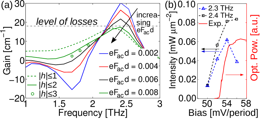
Figure 3: (Color online) (a) Gain spectra at a bias of 54 mV/period at different ac field strengths. (b) Calculated intensities in the waveguide (dashed) and corresponding experimental data (full line).

In a working laser, the gain will clamp at the level of the losses, as the population inversion will stabilize around the configuration where the inversion lost to the optical field will be balanced by the injector efficiency. This happens at different intensities for different bias points, and using this fact the intensity at gain clamping and thus the power in the QCL can be reconstructed theoretically. One can use the level of the losses measured in Ref. Burghoff et al., 2011 in order to iteratively calculate the intensity at operating conditions. Fig. 3(a) shows gain spectra at a bias of 54 mV/period that have been simulated at various ac-field strengths. It is clear from Fig. 3 that higher ac field strengths effectively lower both gain and absorption, and give rise to gain bleaching. For all bias points above threshold simulations were carried out at different ac field strengths in order to see which ones gave gain matching the level of the losses at 18 cm^-1. The corresponding intensities were then extracted and are shown in Fig. 3(b). For the maximum intensity of 0.08 mW/$\mu$m² the wave guide area of 800 $\mu$m² provides a power of 64 mW inside the QCL. This seems reasonable taking into account that only a part is coupled out through the mirror.

To show the importance of including higher orders of the Fourier decomposed Green’s function in Eq. (1), simulations with $|h|\leq 1$ only and also $|h|\leq 3$ is shown in Fig. 3(a) for ${\rm e}F_{\rm ac}d=8$ meV which is the highest ac-field used. $|h|\leq 1$ (dashed) shows a clear deviation from the $|h|\leq 2$ case (full line) while the simulations with $|h|\leq 3$ confirm the quality of our $|h|\leq 2$ calculations for ${\rm e}F_{\rm ac}d\lesssim/\hbar\Omega$.

The $F_{\rm ac}$-assisted current at the intensities shown in Fig. 3(b) is displayed as a dotted line in Fig. 1(b). It increases proportional to the intensity compared to the non-lasing current. Thus when lasing sets in, we see a kink in the current, just as in the experimental data of Fig. 1(b) at 53 mV per period. As the calculated kink appears somewhat stronger, our calculated lasing intensities could be a little bit too high. This may be related to the fact, that the experimental lasing frequency of 2.2 THz is not precisely at the peak of the gain spectrum.

In conclusion, we have simulated gain under operation by including higher orders of the Fourier decomposed Green’s function in order to include nonlinear effects. We have found a way to calculate the power of the laser using an experimental value of the level of the losses and by iteratively matching the gain to that level and then extract the intensity of such a configuration. It has also been shown that gain bleaches under high intensity conditions and that this might be a non negligible effect in THz-TDS measurements.