A stopping criterion for Markov chains when generating independent random graphs

Abstract

Markov chains are convenient means of generating realizations of networks with a given (joint or otherwise) degree distribution, since they simply require a procedure for rewiring edges. The major challenge is to find the right number of steps to run such a chain, so that we generate truly independent samples. Theoretical bounds for mixing times of these Markov chains are too large to be practically useful. Practitioners have no useful guide for choosing the length, and tend to pick numbers fairly arbitrarily. We give a principled mathematical argument showing that it suffices for the length to be proportional to the number of desired number of edges. We also prescribe a method for choosing this proportionality constant. We run a series of experiments showing that the distributions of common graph properties converge in this time, providing empirical evidence for our claims.

I Introduction

Graphs are a common topological representation across a variety of scientific fields. They are used when relations between a large number of entities have to be specified in a succinct manner. Chemical reactions, molecules, social networks (both physical and online) and the electric grid are some common examples. In many cases, we may have partial information about the graph, requiring generation of many graphical realizations consistent with the (partial) characterization. Such situations arise in case of large online social networks (of which only a small part can be sampled tractably) or where the data simply cannot be collected e.g., the web of human sexual relations (which only allows the estimation of the degree distribution). In other cases, privacy concerns can prevent the distribution of a graph for experimentation and or study, e.g., networks of email communications, critical infrastructure nets, etc. This gives rise to the problem of constructing “sanitized” proxies, that preserve only some properties of the original graph. Thus, being able to generate independent graphs conditioned on an incomplete set of graphical measurements is essential for many applications.

Many graph generation methods aim to preserve the salient features of graphs 12sk3a ; 12pf4a ; 55hv1a ; 62hs1a ; 96wp2a ; kronecker ; Aiello00 ; Chung2 ; 12gk3a . For statistical analysis, we need algorithms that can generate uniformly random instances from the space of graphs with a specified feature. There has been significant work on random graph generation with a given degree distribution (DD), which specifies the number of vertices with a given degree. In ktv , the problem of generating a graph with a given degree distribution was reduced to a prefect matching problem, which can be used to generate random instances by employing results in sampling perfect matchings JeSiVi04 ; Br86 . Alternatively, sequential sampling methods were investigated in BlDi11 ; BaKiSa10 . These methods can be compute intensive, and in practice, Markov chains (MC) are widely used due to their simplicity and flexibility. The MC is started using a graph that honors the specified graphical characteristics, and uses a procedure that can “rewire” a graph, to create ensembles of graphs with the same degree distribution. Taylor 81tr1a showed that edge-swaps could modify a graph while preserving its DD. Kannan et al ktv analyzed the mixing time of such a MC, whereas Gkantsidis GkantsidisMMZ03 devised a MC scheme that avoids self loops. In StPi12 , Stanton and Pinar used an MC to generate an ensemble of graphs using a rewiring scheme that preserved the joint degree distribution (JDD), which specifies the number of edges between vertices of specified degrees. Stanton and Pinar also empirically analyzed the mixing of the MC using the binary “time-series” traced out by the appearance/disappearance of edges between two labeled nodes, as the MC executed its random walk in the space of graphs. They showed that the autocorrelation of the time-series decayed to zero, a necessary condition for the MC to converge to its stationary distribution Sokal .

Graph rewiring schemes that preserve DD or JDD are simple (and fast) and MC chains driving them are easy to construct. However, successive graphs generated by the MC are only slightly different and the MC has to proceed for a large number of steps $N$ before the initial graph is “forgotten.” The mixing time estimates in ktv take the form of upper bounds and of $O(|E|^{6})$, where $|E|$ is the number of edges in a graph. Even for small graphs with 1000 edges, the bound is intractable. In practice, $N$ is chosen arbitrarily. Failure to mix completely leads to the generation of correlated samples and any results derived from them are erroneous. While the method in StPi12 demonstrated the use of autocorrelation to establish mixing, it is an a posteriori test which provides no a priori guidance regarding the length of the MC chain. Further, the method requires a small, user-specified threshold, below which the time-series autocorrelation is deemed zero.

In this paper, we construct analytical models that estimate $N$. These models track the evolution of the binary “time-series” formed by the edges of labeled graphs generated by the MC. We test the model under conditions where the DD or the JDD is held constant. In Sec. II, the model is used to derive an expression for the mixing time based on when the binary time-series begins to resemble independent draws from a distribution. The models predict that the mixing time is proportional to $|E|$, the number of edges in the graph. The model holds true for a “representative” edge and exploits the constancy of DD (or JDD) in arriving at its prediction. The model is tested with real graphs in Sec. III. In Sec. IV, we develop a data-driven method, that assumes neither a constant DD (or JDD) nor a representative edge, to investigate the independence of the edge time-series. We use this test to verify the assumptions made when developing mixing time expressions in Sec. II. We determine the fraction of the edges for which the model prediction of $N$ is an underestimate, and the consequences of the lack of stationarity on the ensemble of graphs sampled in this manner.

II Theoretical analysis

The goal of this paper is to provide a mathematically principled argument for running a MC ${\rm O(|E|)}$ steps to generate independent graphs with $|E|$ edges. The constant hidden in the big-Oh depends on the desired accuracy. The graphs so generated may have a prescribed DD or a JDD; we find that a MC on graphs with a prescribed DD mixes slightly easier than those where the JDD is preserved. Our empirical results show that ${\rm 5|E|}$ – ${\rm 30|E|}$ steps are sufficient for mixing these MCs. We provide a mathematical justification for this observation.

Consider a MC on the space of graphs and two labeled vertices $u$ and $v$. Under certain circumstances, the existence of an edge $(u,v)$ can also be described by a Markov chain. Thus we model the behavior of the MC on the space of graphs in terms of a set of coupled 2-state Markov chains, each representing edge behavior. We develop the transition matrix for the (edge) MC, which is exact for DD-preserving experiments, but heuristically derived for MCs with prescribed JDDs. We prove an ${\rm O(|E|)}$ mixing time for these 2-state Markov chains. This ensures that that after ${\rm O(|E|)}$ MC steps, each edge behaves as if it comes out of independent draws. While this is not sufficient for complete mixing, it is a necessary condition.

These mathematical theorems will be empirically validated in the next section, but we give a quick preview of the method. Starting from a real graph, we run a MC (driving a DD- or JDD-preserving rewiring scheme) for $\ell$ steps, to create a new, nominally independent graph. This is repeated $M$ times to create an ensemble of graphs. We plot the distribution of some common graphical quantity (e.g., the number of triangles in each graph) constructed from the ensemble. This is repeated for different values of $\ell$ till the plots converge. We find that $\ell\sim{\rm 10|E|}$. When $\ell\sim{\rm|E|}$, the MC is far from convergence.

Below, we review the rewiring schemes used in the paper. This is followed by derivations of the models of mixing under DD and JDD preservation.

II.1 A review of rewiring schemes

Consider an undirected graph $G=(V,E)$, where $|V|=n$, the number of vertices in the graph, and $|E|=m$, the number of edges. The degree distribution of the graph is given by the vector $\mathbf{f}$, where $\mathbf{f}(d)$ is the number of vertices of degree $d$. The joint degree distribution is an $n\times n$ matrix $\mathbf{J}$, where $\mathbf{J}(i,j)$ is the number of edges incident between vertices of degree $i$ and degree $j$. We use $d_{v}$ to denote the degree of vertex $v$.

Figure 1: The DD-preserving swapping operation described in Sec. II.1.

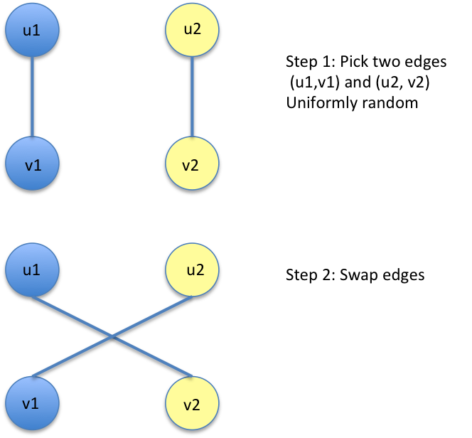
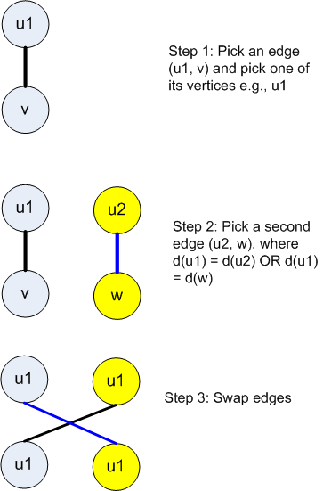
In this paper, we use the greedy, JDD-preserving rewiring procedure by Stanton and Pinar in StPi12 . This is analogous to the degree distribution preserving chain ktv ; GkantsidisMMZ03 , illustrated in Fig 1. The JDD-preserving rewiring procedure is shown in Fig 2. The procedure does not guard against parallel edges or self-loops, but the MC itself can be slightly modified to ensure that these artifacts do not occur StPi12 ; GkantsidisMMZ03 . We also maintain lists of nodes and edges indexed by their degree, so that for a given degree $d$, we can locate a uniform random edge that is incident on a degree-$d$ node. The steps in the rewiring scheme are:

• Pick an endpoint uniformly at random. This is done by picking a random edge and choosing one of its endpoints with equal probability. Let this vertex be $u_{1}$. We then choose a uniform random neighbor $v$ of $u_{1}$, to get edge $(u_{1},v)$.

• Pick uniformly at random another vertex $u_{2}$ such that $d_{u_{1}}=d_{u_{2}}$, and choose a uniform random neighbor $w$ incident to $u_{2}$. This gives the second edge.

• Swap the edges $(u_{1},v)$ and $(u_{2},w)$ to create $(u_{1},w)$ and $(u_{2},v)$.

Details of the rewiring scheme and discussions of the ergodicity, mixing of a MC driving such a rewiring scheme can be found in StPi12 . A pictorial description is in Fig. 2.

Figure 2: The JDD-preserving swapping operation described in Sec. II.1.

II.2 Modeling mixing when degree distribution is preserved

Consider a MC ${\cal M}$ that generates graphs with a prescribed degree distribution. Consider two labeled vertices $u$ and $v$, with degrees $d_{u}$ and $d_{v}$. We will show that the appearance/disappearance of $(u,v)$ in ${\cal M}$ can also be described by a Markov chain.

Claim 1.

The transition matrix of the Markov chain for the edge $(u,v)$ is given by

$${\bm{\mathbf{{T}}}}(d_{u},d_{v}) = \left(\begin{array}[]{cc}1-\alpha(d_{u},d_{v})&\alpha(d_{u},d_{v})\\ \beta(d_{u},d_{v})&1-\beta(d_{u},d_{v})\end{array}\right)$$ (3)

where $\alpha(d_{u},d_{v})=\frac{d_{u}d_{v}}{2m^{2}}$, $\beta(d_{u},d_{v})=1-(1-1/m)^{2}$, and the first index in $T$ is state $0$ (no edge).

Proof.

Assume that the edge $(u,v)$ does not initially exist. We analyze the probability of it appearing after one step. Let $e$ and $e^{\prime}$ be the two edges chosen by the rewiring algorithm. $(u,v)$ will appear if $u$ is the first endpoints of $e$ and $v$ is the last endpoint of $e^{\prime}$ (or vice versa). This leads to four possible cases. Consider the case when both the vertices are the first endpoints of $e$ and $e^{\prime}$. The probability of this event is $d_{u}/2m\times d_{v}/2m=d_{u}d_{v}/4m^{2}$. The other case is symmetric and so $\alpha(d_{u},d_{v})=d_{u}d_{v}/2m^{2}$.

Suppose that $(u,v)$ does exist but is removed during the Markov transition. This occurs if $(u,v)$ is either $e$ or $e^{\prime}$. The probability of this event is $\beta_{(}d_{u},d_{v})=1-(1-1/m)^{2}$. Note that the values of $\alpha$ and $\beta$ so derived are completely independent of the structure of the rest of the graph, and so the transition probabilities in Eq. 3 satisfy the Markov property. ∎

II.3 Modeling mixing when joint degree distribution is preserved

We consider a pair of labeled vertices $(u,v)$ and model the appearance/disappearance of the edge during a Markov transition. For convenience, we will assume that $\mathbf{f}(d_{u})$ and $\mathbf{f}(d_{v})$ are both strictly greater than $1$. The proofs can be extended to these cases as well. (Observe that when $\mathbf{f}(d_{u})=\mathbf{f}(d_{v})$, the edge $(u,v)$ is always present because the JDD is preserved.)

Claim 2.

Assume edge $(u,v)$ is present and is removed using the transition. The probability of this event is

$$\beta(d_{u},d_{v})=\frac{1}{m}+\frac{\mathbf{f}(d_{u})-1}{2m\mathbf{f}(d_{u})}+\frac{\mathbf{f}(d_{v})-1}{2m\mathbf{f}(d_{v})}$$ (4)

Proof.

We follow the JDD-preserving swapping procedure described in Sec. II.1. Let $e$ and $e^{\prime}$ be the two edges chosen for swapping. If $(u,v)$ is $e$, it will definitely be swapped. The probability of the chosen edge being $(u,v)$ is $1/m$.

The other alternative is that $(u,v)$ is $e^{\prime}$. This can happen only if the first endpoint chosen has degree $d_{u}$ (or $d_{v}$) and then $(u,v)$ is chosen. Consider the first case. The total number of endpoints on degree $d_{u}$ vertices (excluding $u$) is $(\mathbf{f}(d_{u})-1)d_{u}$. The probability that $e$ is chosen is the probability that $u$ is chosen as the second endpoint, and then $(u,v)$ is chosen. This is equal to $1/(\mathbf{f}(d_{u})\times d_{u})$. The total probability is

$$\frac{(\mathbf{f}(d_{u})-1)d_{u}}{2m}\times\frac{1}{\mathbf{f}(d_{u})d_{u}}=\frac{(\mathbf{f}(d_{u})-1)d_{u}}{2m\mathbf{f}(d_{u})d_{u}}=\frac{\mathbf{f}(d_{u})-1}{2m\mathbf{f}(d_{u})}$$

Symmetrically, the randomly chosen endpoint could have had degree $d_{v}$. So the total probability of choosing $e^{\prime}=(u,v)$ is

$$\frac{\mathbf{f}(d_{u})-1}{2m\mathbf{f}(d_{u})}+\frac{\mathbf{f}(d_{v})-1}{2m\mathbf{f}(d_{v})}$$

and the probability of $(u,v)$ being removed is

$$\beta(d_{u},d_{v})=\frac{1}{m}+\frac{\mathbf{f}(d_{u})-1}{2m\mathbf{f}(d_{u})}+\frac{\mathbf{f}(d_{v})-1}{2m\mathbf{f}(d_{v})}.$$

∎

This expression has certain ramifications. Since the JDD is preserved (and by implication, $\mathbf{f}(d)$), the probability of edge removal does not vary as the Markov chain proceeds. This satisfies the Markov property and $\beta$ depends only on $u$ and $v$ i.e., it is independent of the rest of the graph.

Consider the probability $\alpha$ of $(u,v)$ appearing. This is not Markovian, as it depends on the structure of the graph. However, this dependence is weak, and we can obtain a Markovian approximation using a simple heuristic.

Consider the number of edges ${\bm{\mathbf{{J}}}}(d,d_{v})$ between vertices of degree $d_{v}$ and an arbitrary $d$. The expected number of such edges incident on a degree $d_{v}$ vertex is ${\bm{\mathbf{{J}}}}(d,d_{v})/\mathbf{f}(d_{v})$. The number of edges between a vertex $v$ and degree $d$ vertices depends on the graphical structure; however, we will approximate it with the expected value ${\bm{\mathbf{{J}}}}(d,d_{v})/\mathbf{f}(d_{v})$.

Claim 3.

If $(u,v)$ is not present at a stage in the Markov chain, the probability $\alpha$ that it appears in the next step is given by

$$\alpha(d_{u},d_{v})=\frac{2{\bm{\mathbf{{J}}}}(d_{u},d_{v})}{m\mathbf{f}(d_{u})\mathbf{f}(d_{v})}$$ (5)

Proof.

As before, let the two edges chosen by the algorithm be $e$ and $e^{\prime}$, in that order. The edge $(u,v)$ is swapped in when either of the four following situations happens. Vertex $u$ is the first (resp. second) endpoint of $e$ and $v$ is the second (resp. first) endpoint of $e^{\prime}$. Or, vertex $u$ is the first (resp. second) endpoint of $e^{\prime}$ and $v$ is the second (resp. first) endpoint of $e$.

$u$ is the first endpoint of $e$ and $v$ is the second endpoint of $e^{\prime}$ (or vice versa).

Consider the following sequence of events. First, $u$ is chosen as an endpoint (and we get edge $e$). Then, we choose a vertex $u^{\prime}$ (who is a neighbor of $v$) whose degree is the same as $u$. Finally, we select edge $e^{\prime}=(u^{\prime},v)$. Swapping will lead to edge $(u,v)$. The probability of the first event is $d_{u}/2m$. The probability of the second event depends the number of neighbors of degree $d_{u}$ incident to $v$. Alternately, this is the number of edges connecting $v$ to degree $d_{u}$ vertices. Clearly, this depends on the graph structure, but our approximation of this quantity is ${\bm{\mathbf{{J}}}}(d_{u},d_{v})/\mathbf{f}(d_{v})$.

So, the second probability is ${\bm{\mathbf{{J}}}}(d_{u},d_{v})/(\mathbf{f}(d_{v})\mathbf{f}(d_{u}))$ (because there are $\mathbf{f}(d_{u})$ neighbors of degree $d_{u}$, of which ${\bm{\mathbf{{J}}}}(d_{u},d_{v})/\mathbf{f}(d_{v})$ are neighbors of $v$). The last probability is $1/d_{u}$. The total probability is

$$\frac{d_{u}}{2m}\times\frac{{\bm{\mathbf{{J}}}}(d_{u},d_{v})}{\mathbf{f}(d_{u})\mathbf{f}(d_{v})}\times\frac{1}{d_{u}}=\frac{{\bm{\mathbf{{J}}}}(d_{u},d_{v})}{2m\mathbf{f}(d_{u})\mathbf{f}(d_{v})}$$

Now consider the second case. First, $v^{\prime}$ (a neighbor of $u$ whose degree is $d_{v}$) is chosen as an endpoint. Then, $u$ is chosen as the neighbor of $v^{\prime}$, so $e=(u,v^{\prime})$. Then, $v$ is chosen as the first endpoint of the second edge $e^{\prime}$. Swapping will again lead to edge $(u,v)$. The first probability is approximated by $\mathbf{J}(d_{u},d_{v})/(\mathbf{f}(d_{u})\mathbf{f}(d_{v}))$. The second probability is $1/d_{v}$, and the last is $d_{v}/2m$. The probability comes out to be the same as earlier.

By symmetry, we get the probabilities of the other cases by switching the roles of $u$ and $v$, yielding the same expression. ∎

II.4 Estimating the mixing time

Having developed expressions for $\alpha$ and $\beta$ in Eq. 3, under the assumption of prescribed DD (Sec. II.2) and JDD (Sec. II.3), we use the Markov transition matrix to estimate the number of steps $N$ to achieve a stationary distribution, conditional on a tolerance $\epsilon$.

Claim 4.

Choose $N$ as follows. Let the final distribution after running ${\cal M}_{u,v}$ for $N$ steps be ${\mathbf{p}}$. Then $\|{\mathbf{p}}-\bm{\pi}_{u,v}\|<\varepsilon$.

$$N=\begin{cases}(m/2)\ln(1/\varepsilon)&\mathrm{DD\;preserving\;\;MCs}\\ m\ln(1/\varepsilon)&\mathrm{JDD\;preserving\;\;MCs}\end{cases}$$

The distribution $\bm{\pi}_{u,v}$ is the probability of existence/absence of edge $(u,v)$ once ${\cal M}$ has converged. This implies that after $N=m\ln(1/\varepsilon)$ we are very close to the converged distribution of all edges, irrespective of the degrees of their terminating vertices.

Proof.

${\bm{\mathbf{{T}}}}$ has two eigenvalues, $1$ and $1-(\alpha(d_{u},d_{v})+\beta(d_{u},d_{v}))$. Let the corresponding unit eigenvectors be ${\mathbf{e}}_{1}$ and ${\mathbf{e}}_{2}$. For notational convenience we will refer to $\alpha(d_{u},d_{v})$ and $\beta(d_{u},d_{v})$ as $\alpha$ and $\beta$. Since $\alpha+\beta>0$, the eigenvectors form a basis. We represent the initial state of the MC as ${\mathbf{v}}=c_{1}{\mathbf{e}}_{1}+c_{2}{\mathbf{e}}_{2}$. After $N$ applications of the transition matrix, the distribution of the Markov chain’s state is

$${\mathbf{p}} = {\bm{\mathbf{{T}}}}^{N}{\mathbf{v}}=c_{1}{\bm{\mathbf{{T}}}}^{N}{\mathbf{e}}_{1}+c_{2}{\bm{\mathbf{{T}}}}^{N}{\mathbf{e}}_{2}$$ (6)

$$= c_{1}{\mathbf{e}}_{1}+c_{2}\left(1-(\alpha+\beta)\right)^{N}{\mathbf{e}}_{2}.$$

Since $(1-(\alpha+\beta))<1$, the second term decays with $N$, and the stationary distribution asymptotically approaches $c_{1}{\mathbf{e}}_{1}$. The 2-norm of the decaying term (the error incurred when we stop at finite $N$) can be bounded for

$$N=\ln{(1/\epsilon)}/(\alpha+\beta)$$

in the following manner

$$\|{\mathbf{p}}-\bm{\pi}_{u,v}\| = \|(1-\gamma)^{N}c_{2}{\mathbf{e}}_{2}\|_{2}\leq(1-\gamma)^{\ln(1/\varepsilon)/\gamma}c_{2}\|{\mathbf{e}}_{2}\|_{2}$$

$$\leq \exp(-\ln(1/\varepsilon))=\varepsilon$$

where we have used $\gamma=(\alpha+\beta)$ and

$$N = \frac{m}{2}\ln{\frac{1}{\epsilon}}\geq\frac{1}{\gamma}\ln{\frac{1}{\epsilon}},\mbox{\hskip 8.53581pt for DD-preserving MC and}$$

$$N = m\ln{\frac{1}{\epsilon}}\geq\frac{1}{\gamma}\ln{\frac{1}{\epsilon}},\mbox{\hskip 8.53581pt for JDD-preserving MC.}$$ (7)

The key observation is $\gamma\geq 2/m$ for DD-preserving MC (see values of $\alpha$ and $\beta$ in Sec. II.2) and $\gamma\geq 1/m$ for a JDD-preserving MC (see Sec. II.3). ∎

III Tests with real graphs

In this section we perform empirical studies to find a suitable value of $\epsilon$, i.e., one which can be used to generate samples of graphs which are statistically indistinguishable from those generated by a smaller $\epsilon$. We discriminate graphs using certain graphical metrics.

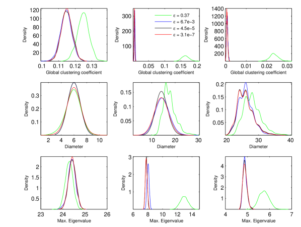
We run the MC with the DD-preserving rewiring scheme for $N$ steps before saving the resultant graph. We start the MC using 4 real graphs - the neural network of C. Elegans celegans1 (referred to as “C. Elegans”), the power grid of the Western states of US celegans1 (called “Power”), co-authorship graph of network science researchers adjnoun (referred to as “Netscience”) and a 75,000 vertex graph of the social network at Epinions.com 03ra3a (“soc-Epinions1”). Their details are in Table 1. The first three were obtained from newman_graphs while the fourth was downloaded from snap . All the graphs were converted to undirected graphs by symmetrizing the edges.

We use $N=\{0.5,2.5,5,7.5\}|E|$ corresponding to $\epsilon=\{0.37,6.7\times 10^{-3},4.5\times 10^{-5},3.06\times 10^{-7}\}$. 1000 graphs are generated in this manner, starting with the real graphs in Table 1. Thereafter, we calculate the global clustering coefficient (three times the ratio of the number of triangles to wedges in a graph)BaWe00 , the diameter, and the maximum eigenvalue of the Laplacian matrix of the graph Me94 for each of members of the ensemble of 1000 graphs. In Fig. 3, we plot these distributions for three of the four graphs in Table 1. We clearly see that for $\epsilon=0.37$ i.e., $N=0.5|E|$, the distributions for all graphical metrics are quite different from the distributions obtained with $N>|E|$. The red and black curves, corresponding to $N=5|E|$ and $N=7.5|E|$ are mostly indistinguishable indicating that the MC has converged to its stationary distributions. We will henceforth proceed with $\epsilon=4.5\times 10^{-5}$, achieved with $N=5|E|$ when the DD is preserved during the MC sampling.

Table 1: Characteristics of the graphs used in this paper. $(|V|,|E|)$ are the numbers of vertices and edges in the graph and G-R diagnostic is the Gelman-Rubin diagnostic.

Graph name	$(|V|,|E|)$	G-R diagnostic
C. Elegans	(297, 4296)	1.05
Netscience	(1461, 5484)	1.02
Power	(4941, 13188)	1.006
soc-Epinions1	(75879, 405740)	1.06

Figure 3: Plots of the distributions of the global clustering coefficient, the diameter, and the maximum eigenvalue of the graph Laplacian for “C. Elegans” (left), “Netscience” (middle) and “Power” (right), evaluated after $0.5|E|,2.5|E|,5|E|$ and $7.5|E|$ iterations of the Markov chain (green, blue, black and red lines respectively). The corresponding values of $\epsilon$ are in the legend. We see that the distributions converge at $\epsilon\sim 1e-5$. In these runs, the DD was held constant across all graphical samples.

We now turn our attention to the case when the JDD is preserved during MC sampling. We repeat the same sampling procedure as above, but with the JDD-preserving rewiring scheme being driven by the Markov chain. We choose the same sequence of $\epsilon$, corresponding to $N=\{1,5,10,15\}|E|$, per Eq. 7. The distributions of global clustering coefficients, graph diameter and maximum eigenvalue of the graph Laplacian are in Fig. 4. Again, it is clear that the distribution (for any of the graphical metrics) is far from convergence for $\epsilon=0.37$ but indistinguishable for the other values of $\epsilon$. In particular, the red and black plots lie on top of each other in most of the subfigures, indicating that $N=10|E|$ ($\epsilon=4.5\times 10^{-5}$) is generally sufficient to drive the MC to its stationary distribution, as characterized by the aforementioned graphical parameters.

Figure 4: Plots of the distributions of the global clustering coefficient, the diameter, and the maximum eigenvalue of the graph Laplacian for “C. Elegans” (left), “Netscience” (middle) and “Power” (right), evaluated after $|E|,5|E|,10|E|$ and $15|E|$ iterations of the Markov chain (green, blue, black and red lines respectively). The corresponding values of $\epsilon$ are in the legend. We see that the distributions converge at $\epsilon\sim 1e-5$. In these runs, the JDD was held constant across all graphical samples.

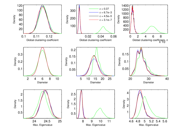
In summary, a tolerance of $\epsilon=4.5\times 10^{-5}$ provides converged/stationary distributions of global clustering coefficient, graph diameter and maximum eigenvalue of the graph Laplacian. This corresponds to running the MC on the space of graphs for $N=5|E|$ steps when DD is preserved and for $N=10|E|$ steps when JDD is preserved. These results provide an empirical proof that the models in Sec. II.2 and Sec. II.3 provide a good a priori estimate of the steps to run a MC to obtain stationary results.

IV Verification of model assumptions

In this section, we check our assumption that a MC on the space of graphs can be approximated by coupled 2-state Markov chains. We also devise a test to ensure that the MC does not converge to a local mode in the distribution of graphs. This can occur in case of multimodal distributions.

IV.1 Verifying edge-by-edge convergence

The equation for $N$ (Eq. 7) is based on a heuristic and has to be verified. Further, the equation is strictly valid for an edge and it is unlikely that after $N$ steps of the MC, all the edges have decorrelated and converged to their stationary distribution. The residual number of correlated edges have to be identified and their impact on graphical properties quantified.

Consider the behavior of an arbitrary edge (between labeled vertices) during a long walk executed by a MC on the space of graphs. During this walk, the edge appears and disappears, thus describing a binary time-series $\{Z_{t}\}$. If the MC on the space of graphs reaches a stationary distribution in ${\rm O(|E|)}$ steps, then thinning the binary time-series by a factor of ${\rm O(|E|)}$ should result in a time-series that resembles independent draws of zeros and ones. We develop a nonparametric test of independence for such time-series. This method exploits Sokal’s observation that if an MC reaches a stationary distribution, the samples it draws are uncorrelated i.e., the autocorrelation is small Sokal . It is general and does not depend on the preservation of DD or JDD in the graphs. While this test has been in existence for some time 92rl2a ; 96ra1a , it is not well known in the network generation literature.

Assume that the time-series $\{Z_{t}\}$ is very long i.e., it takes $K\gg N$ steps. The time-series will be correlated as observed in StPi12 . Consider too, a $k$-thinned chain $\{Z^{k}_{t}\}$, obtained by retaining every $k^{th}$ member of $\{Z_{t}\}$. The thinned chain will have a far smaller autocorrelation and upon further thinning will begin to resemble independent draws from a distribution. If Eq. 7 is correct, $k=N$ should yield a time-series that resembles independent draws more than a first-order Markov process. This forms the basis of our test of independence. We fit models of two processes, independence and first-order Markov, to the data and compute the log-likelihood. The “goodness” of model fit is determined by computing the Bayesian Information Criterion (BIC). This paper is the first application of this technique to graphs, though it has been used in other contexts.

Let $x_{ij}$ be the number of $(i,j),i,j\in(0,1)$ transitions in the $k-$thinned chain $\{Z^{k}_{t}\}$. The $x_{ij}$ are used to populate $X$, a $2\times 2$ contingency table. The table entries are normalized by the length of the $k$-thinned chain ($K/k-1$) to provide us with the empirical probabilities $p_{ij}$ of an $(i,j)$ transition in $\{Z^{k}_{t}\}$. Let $\widehat{p_{ij}}$ and $\widehat{x_{ij}}=(K/k-1)\widehat{p_{ij}}$ be the predictions of expected values of the table entries provided by a model. Then the goodness-of-fit of the model can be provided by a likelihood ratio statistic (called the $G^{2}$-statistic; Chapter 4.2 in 07bfh3a ) and a Bayesian Information Criterion (BIC) score:

$$G^{2} = -2\sum_{i=0}^{i=1}\sum_{i=0}^{i=1}x_{ij}\log\left(\frac{\widehat{x_{ij}}}{x_{ij}}\right),$$

$$BIC = G^{2}+q\log\left(\frac{K}{k}-1\right),$$ (8)

where $q$ is the number of parameters in the model used to fit the table data. Log-linear models are generally used to model tabular data (Chapter 2.2.3 in 07bfh3a ). The log-linear models’ predictions for table entries generated by independent sampling and a first-order Markov process are

$$\log(p_{ij}^{(I)}) = u^{(I)}+u^{(I)}_{1,(i)}+u^{(I)}_{2,(j)}\mbox{\hskip 5.69054pt and \hskip 5.69054pt}$$

$$\log(p_{ij}^{(M)}) = u^{(M)}+u^{(M)}_{1,(i)}+u^{(M)}_{2,(j)}+u^{(M)}_{12,(ij)},$$ (9)

where superscripts $I,M$ indicate an independent and a Markov process respectively. The maximum likelihood estimates (MLE) of the parameters ($u^{(W)}_{b,(c)}$) are available in closed form in literature (Chapters 2.2.3 and 3.1.2 in 07bfh3a ) and we reproduce them below:

$$\widehat{x_{ij}^{I}}=\frac{(x_{i+})(x_{+j})}{x_{++}}\mbox{\hskip 5.69054pt and \hskip 5.69054pt}\widehat{x_{ij}^{M}}=x_{ij},$$ (10)

where $x_{i+}$ and $x_{+j}$ are the sums of the table entries in row $i$ and column $j$ respectively. $x_{++}$ is the sum of all entries (i.e., $K/k-1$, the number of transitions observed in $\{Z^{k}_{t}\}$, or the total number of data points). We compare the fits of the two models thus:

$$\Delta BIC = BIC^{(I)}-BIC^{(M)}$$

$$= -2\sum_{i=0}^{i=1}\sum_{i=0}^{i=1}x_{ij}\log\left(\frac{\widehat{x_{ij}^{(I)}}}{x_{ij}}\right)-\log\left(\frac{K}{k}-1\right).$$

Above, we have substituted $\widehat{x_{ij}^{(M)}}=x_{ij}$ and the fact that the log-linear model for a Markov process has one more parameter than the independent sampler model. Large BIC values indicate a bad fit. A negative $\Delta BIC$ indicates that an independent model fits better than a Markov model.

This test is applied as follows. We construct a thinned binary time-series $\{Z^{k}_{t}\}$ for $k=|E|$ for each of the edges. The $\Delta BIC$ is computed and edges with negative $\Delta BIC$ are deemed to have become independent after $k$ steps of the Markov chain. The test is repeated with a higher $k$ till all the edges are deemed to have become independent. A C++ implementation of this test, using a binary time-series as input, is available at papersoftware .

However, a difficulty appears at this point. We see that the accuracy of the log-linear models in Eq. 9 and 10 depend on the length of the chain being tested i.e., if the chain is too short, the ratio of likelihoods and the BIC will be wrongly calculated. Thus, before we populate the contingency table, we ensure that the edge time-series is long enough.

Consider an edge time-series obtained from the $K$-step MC. One can empirically compute the edge-mean $\overline{Z_{t}}$ i.e., the probability of existence of the edge. An estimate of the same quantity can be obtained from a $k-$thinned version of the chain i.e., $\overline{Z^{k}_{t}}$. If the thinned time-series are sufficiently long, then the estimates of the edge mean, $\overline{Z^{k}_{t}}$, computed for different values of $k$, approximately describe a normal distribution, with mean $q$ (the edge mean) and a variance $\sigma^{2}$.

We wish to ensure that a $k$-thinned MC is sufficiently long, i.e., the empirical edge-mean $\overline{Z^{k}_{t}}$ can be estimated to lie inside $q\pm r$ with confidence $s$ i.e.$P(q-r\leq\overline{Z^{k}_{t}}<q+r)=s$, or

$$\left(\frac{r}{\Phi^{-1}\{0.5(1+s)\}}\right)^{2}=\sigma^{2}$$ (12)

where $\Phi$ is the cumulative distribution function for a standard normal distribution and $r$ is a tolerance on the empirical edge-mean calculated using a $k$-thinned MC.

Consider that thinning the $K$-step time-series by a factor $k^{\prime}$ renders it a first-order MC (see Appendix A on how this may be done). The contingency table entries (Eq. 10) then indicate the number (or proportions) of 0-1 and 1-0 transitions of the 2-state Markov chain model of the time-series. It is then trivial to compute the entries $\alpha$ and $\beta$ of the Markov transition matrix. If $n^{\prime}$ is the length of the $k^{\prime}$-thinned time-series, then the variance of the $\overline{Z^{k}_{t}}$, $\sigma^{2}$ can be written in terms of $\alpha,\beta$,

$$\sigma^{2}=\frac{\alpha\beta(2-\alpha-\beta)}{n^{\prime}(\alpha+\beta)^{3}}$$

and so, using Eq. 12,

$$n^{\prime}=\frac{\frac{\alpha\beta(2-\alpha-\beta)}{(\alpha+\beta)^{3}}}{\left(\frac{r}{\Phi^{-1}\{0.5(1+s)\}}\right)^{2}},$$ (13)

i.e., the $k^{\prime}$-thinned time-series must be at least $n^{\prime}$ in length to provide an estimate $\overline{Z^{k}_{t}}$ of $q$ (computed from the $K$-step time-series) within tolerance $r$ with the required confidence $s$. In this paper, we use $r=0.01$ and $s=0.95$.

We now apply this test to a Markov chain on graphs initiated with those mentioned in Table 1. In Fig. 5 we see the thinning factors required to render the $k$-thinned time-series $\{Z^{k}_{t}\}$ resemble independent draws from a distribution. In Fig. 5 (left) we see that thinning by $4|E|$ is sufficient to render $\{Z^{k}_{t}\}$ independent, for all three graphs tested, when the DD is preserved by the MC. In Fig. 5 (right) we see results for the JDD-preserving counterpart. It is clear that higher thinning factors are required for independence, but a thinning factor of $10|E|$ seems to be sufficient. Thus empirically, the factor-of-two difference in $N$, as predicted by the models in Eq. 7, and as seen empirically in Fig. 3 and Fig. 4, are corroborated by a separate test that does not assume DD or JDD preservation.

Figure 5: Fraction of edges testing independent, for “C. Elegans”, “Netscience” and “Power” for various values of the thinning factor $k$. Left: Results for the case when DD is preserved. We see that with a thinning factor of $k=4|E|$ all the edges have converged to their stationary distribution. Right: Results for the case when JDD was preserved. We see that $k=10|E|$ ensures that at least 95% of the edges become independent.

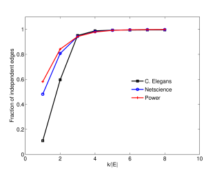
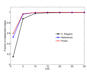
Convergence of distributions of global clustering coefficients, diameter and maximum eigenvalues do not automatically indicate that the time-series of all the edges in a graph resemble independent draws. This is clearly seen in Fig. 4 for the graph “Power” (bottom row). In Fig. 4, $N\sim 10|E|$ ($\epsilon=4.5\times 10^{-5}$) was sufficient to construct distributions that do not change appreciably for greater $N$. However, from Fig. 5, we see that about 2% of the edges are still not independent, but presumably close to being so, since about $15|E|$ steps of the MC result in all edges becoming independent.

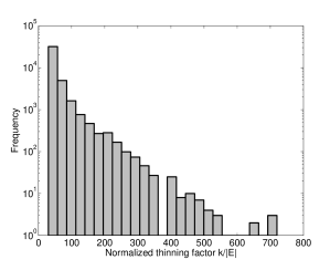
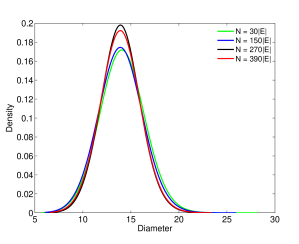
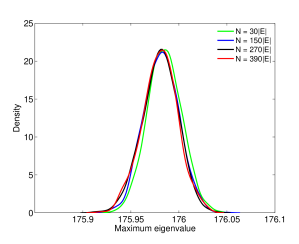
In order to check this issue, we performed a test with the soc-Epinions1 graph. We generate an ensemble of 1000 graphs using $N=30|E|$ and the method in Sec. II.3 i.e., where the JDD of the initial graph was preserved as samples were generated. We also run a long $K$-step MC ($K=21.6\times 10^{6}|E|$) and compute the thinning factor $k$ required to render each edge’s time-series similar to independent draws. Since the graph has 405,740 edges, the independence test was performed for only 10% of the edges, chosen randomly from the initial graph. In Fig. 6 we plot a histogram of $k/|E|$. We clearly see that while by $k=30|E|$ about 90% of the edges have become independent, there are quite a few “pathological” edges that are very far from becoming independent (one such edge becomes independent at $k=720|E|$). In Fig. 7 we plot the distributions for the diameter and the maximum eigenvalue for $N=30|E|,150|E|,270|E|$ and $390|E|$. We see that the two distributions, while not identical, do not change much. Thus distributions of the chosen metrics are robust (insensitive) to an ensemble which might contain graphs with a few “hard-to-converge” edges. Thus, if one is interested in generating proxy graphs where anonymity is critical (e.g. proxies of email traffic in an organization), an exhaustive, edge-by-edge checking of independence, using the method described above, may be necessary. On the other hand, when one only desires a collection of roughly independent graphs with a prescribed DD or JDD, the far simpler approach of Sec. II.2 or II.3 may suffice.

Figure 6: A histogram of $k/|E|$, where $k$ is the number of steps the MC has to take to render the time-series of a particular edge resemble independent draws, calculated for the soc-Epinions1 graph. We see that while $30|E|$ steps render about 90% of the edges independent, there are a few edges which are still very far from becoming independent.These results are for a case where the JDD was preserved.

Figure 7: Plots of the distribution of graph diameter (left) and maximum eigenvalue of the graph’s Laplacian (right) for $N=30|E|,150|E|,270|E|$ and $390|E|$, for the soc-Epinions1 graph (green, blue, black and red lines respectively). We see that distributions are very similar, even though, from Fig. 6, it is evident that a few edges are far from being independent. Thus these two graphical metrics are not very sensitive graphs that are almost, but not quite, independent. These results are for a case where the JDD was preserved.

IV.2 The Gelman-Rubin test for convergence of Markov chains

Finally we address the question whether the MC generating the ensemble of graphs is sampling from a particular mode of the distribution of graphs (in case the distribution is multimodal). This can, in principle, occur since the MC is always started from the same starting graph. Convergence to the stationary distribution (and not just to one mode) can be tested by starting the MC from an overdispersed set of points and checking whether the same distributions are realized, irrespective of the starting point. In our case, we will choose three points and perform this test only for the JDD-preserving case.

In order to generate a set of overdispersed starting graphs, we run a Markov chain for $N=10,000|E|$ steps, after initializing it with a real network. This serves as the second over-dispersed starting point for the MC and the initial condition for the third point (realized after another 10,000$|E|$ steps). Three concurrent MC are initialized with these graphs, and we calculate the Gelman-Rubin (G-R) diagnostic 92gr1a using the binary edge time-series. Values of the diagnostic between 1 and 1.1 indicate that the states of the concurrent Markov chain are not dependent on the starting location. We performed this test for all 4 graphs; the corresponding G-R diagnostics are tabulated in Table 1.

V Conclusions

We have developed a method for generating independent realizations of graphs which share a particular graphical property. In this paper, we have demonstrated the method in the case where (1) the degree distribution was preserved over all realizations and (2) where the joint degree distribution was held constant. The graphs are generated using a MC approach, which drives a graph “rewiring” scheme. The rewiring scheme is responsible for preserving the shared graphical properties when it generates a new graphical realization, from an old one. Our method involves running the Markov chain for $N$ steps before extracting a graph; the chain is run repeatedly to generate an ensemble of realizations, given an initial graph. We have developed models and closed form expressions for $N$ that allows a coupled 2-state Markov chain of an edge to converge to its stationary distribution. This is a necessary, but not sufficient, condition for the Markov chain on the space of graphs to “forget” the starting graph and generate an independent realization. We find that a Markov chain requires $5|E|-30|E|$ steps to mix fully, i.e., to provide converged distributions of graphical properties like the global clustering coefficient, graph diameter and maximum eigenvalues of the graph Laplacian. We find that the Markov chains that preserve the degree distribution are easier to mix than those where the joint degree distribution is held constant.

We verified our model (for $N$) by performing a test for the independence of the Markov chain described by any edge between two labeled vertices in the graph, as the Markov chain on the space of graphs executes its random walk. This test is not dependent on any heuristic or graphical properties. The test uses the time-series of occurrence/non-occurrence of an edge between labeled vertices, thins them by a factor of $N$, and fits it with a first-order Markov and an independent sampling model. The goodness of fit of the two models, determined by their individual BICs, is used to select between them. The Markov chain is considered mixed for any $N$ for which the independence sampling model is selected over the Markov model. We find that even for $N$ that provide converged distributions of the graphical properties above, a small fraction of the edges may still be significantly correlated (as determined by the independence test). The robustness of the graphical properties indicate that if fully independent graphical realizations are desired, the laborious process of testing each edge may be unavoidable.

Finally, we repeated our tests by starting parallel Markov chains from widely dispersed starting points and computing the Gelman-Rubin diagnostic for them. We find that the parallel chains converge to the same stationary distribution. This check was performed to ensure that our distributions of graphical properties was not being driven by the starting point of the Markov chain.

Apart from the theoretical results summarized above, we also provide an open-source C++ implementation of the non-parametric test, along with sample problems to illustrate its use papersoftware .

Appendix A

Here, we address how one may thin a long, $K$-step time-series so that the thinned chain resembles a first-order Markov process. It follows the arguments in Sec. IV.1. We consider a binary time-series and populate a $2\times 2\times 2$ contingency table of transitions that one might observe in a sequence of length three. The contingency table is fitted with log-linear models for second- and first-order Markov models (see Sec. 7.3.1 in 07bfh3a for second-order Markov models), and the $G^{2}$ statistic calculated along with the difference in the BICs arising from second-order and first-order Markov model fits.

Initially, the high-order Markov model fits to data better than the first-order model. However, as the $K$-step time-series is thinned, and the correlation decays, the fit of first-order model, vis-á-vis, the second-order model improves. At a particular thinning factor $k^{\prime}$ the first-order model fits better than the second order one (the difference in BICs favors the first-order model) and we obtain a first-order Markov chain.

In the software that we have released with this paper papersoftware , the C function mctest() checks the fit of a time-series to first- and second-order Markov chains, returning the ratio of likelihoods and the difference in the BICs of the two models. The C function indtest() does the same, but between a first-order Markov model and independent draws from a binary distribution. Both the functions construct the contigency table from the binary time-series supplied via the function arguments, and compute the expected values of the table entries (using log-linear models calibrated to table data). In contrast, the function mcest() estimates the transition probabilities $\alpha$ and $\beta$ from a binary time-series, being modeled as a first-order Markov process. Examples of the use of the tests (mctest and indtest) are illustrated in the software package associated with this paper (in ex01/). The use of all the functions, in a MC on graphs, is in ex02/.

References and Notes

- (1) W. Aiello, F. Chung, and L. Lu, A random graph model for power law graphs, Experimental Math, 10 (2000), pp. 53–66.
- (2) A. Barrat and M. Weigt, On the properties of small-world network models, The European Physical Journal B - Condensed Matter and Complex Systems, 13 (2000), pp. 547–560.
- (3) M. Bayati, J. H. Kim, and A. Saberi, A sequential algorithm for generating random graphs, Algorithmica, 58 (2010), pp. 860–910.
- (4) Y. M. Bishop, S. E. Fienberg, and P. W. Holland, Discrete multivariate analysis: Theory and practice, Springer-Verlag, New York, NY, 2007.
- (5) J. Blitzstein and P. Diaconis, A sequential importance sampling algorithm for generating random graphs with prescribed degrees, Internet Mathematics, 6 (2011), pp. 489–522.
- (6) A. Z. Broder, How hard is it to marry at random? (on the approximation of the permanent), in Proceedings of the eighteenth annual ACM symposium on Theory of computing, STOC ’86, New York, NY, USA, 1986, ACM, pp. 50–58.
- (7) F. R. K. Chung and L. Lu, The average distance in a random graph with given expected degrees, Internet Mathematics, 1 (2003).
- (8) A. Gelman and D. B. Rubin, Inference from iterative simulation using multiple sequences, Statistical Science, 7 (1992), pp. 457–472.
- (9) M. Gjoka, M. Kurant, and A. Markopoulou, 2.5K-Graphs: from Sampling to Generation, ArXiv e-prints, (2012).
- (10) C. Gkantsidis, M. Mihail, and E. W. Zegura, The Markov chain simulation method for generating connected power law random graphs, ALENEX, (2003), pp. 16–25.
- (11) S. L. Hakimi, On the realizability of a set of integers as degrees of the vertices of a simple graph, J. SIAM Appl. Math., 10 (1962), pp. 496–506.
- (12) V. Havel, A remark on the existence of finite graphs, C̆asopis. Pĕst. Mat., 80 (1995), pp. 477–480.
- (13) M. Jerrum, A. Sinclair, and E. Vigoda, A polynomial-time approximation algorithm for the permanent of a matrix with nonnegative entries, J. ACM, 51 (2004), pp. 671–697.
- (14) R. Kannan, P. Tetali, and S. Vempala, Simple Markov-chain algorithms for generating bipartite graphs and tournaments, Random Struct. Algorithms, 14 (1999), pp. 293–308.
- (15) J. Leskovec, D. Chakrabarti, J. Kleinberg, C. Faloutsos, and Z. Ghahramani, Kronecker graphs: An approach to modeling networks, Journal of Machine Learning Research (JMLR), 11 (2010), pp. 985–1042.
- (16) R. Merris, Laplacian matrices of graphs: a survey, Linear Algebra and its Applications, 197-198 (1994), pp. 143 – 176.
- (17) M. E. J. Newman, Prof. M. E. J. Newman’s collection of graphs at University of Michigan. http://www-personal.umich.edu/mejn/netdata/.
- (18) M. E. J. Newman, Finding community structure in networks using the eigenvectors of matrices, 036104, Phys. Rev. E, 74 (2006).
- (19) J. J. Pfeiffer, III, T. La Fond, S. Moreno, and J. Neville, Fast Generation of Large Scale Social Networks with Clustering, ArXiv e-prints, (2012).
- (20) A. Raftery and S. M. Lewis, Implementing MCMC, in Markov Chain Monte Carlo in Practice, W. R. Gilks, S. Richardson, and D. J. Spiegelhalter, eds., Chapman and Hall, 1996, pp. 115–130.
- (21) A. E. Raftery and S. M. Lewis, How many iterations in the Gibbs sampler?, in Bayesian Statistics, J. M. Bernardo, J. O. Berger, A. P. Dawid, and A. F. M. Smith, eds., vol. 4, Oxford University Press, 1992, pp. 765–766.
- (22) J. Ray, A. Pinar, and C. Safta, graphMC: A package for testing the independence of graphs. http://www.sandia.gov/apinar/graphMC/graphMC.html.
- (23) M. Richardson, R. Agrawal, and P. Domingos, Trust management for the semantic Web, in The Semantic Web - ISWC 2003, D. Fensel, K. Sycara, and J. Mylopoulos, eds., vol. 2870 of Lecture Notes in Computer Science, Springer Berlin / Heidelberg, 2003, pp. 351–368. 10.1007/978-3-540-39718-2_23.
- (24) C. Seshadhri, T. G. Kolda, and A. Pinar, Community structure and scale-free collections of Erdös-Rényi graphs, Phys. Rev. E, 85 (2012), p. 056109.
- (25) A. Sokal, Monte Carlo methods in statistical mechanics: Foundations and new algorithms, 1996.
- (26) Stanford Network Analysis Platform Collection of Graphs, The Epinions social network from the Stanford Network Analysis Platform collection. http://snap.stanford.edu/data/soc-Epinions1.html.
- (27) I. Stanton and A. Pinar, Constructing and sampling graphs with a prescribed joint degree distribution using Markov chains, ACM Journal of Experimental Algorithmics. to appear.
- (28) R. Taylor, Constrained switchings in graphs, in Combinatorial Mathematics VIII, K. McAvaney, ed., vol. 884 of Lecture Notes in Mathematics, Springer Berlin / Heidelberg, 1981, pp. 314–336. 10.1007/BFb0091828.
- (29) S. Wasserman and P. E. Pattison, Logit models and logistic regression for social networks: I. An introduction to Markov graphs and , Psychometrika, 61 (1996), pp. 401–425.
- (30) D. J. Watts and S. H. Strogatz, Collective dynamics of ’small-world’ networks, Nature, 393 (1998), pp. 440–442.