On U-Statistics and Compressed Sensing I: Non-Asymptotic Average-Case Analysis

Abstract

Hoeffding’s U-statistics model combinatorial-type matrix parameters (appearing in CS theory) in a natural way. This paper proposes using these statistics for analyzing random compressed sensing matrices, in the non-asymptotic regime (relevant to practice). The aim is to address certain pessimisms of “worst-case” restricted isometry analyses, as observed by both Blanchard & Dossal, et. al.

We show how U-statistics can obtain “average-case” analyses, by relating to statistical restricted isometry property (StRIP) type recovery guarantees. However unlike standard StRIP, random signal models are not required; the analysis here holds in the almost sure (probabilistic) sense. For Gaussian/bounded entry matrices, we show that both $\ell_{1}$-minimization and LASSO essentially require on the order of $k\cdot[\log((n-k)/u)+\sqrt{2(k/n)\log(n/k)}]$ measurements to respectively recover at least $1-5u$ fraction, and $1-4u$ fraction, of the signals. Noisy conditions are considered. Empirical evidence suggests our analysis to compare well to Donoho & Tanner’s recent large deviation bounds for $\ell_{0}/\ell_{1}$-equivalence, in the regime of block lengths $1000\sim 3000$ with high undersampling ($50\sim 150$ measurements); similar system sizes are found in recent CS implementation.

In this work, it is assumed throughout that matrix columns are independently sampled.

I Introduction

Compressed sensing (CS) analysis involves relatively recent results from random matrix theory [1], whereby recovery guarantees are framed in the context of matrix parameters known as restricted isometry constants. Other matrix parameters are also often studied in CS. Earlier work on sparse approximation considered a matrix parameter known as mutual coherence [2, 3, 4]. Fuchs’ work on Karush-Kuhn-Tucker (KKT) conditions for sparsity pattern recovery considered a parameter involving a matrix pseudoinverse [5], re-occurring in recent work [4, 6, 7]. Finally, the null-space property [8, 9, 10] is gaining recent popularity - being the parameter closest related to the fundamental compression limit dictated by Gel’fand widths. All above parameters share a similar feature, that is they are defined over subsets of a certain fixed size $k$. This combinatorial nature makes them difficult to evaluate, even for moderate block lengths $n$. Most CS work therefore involve some form of randomization to help the analysis.

While the celebrated $k\log(n/k)$ result was initially approached via asymptotics, e.g., [1, 11, 12, 13], implementations require finite block sizes. Hence, non-asymptotic analyses are more application relevant. In the same practical aspect, recent work deals with non-asymptotic analysis of deterministic CS matrices, see [14, 15, 4, 7]. On the other hand certain situations may not allow control over the sampling process, whereby the sampling may be inherently random, e.g., prediction of clinical outcomes of various tumors based on gene expressions [6]. Random sampling has certain desirable simplicity/efficiency features - see [16] on data acquisition in the distributed sensor setting. Also recent hardware implementations point out energy/complexity-cost benefits of implementing pseudo-random binary sequences [17, 18, 19]; these sequences mimic statistical behavior. Non-asymptotic analysis is particularly valuable, when random samples are costly to acquire. For example, each clinical trial could be expensive to conduct an excessive number of times. In the systems setting, the application could be running on a tight energy budget - whereby processing/communication costs depend on the number of samples acquired.

This work is inspired by the statistical notion of the restricted isometry property (StRIP), initially developed for deterministic CS analysis [14, 15]. The idea is to relax the analysis, by allowing sampling matrix parameters (that guarantee signal recovery) to be satisfied for a fraction of subsets. Our interest is in “average-case” notions in the context of randomized sampling, reason being that certain pessimisms of “worst-case” restricted isometry analyses have been observed in past works [13, 20, 21]. On the other hand in [22], Donoho & Tanner remarked on potential benefits of the above “average-case” notion, recently pursued in an adaptation of a previous asymptotic result [23]. In the multichannel setting, “average-case” notions are employed to make analysis more tractable [24, 25]. In [26] a simple “thresholding” algorithm is analyzed via an “average” coherence parameter. However the works in this respect are few, most random analyses are of the “worst-case” type, see [27, 12, 13, 21]. We investigate the unexplored, with the aim of providing new insights and obtaining new/improved results for the “average-case”.

Here we consider a random analysis tool that is well-suited to the CS context, yet seemingly left untouched in the literature. Our approach differs from that of deterministic matrices, where “average-case” analysis is typically made accessible via mutual coherence, see [14, 15, 18]. For random matrices, we propose an alternative approach via U-statistics, which do not require random signal models typically introduced in StRIP analysis, see [14, 26, 25]; here, the results are stated in the almost sure sense. U-statistics apply naturally to various kinds of non-asymptotic CS analyses, since they are designed for combinatorial-type parameters. Also, they have a natural “average-case” interpretation, which we apply to recent recovery guarantees that share the same “average-case” characteristic. Finally thanks to the wealth of U-statistical literature, the theory developed here is open to other extensions, e.g., in related work [28] we demonstrate how U-statistics may also perform “worst-case” analysis.

Contributions: “Average-case” analyses are developed based on U-statistics, which are i) empirically observed to have good potential for predicting CS recovery in non-asymptotic regimes, and ii) theoretically obtain measurement rates that incorporate a non-zero failure rate (similar to the $k\log(n/k)$ rate from “worst-case” analyses). We utilize a U-statistical large deviation concentration theorem, under the assumption that the matrix columns are independently sampled. The large deviation error bound holds almost surely (Theorem 1). No random signal model is needed, and the error is of the order $(n/k)^{-1}\log(n/k)$, whereby $k$ is the U-statistic kernel size (and $k$ also equals sparsity level). Gaussian/bounded entry matrices are considered. For concreteness, we connect with StRIP-type guarantees (from [7, 6]) to study the fraction of recoverable signals (i.e., “average-case” recovery) of: i) $\ell_{1}$-minimization and ii) least absolute shrinkage and selection operator (LASSO), under noisy conditions. For both these algorithms we show $\operatorname{const}\cdot k[\log((n-k)/u)+\sqrt{2(k/n)\log(n/k)}]$ measurements are essentially required, to respectively recover at least $1-5u$ fraction (Theorem 2), and $1-4u$ fraction (Theorem 3), of possible signals. This is improved to $1-3u$ fraction for the noiseless case. Here $\operatorname{const}=\max(4/(a_{1}a_{2})^{2},2c_{1}/(0.29-a_{1})^{2})$ for to be specified constants $a_{1},a_{2},c_{1}$, where $c_{1}$ depends on the distribution of matrix entries. Note that the term $\sqrt{2(k/n)\log(n/k)}$ is at most 1 and vanishes with small $k/n$. Empirical evidence suggests that our approach compares well with recent results from Donoho & Tanner [23] - improvement is suggested for system sizes found in implementations [17], with large undersampling (i.e., $m=50\sim 100$ and $n=1000\sim 3000$). The large deviation analysis here does show some pessimism in the size of $\operatorname{const}$ above, whereby $\operatorname{const}\geq 4$ (we conjecture possible improvement). For Gaussian/Bernoulli matrices, we find $\operatorname{const}\approx 1.8$ to be inherently smaller, e.g., for $k=4$ this predicts recovery of $1\times 10^{-6}$ fraction with $153$ measurements - empirically $m=150$.

Note: StRIP-type guarantees [7, 6] seem to work well, by simply not placing restrictive conditions on the maximum eigenvalues of the size-$k$ submatrices. Our theory applies fairly well for various considered system sizes $k,m,n$ (e.g., Figure 4), however in noisy situations, a (relatively small) factor of $\sqrt{k}$ losses is seen without making certain maximum eigenvalue assumptions. For $\ell_{1}$-recovery, the estimation error is now bounded by a $\sqrt{k}$ factor of its best $k$-term approximation error (both errors measured using the $\ell_{1}$-norm). For LASSO, the the non-zero signal magnitudes must now be bounded below by a factor $\sqrt{2k\log n}$ (with respect to noise standard deviation), as opposed to $\sqrt{2\log n}$ in [6]. These losses occur not because of StRIP analyses, but because of the estimation techniques employed here.

Organization: We begin with relevant background on CS in Section II. In Section III we present a general U-statistical theorem for large-deviation (“average-case”) behavior. In Section IV the U-statistical machinery is applied to StRIP-type “average-case” recovery. We conclude in Section V.

Notation: The set of real numbers is denoted $\mathbb{R}$. Deterministic quantities are denoted using $a,\bf a$, or $\bf A$, where bold fonts denote vectors (i.e., $\bf a$) or matrices (i.e., $\bf A$). Random quantities are denoted using upper-case italics, where $A$ is a random variable (RV), and $\boldsymbol{A}$ a random vector/matrix. Let $\Pr\{A\leq a\}$ denote the probability that event $\{A\leq a\}$ occurs. Sets are denoted using braces, e.g., $\{1,2,\cdots\}$. The notation $\mathbb{E}$ denotes expectation. The notation $i,j,\ell,\omega$ is used for indexing. We let $||\cdot||_{{p}}$ denote the $\ell_{p}$-norm for $p=1$ and $2$.

II Preliminaries

II-A Compressed Sensing (CS) Theory

A vector $\bf a$ is said to be $k$-sparse, if at most $k$ vector coefficients are non-zero (i.e., its $\ell_{0}$-distance satisfies $||\bf a||_{{0}}\leq k$). Let $n$ be a positive integer that denotes block length, and let $\boldsymbol{\alpha}=[\alpha_{1},\alpha_{2},\cdots,\alpha_{n}]^{T}$ denote a length-$n$ signal vector with signal coefficients $\alpha_{i}$. The best $k$-term approximation $\overline{\boldsymbol{\alpha}}_{k}$ of $\boldsymbol{\alpha}$, is obtained by finding the $k$-sparse vector $\overline{\boldsymbol{\alpha}}_{k}$ that has minimal approximation error $||\overline{\boldsymbol{\alpha}}_{k}-\boldsymbol{\alpha}||_{{2}}$.

Let $\boldsymbol{\Phi}$ denote an $m\times n$ CS sampling matrix, where $m<n$. The length-$m$ measurement vector denoted $\bf b=[b_{1},b_{2},\cdots,b_{m}]^{T}$ of some length-$n$ signal $\boldsymbol{\alpha}$, is formed as $\bf b=\boldsymbol{\Phi}\boldsymbol{\alpha}$. Recovering $\boldsymbol{\alpha}$ from $\bf b$ is challenging as $\boldsymbol{\Phi}$ possesses a non-trivial null-space. We typically recover $\boldsymbol{\alpha}$ by solving the (convex) $\ell_{1}$-minimization problem

$$\min_{\tilde{\boldsymbol{\alpha}}\in\mathbb{R}^{n}}||\tilde{\boldsymbol{\alpha}}||_{{1}}~{}~{}~{}\mbox{ s. t. }||\tilde{\bf b}-\boldsymbol{\Phi}\tilde{\boldsymbol{\alpha}}||_{{2}}\leq\epsilon.$$ (1)

The vector $\tilde{\bf b}$ is a noisy version of the original measurements $\bf b$, and here $\epsilon$ bounds the noise error, i.e., $\epsilon\geq||\tilde{\bf b}-\bf b||_{{2}}$. Recovery conditions have been considered in many flavors [11, 23, 2, 3, 22], and mostly rely on studying parameters of the sampling matrix $\boldsymbol{\Phi}$.

For $k\leq n$, the $k$-th restricted isometry constant $\delta_{k}$ of an $m\times n$ matrix $\boldsymbol{\Phi}$, equals the smallest constant that satisfies

$$(1-\delta_{k})||\boldsymbol{\alpha}||_{{2}}^{2}\leq||\boldsymbol{\Phi}\boldsymbol{\alpha}||_{{2}}^{2}\leq(1+\delta_{k})||\boldsymbol{\alpha}||_{{2}}^{2},$$ (2)

for any $k$-sparse $\boldsymbol{\alpha}\mbox{ in }\mathbb{R}^{n}$. The following well-known recovery guarantee is stated w.r.t. $\delta_{k}$ in (2).

• Let $\boldsymbol{\Phi}$ be the sensing matrix. Let $\boldsymbol{\alpha}$ denote the signal vector. Let $\bf b$ be the measurements, i.e., $\bf b=\boldsymbol{\Phi}\boldsymbol{\alpha}$. Assume that the $(2k)$-th restricted isometry constant $\delta_{2k}$ of $\boldsymbol{\Phi}$ satisfies $\delta_{2k}<\sqrt{2}-1$, and further assume that the noisy version $\tilde{\bf b}$ of $\bf b$ satisfies $||\tilde{\bf b}-\bf b||_{{2}}\leq\epsilon$. Let $\overline{\boldsymbol{\alpha}}_{k}$ denote the best-$k$ approximation to $\boldsymbol{\alpha}$. Then the $\ell_{1}$-minimum solution $\boldsymbol{\alpha}^{*}$ to (1) satisfies

  $$||\boldsymbol{\alpha}^{*}-\boldsymbol{\alpha}||_{{1}}\leq c_{1}||\boldsymbol{\alpha}-\overline{\boldsymbol{\alpha}}_{k}||_{{1}}+c_{2}\epsilon,$$

  for small constants $c_{1}=4\sqrt{1+\delta_{2k}}/(1-\delta_{2k}(1+\sqrt{2}))$ and $c_{2}=2(\delta_{2k}(1-\sqrt{2})-1)/(\delta_{2k}(1+\sqrt{2})-1)$.

Theorem A is very powerful, on condition that we know the constants $\delta_{k}$. But because of their combinatoric nature, computing the restricted isometry constants $\delta_{k}$ is NP-Hard [13]. Let $\mathcal{S}$ denote a size-$k$ subset of indices. Let $\boldsymbol{\Phi}_{\mathcal{S}}$ denote the size $m\times k$ submatrix of $\boldsymbol{\Phi}$, indexed on (column indices) in $\mathcal{S}$. Let $\sigma^{2}_{\scriptsize\mbox{max}}(\boldsymbol{\Phi}_{\mathcal{S}})$ and $\sigma^{2}_{\scriptsize\mbox{min}}(\boldsymbol{\Phi}_{\mathcal{S}})$ respectively denote the minimum and maximum, squared-singular values of $\boldsymbol{\Phi}_{\mathcal{S}}$. Then from (2) if the columns $\boldsymbol{\phi}_{i}$ of $\boldsymbol{\Phi}$ are properly normalized, i.e., if $||\boldsymbol{\phi}_{i}||_{{2}}=1$, we deduce that $\delta_{k}$ is the smallest constant in $\mathbb{R}$ that satisfies

$$\delta_{k} \geq \max(\sigma^{2}_{\scriptsize\mbox{max}}(\boldsymbol{\Phi}_{\mathcal{S}})-1,1-\sigma^{2}_{\scriptsize\mbox{min}}(\boldsymbol{\Phi}_{\mathcal{S}})),$$ (3)

for all ${n\choose k}$ size-$k$ subsets $\mathcal{S}$. For large $n$, the number ${n\choose k}$ is huge. Fortunately $\delta_{k}$ need not be explicitly computed, if we can estimate it after incorporating randomization [1, 11].

Recovery guarantee Theorem A involves “worst-case” analysis. If the inequality (3) is violated for any one submatrix $\boldsymbol{\Phi}_{\mathcal{S}}$, then the whole matrix $\boldsymbol{\Phi}$ is deemed to have restricted isometry constant larger than $\delta_{k}$. A common complaint of such “worst-case” analyses is pessimism, e.g., in [20] it is found that for $n=4000$ and $m=1000$, the restricted isometry property is not even satisfied for sparsity $k=5$. This motivates the “average-case” analysis investigated here, where the recovery guarantee is relaxed to hold for a large “fraction” of signals (useful in applications that do not demand all possible signals to be completely recovered). We draw ideas from the statistical StRIP notion used in deterministic CS, which only require “most” of the submatrices $\boldsymbol{\Phi}_{\mathcal{S}}$ to satisfy some properties.

In statistics, a well-known notion of a U-statistic (introduced in the next subsection) is very similar to StRIP. We will show how U-statistics naturally lead to “average-case” analysis.

II-B U-statistics & StRIP

A function $\zeta:\mathbb{R}^{m\times k}\rightarrow\mathbb{R}$ is said to be a kernel, if for any $\bf A,\bf A^{\prime}\in\mathbb{R}^{m\times k}$, we have $\zeta(\bf A)=\zeta(\bf A^{\prime})$ if matrix ${\bf A}^{\prime}$ can be obtained from $\bf A$ by column reordering. Let $\mathbb{R}_{[0,1]}$ be the set of real numbers bounded below by $0$ and above by $1$, i.e., $\mathbb{R}_{[0,1]}=\{a\in\mathbb{R}:0\leq a\leq 1\}$. U-statistics are associated with functions $g:\mathbb{R}^{m\times k}\times\mathbb{R}\rightarrow\mathbb{R}_{[0,1]}$ known as bounded kernels. To obtain bounded kernels $g$ from indicator functions, simply use some kernel $\zeta$ and set $g(\bf A,a)=\mathbb{1}\left\{\zeta(\bf A)\leq a\right\}$ or $g(\bf A,a)=\mathbb{1}\left\{\zeta(\bf A)>a\right\}$, e.g. $\mathbb{1}\{\sigma_{\scriptsize\mbox{max}}^{2}(\bf A)\leq a\}$.

Definition 1 (Bounded Kernel U-Statistics).

Let $\boldsymbol{A}$ be a random matrix with $n$ columns. Let $\boldsymbol{\Phi}$ be sampled as $\boldsymbol{\Phi}=\boldsymbol{A}$. Let $g:\mathbb{R}^{m\times k}\times\mathbb{R}\mapsto\mathbb{R}_{[0,1]}$ be a bounded kernel. For any $a\in\mathbb{R}$, the following quantity

$$U_{n}(a)\stackrel{{\scriptstyle\Delta}}{{=}}\frac{1}{{n\choose k}}\sum_{\mathcal{S}}g(\boldsymbol{\Phi}_{\mathcal{S}},a)$$ (4)

is a U-statistic of the sampled realization $\boldsymbol{\Phi}=\boldsymbol{A}$, corresponding to the kernel $g$. In (4), the matrix $\boldsymbol{\Phi}_{\mathcal{S}}$ is the submatrix of $\boldsymbol{\Phi}$ indexed on column indices in $\mathcal{S}$, and the sum takes place over all subsets $\mathcal{S}$ in $\{1,2,\cdots,n\}$. Note, $0\leq U_{n}(a)\leq 1$.

For $k\leq n$ and positive $u$ where $u\leq 1$, a matrix $\boldsymbol{\Phi}$ has $u$-StRIP constant $\delta_{k}$, if $\delta_{k}$ is the smallest constant s.t.

$$(1-\delta_{k})||\boldsymbol{\alpha}||_{{2}}^{2}\leq||\boldsymbol{\Phi}_{\mathcal{S}}\boldsymbol{\alpha}||_{{2}}^{2}\leq(1+\delta_{k})||\boldsymbol{\alpha}||_{{2}}^{2},$$ (5)

for any $\boldsymbol{\alpha}\in\mathbb{R}^{k}$ and fraction $u$ of size-$k$ subsets $\mathcal{S}$. The difference between (5) and (2) is that $\boldsymbol{\Phi}_{S}$ is in place of $\boldsymbol{\Phi}$. This StRIP notion coincides with [7]. Consider $\zeta(\bf A)=\max(\sigma^{2}_{\scriptsize\mbox{max}}(\bf A)-1,1-\sigma^{2}_{\scriptsize\mbox{min}}(\bf A))$ where here $\zeta$ is a kernel. Obtain a bounded kernel $g$ by setting $g(\bf A,a)=\mathbb{1}\{\zeta(\bf A)>a\}$. Construct a U-statistic $U_{n}(\delta)$ of $\boldsymbol{\Phi}$ the form $U_{n}(\delta)={n\choose k}^{-1}\sum_{\mathcal{S}}\mathbb{1}\{\zeta(\boldsymbol{\Phi}_{\mathcal{S}})>\delta\}$. Then if this U-statistic satisfies $U_{n}(\delta)=1-u$, the $u$-StRIP constant $\delta_{k}$ of $\boldsymbol{\Phi}$ is at most $\delta$, i.e., $\delta_{k}\leq\delta$.

To exploit apparent similarities between U-statistics and StRIP, we turn to two “average-case” guarantees found in the StRIP literature. In the sequel, the conditions required by these two guarantees, will be analyzed in detail via U-statistics - for now let us recap these guarantees. First, an $\ell_{1}$-minimization recovery guarantee recently given in [7], is a StRIP-adapted version of the “worst-case” guarantee Theorem A. For any non-square matrix $\bf A$, let $\bf A^{\dagger}$ denote the Moore-Penrose pseudoinverse. A vector $\boldsymbol{\beta}$ with entries in $\{-1,1\}$ is termed a sign vector. For $\boldsymbol{\alpha}\in\mathbb{R}^{n}$, we write $\boldsymbol{\alpha}_{\mathcal{S}}$ for the length-$k$ vector supported on $\mathcal{S}$. Let $\mathcal{S}_{c}$ denote the complementary set of $\mathcal{S}$, i.e., $\mathcal{S}_{c}=\{1,2,\cdots,n\}\setminus\mathcal{S}$. The “average-case” guarantees require us to check conditions on $\boldsymbol{\Phi}$ for fractions of subsets $\mathcal{S}$, or sign-subset pairs $(\boldsymbol{\beta},\mathcal{S})$.

• Let $\boldsymbol{\Phi}$ be an $m\times n$ sensing matrix. Let $\mathcal{S}$ be a size-$k$ subset, and let $\boldsymbol{\beta}\in\{-1,1\}^{k}$. Assume that $\boldsymbol{\Phi}$ satisfies

  • invertibility: for at least a fraction $1-u_{1}$ of subsets $\mathcal{S}$, the condition $\sigma_{\scriptsize\mbox{min}}(\boldsymbol{\Phi}_{\mathcal{S}})>0$ holds.

  • small projections: for at least a fraction $1-u_{2}$ of sign-subset pairs $(\boldsymbol{\beta},\mathcal{S})$, the condition

    $$\left|(\boldsymbol{\Phi}_{\mathcal{S}}^{\dagger}\boldsymbol{\phi}_{i})^{T}\boldsymbol{\beta}\right|\leq a_{2}\mbox{ for every }i\notin\mathcal{S}$$

    holds where we assume the constant $a_{2}<1$.

  • worst-case projections: for at least a fraction $1-u_{3}$ of subsets $\mathcal{S}$, the following condition holds

    $$||\boldsymbol{\Phi}_{\mathcal{S}}^{\dagger}\boldsymbol{\phi}_{i}||_{{1}}\leq a_{3}\mbox{ for every }i\notin\mathcal{S}.$$

  Then for a fraction $1-u_{1}-u_{2}-u_{3}$ of sign-subset pairs $(\boldsymbol{\beta},\mathcal{S})$, the following error bounds are satisfied

  $$||\boldsymbol{\alpha}^{*}_{\mathcal{S}}-\boldsymbol{\alpha}_{\mathcal{S}}||_{{1}} \leq \frac{2a_{3}}{1-a_{2}}||\boldsymbol{\alpha}-\overline{\boldsymbol{\alpha}}_{k}||_{{1}},$$

  $$||\boldsymbol{\alpha}^{*}_{\mathcal{S}_{c}}-\boldsymbol{\alpha}_{\mathcal{S}_{c}}||_{{1}} \leq \frac{2}{1-a_{2}}||\boldsymbol{\alpha}-\overline{\boldsymbol{\alpha}}_{k}||_{{1}},$$

  where $\boldsymbol{\alpha}$ is a signal vector that satisfies $\operatorname{sgn}(\boldsymbol{\alpha}_{\mathcal{S}})=\boldsymbol{\beta}$, and $\overline{\boldsymbol{\alpha}}_{k}$ is the best-$k$ approximation of $\boldsymbol{\alpha}$ and $\overline{\boldsymbol{\alpha}}_{k}$ is supported on $\mathcal{S}$, and finally $\boldsymbol{\alpha}^{*}$ is the solution to (1) where the measurements $\bf b$ satisfy $\bf b=\boldsymbol{\Phi}\boldsymbol{\alpha}$.

For convenience, the proof is provided in Supplementary Material -A. The second guarantee is a StRIP-type recovery guarantee for the LASSO estimate, based on [6] (also see [7]). Consider recovery from noisy measurements

$$\tilde{\bf b}=\boldsymbol{\Phi}\boldsymbol{\alpha}+\bf z,$$

here $\bf z$ is a length-$m$ noise realization vector. We assume that the entries $z_{i}$ of $\bf z$, are sampled from a zero-mean Gaussian distribution with variance $c_{Z}^{2}$. The LASSO estimate considered in [6], is the optimal solution $\boldsymbol{\alpha}^{*}$ of the optimization problem

$$\min_{\tilde{\boldsymbol{\alpha}}\in\mathbb{R}^{n}}\frac{1}{2}||\tilde{\bf b}-\boldsymbol{\Phi}\tilde{\boldsymbol{\alpha}}||_{{2}}+2c_{Z}\cdot\theta_{n}||\tilde{\boldsymbol{\alpha}}||_{{1}}.$$ (6)

The $\ell_{1}$-regularization parameter is chosen as a product of two terms $c_{Z}$ and $\theta_{n}$, where we specify $\theta_{n}=(1+a)\sqrt{2\log n}$ for some positive $a$. What differs from convention is that the regularization depends on the noise standard deviation $c_{Z}$. We assume $c_{Z}>0$, otherwise there will be no $\ell_{1}$-regularization.

• Let $\boldsymbol{\Phi}$ be the $m\times n$ sensing matrix. Let $\mathcal{S}$ be a size-$k$ subset, and let $\boldsymbol{\beta}\in\{-1,1\}^{k}$.

  • invertability: for at least a fraction $1-u_{1}$ of subsets $\mathcal{S}$, the condition $\sigma_{\scriptsize\mbox{min}}(\boldsymbol{\Phi}_{\mathcal{S}})>{a_{1}}$ holds.

  • small projections: for at least a fraction $1-u_{2}$ of subsets $\mathcal{S}$, same as Theorem B.

  • invertability projections: for at least a fraction $1-u_{3}$ of sign-subset pairs $(\boldsymbol{\beta},\mathcal{S})$, the following condition holds

    $$||(\boldsymbol{\Phi}_{\mathcal{S}}^{T}\boldsymbol{\Phi}_{\mathcal{S}})^{-1}\boldsymbol{\beta}||_{{\infty}}\leq a_{3}.$$

  Let $c_{Z}$ denote noise standard deviation. Assume Gaussian noise realization $\bf z$ in measurements $\bf\tilde{b}$, satisfy

  • $||(\boldsymbol{\Phi}_{\mathcal{S}}^{T}\boldsymbol{\Phi}_{\mathcal{S}})^{-1}\boldsymbol{\Phi}_{\mathcal{S}}^{T}\bf z||_{{\infty}}\leq(c_{Z}\sqrt{2\log n})/a_{1}$, for the constant $a_{1}$ in the invertability condition.

  • $||\boldsymbol{\Phi}_{\mathcal{S}_{c}}^{T}(\bf I-\boldsymbol{\Phi}_{\mathcal{S}}\boldsymbol{\Phi}_{\mathcal{S}}^{\dagger})\bf z||_{{\infty}}\leq c_{Z}2\sqrt{\log n}$, where $\mathcal{S}_{c}$ is the complementary set of $\mathcal{S}$.

  For some positive $a$, assume that constant $a_{2}$ in the small projections condition, satisfies

  $$(\sqrt{2}(1+a))^{-1}+a_{2}<1.$$ (7)

  Then for a fraction $1-u_{1}-u_{2}-u_{3}$ of sign-subset pairs $(\boldsymbol{\beta},\mathcal{S})$, the LASSO estimate $\boldsymbol{\alpha}^{*}$ from (6) with regularization $\theta_{n}=(1+a)\sqrt{2\log n}$ for the same $a$ above, will successfully recover both signs and supports of $\boldsymbol{\alpha}$, if

  $$|\alpha_{i}|\geq\left[a_{1}^{-1}+2a_{3}(1+a)\right]\cdot c_{Z}\sqrt{2\log n}~{}\mbox{ for all }~{}i\in\mathcal{S}$$ (8)

Because of some differences from [6], we also provide the proof in Supplementary Material -A. In [6] it is shown that the noise conditions i) and ii) are satisfied with large probability at least $1-n^{-1}(2\pi\log n)^{-\frac{1}{2}}$ (see Proposition 4 in Supplementary Material -A). Theorem C is often referred to as a sparsity pattern recovery result, in the sense that it guarantees recovery of the sign-subset pairs $(\boldsymbol{\beta},\mathcal{S})$ belonging to a $k$-sparse signal $\boldsymbol{\alpha}$. Fuchs established some of the earlier important results, see [5, 30, 31].

In Theorems B and C, observe that the invertability condition can be easily checked using an U-statistic; simply set the bounded kernel $g$ as $g(\bf A,a_{1})=\mathbb{1}\left\{\sigma_{\scriptsize\mbox{min}}(\bf A)\leq a_{1}\right\}$ for some positive $a_{1}$ and measure the fraction $U_{n}(a_{1})=u_{1}$. Other conditions require slightly different kernels, to be addressed in upcoming Section IV. But first we first introduce the main U-statistical large deviations theorem (central to our analyses) in the next section.

III Large deviation theorem: “average-case” behavior

Consider two bounded kernels $g$ defined for $\bf A\in\mathbb{R}^{m\times k}$, corresponding to maximum and minimum squared singular values

$$g(\bf A,a) = \mathbb{1}\left\{\sigma^{2}_{\scriptsize\mbox{max}}(\bf A)\leq a\right\},\mbox{ and }$$ (9)

$$g(\bf A,a) = \mathbb{1}\left\{\sigma^{2}_{\scriptsize\mbox{min}}(\bf A)\leq a\right\}.$$ (10)

Note that restricted isometry conditions (2) and (5) depend on both $\sigma^{2}_{\scriptsize\mbox{min}}$ and $\sigma^{2}_{\scriptsize\mbox{max}}$ behaviors, although the conditions in the previous StRIP-recovery guarantees Theorem B are explicitly imposed only on $\sigma^{2}_{\scriptsize\mbox{min}}$. See [13, 32] for the different behaviors and implications of these two extremal eigenvalues. In this section we consider two U-statistics, corresponding separately to (9) and (10).

Figure 1: Gaussian measure. Concentration of U-statistic $U_{n}(a)$ for squared singular value $\sigma^{2}_{\scriptsize\mbox{min}}$ and $\sigma^{2}_{\scriptsize\mbox{max}}$ kernels $g$, see (9) and (10). Shown for $m=25,k=2$ and two values of $n=25$ and $100$.

Let $\boldsymbol{A}_{i}$ denote the $i$-th column of $\boldsymbol{A}$, and assume $\boldsymbol{A}_{i}$ to be IID. For an bounded kernel $g$, let $p(a)$ denote the expectation $\mathbb{E}g(\boldsymbol{A}_{\mathcal{S}},a)$, i.e., $p(a)=\mathbb{E}g(\boldsymbol{A}_{\mathcal{S}},a)$ for any size-$k$ subset $\mathcal{S}$. Since $p(a)=\mathbb{E}U_{n}(a)$, thus the U-statistic mean $\mathbb{E}U_{n}(a)$ does not depend on block length $n$.

Theorem 1.

Let $\boldsymbol{A}$ be an $m\times n$ random matrix, whereby the columns $\boldsymbol{A}_{i}$ are IID. Let $g$ be a bounded bounded kernel that maps $\mathbb{R}^{m\times k}\times\mathbb{R}\rightarrow\mathbb{R}_{[0,1]}$ and let $p(a)=\mathbb{E}g(\boldsymbol{A}_{\mathcal{S}},a)=\mathbb{E}U_{n}(a)$. Let $U_{n}(a)$ be a U-statistic of the sampled realization $\boldsymbol{\Phi}=\boldsymbol{A}$ corresponding to the bounded kernel $g$. Then almost surely when $n$ is sufficiently large, the deviation $|U_{n}(a)-p(a)|\leq\epsilon_{n}(a)$ is bounded by an error term $\epsilon_{n}(a)$ that satisfies

$$\epsilon_{n}^{2}(a)=2p(a)(1-p(a))\cdot(n/k)^{-1}\log(n/k).$$ (11)

Theorem 1 is shown by piecing together (5.5) in [33] and Lemma 2.1 in [34]. The proof is given in Appendix -A. Figure 1 empirically illustrates this concentration result for $g$ in (9) and (10), corresponding to $p(a)=\mathbb{E}g(\boldsymbol{A}_{\mathcal{S}},a)=\Pr\{\sigma^{2}_{\scriptsize\mbox{max}}(\boldsymbol{A}_{\mathcal{S}})\leq a\}$ and $p(a)=\Pr\{\sigma^{2}_{\scriptsize\mbox{min}}(\boldsymbol{A}_{\mathcal{S}})\leq a\}$. Empirical simulation of restricted isometries is very difficult, thus we chose small values $k=2$, $m=25$ and block lengths $n=25$ and $n=100$. For $n=25$ the deviation $|U_{25}(a)-p(a)|$ is very noticeable for all values of $a$ and both $\sigma^{2}_{\scriptsize\mbox{max}}$ and $\sigma^{2}_{\scriptsize\mbox{min}}$. However for larger $n=100$, the deviation $|U_{100}(a)-p(a)|$ clearly becomes much smaller. This is predicted by vanishing error $\epsilon_{n}(a)$ given in Theorem 1, which drops as the ratio $n/k$ increases. In fact if $k$ is kept constant then the error behaves as $\mathcal{O}(n^{-1}\log n)$.

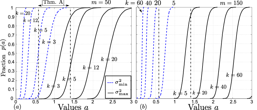
Figure 2: Means $p(a)=\mathbb{E}U_{n}(a)$ for predicting the concentration of $U_{n}(a)$. Shown for the Gaussian case, $(a)$ $m=50$ and $(b)$ $m=150$.

Table I reproduces a sample of (asymptotic) estimates for both $\sigma^{2}_{\scriptsize\mbox{max}}$ and $\sigma^{2}_{\scriptsize\mbox{min}}$ cases, taken from [21]. These estimates are derived for “worst-case” analysis, under assumption that every entry $A_{ij}$ of $\boldsymbol{A}$ is IID and Gaussian distributed (i.e., $A_{ij}$ is Gaussian with variance $1/m$). Table I presents the estimates according to fixed ratios $k/m$ and $m/n$. To compare, Figure 2 shows the expectations $p(a)=\mathbb{E}U_{n}(a)$. The values $p(a)$ are interpreted as fractions, and as $n/k$ becomes large $p(a)$ is approached by $U_{n}(a)$ within a stipulated error $\epsilon_{n}$. Figure 2 is empirically obtained, though note that in Gaussian case for $p(a)$ we also have exact expressions [32, 35], and the Bartlett decomposition [36], available. Again $p(a)$ is a marginal quantity (i.e. does not depend on $n$) and simulation is reasonably feasible. In the spirit of non-asymptotics, we consider relatively small $k,m$ values as compared to other works [21, 20]; these adopted values are nevertheless “practical”, in the sense they come an implementation paper [17].

TABLE I: Asymptotic Lower and Upper Bounds on “Worst-Case” Eigenvalues, [21]

		Minimum: $\sigma^{2}_{\mbox{\scriptsize min}}$			Maximum: $\sigma^{2}_{\mbox{\scriptsize max}}$
		$m/n$			$m/n$
		0.1	0.3	0.5	0.1	0.3	0.5
$k/m$	0.1	0.095	0.118	0.130	3.952	3.610	3.459
	0.2	0.015	0.026	0.034	5.587	4.892	4.535
	0.3	0.003	0.006	0.010	6.939	5.806	5.361

Differences are apparent from comparing “average-case” (Figure 2) and “worst-case” (Table I) behavior. Consider $k/m=0.3$ where Table I shows for all undersampling ratios $m/n$, the worst-case estimate of $\sigma^{2}_{\scriptsize\mbox{min}}$ is very small, approximately $0.01$. But for fixed $m=50$ and $m=150$, Figures 2$(a)$ and $(b)$ show that for respectively $k=0.3\cdot(150)=15$ and $k=45$, a large fraction of subsets $\mathcal{S}$ seem to have $\sigma^{2}_{\scriptsize\mbox{min}}(\boldsymbol{\Phi}_{\mathcal{S}})$ lying above $0.1$. From Table I, the estimates for $\sigma^{2}_{\scriptsize\mbox{min}}$ gets worse (i.e., gets smaller) as $m/n$ decreases. But the error $\epsilon_{n}(a)$ in Theorem 1 vanishes with larger $n/k$. For the other $\sigma^{2}_{\scriptsize\mbox{max}}$ case, we similarly observe that the values in Table I also appear more “pessimistic”.

We emphasize that Theorem 1 holds regardless of distribution. Figure 3 is the counterpart figure for Bernoulli and Uniform cases (i.e., each entry $A_{ij}$ is respectively drawn uniformly from $\{-1/\sqrt{m},1/\sqrt{m}\}$, or $\{a\in\mathbb{R}:|a|\leq\sqrt{3/m}\}$), shown for $m=50$. Minute differences are seen when comparing with previous Figure 2. For $k=3$, we observe the fraction $p(a)$ corresponding to $\sigma^{2}_{\scriptsize\mbox{max}}$ to be roughly 0.95 in the latter case, whereas in the former we have roughly $0.9$ in Figure 3$(a)$, and $0.88$ in Figure 3$(b)$.

Remark 1.

Exponential bounds on $\Pr\{\min_{\mathcal{S}}\sigma_{\scriptsize\mbox{min}}^{2}(\boldsymbol{A}_{\mathcal{S}})<1-\delta\}$ and $\Pr\{\max_{\mathcal{S}}\sigma_{\scriptsize\mbox{max}}^{2}(\boldsymbol{A}_{\mathcal{S}})>1+\delta\}$ for $\max(\delta,\sqrt{k/m})<\sqrt{2}-1$, see (3), employed in “worst-case” analyses, give the optimal $m=\mathcal{O}(k\log(n/k))$ rate, see [1, 37, 12]. However the implicit constants are inherently not too small (i.e., these constants cannot be improved).

These comparisons motivate “average-case” analysis. Marked out on Figures 2 and 3 are the ranges for which $\sigma^{2}_{\scriptsize\mbox{max}}$ and $\sigma^{2}_{\scriptsize\mbox{min}}$ must lie to apply Theorem A (“worst-case” analysis). In the cases shown above, the observations are somewhat disappointing - even for small $k$ values, a substantial fraction of eigenvalues lie outside of the required range. Thankfully, there exist “average-case” guarantees, e.g., previous Theorems B and C, addressed in the next section.

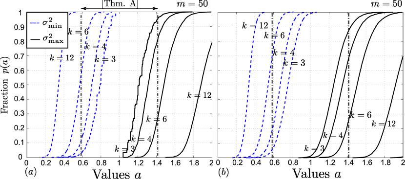
Figure 3: Means $p(a)=\mathbb{E}U_{n}(a)$ for $m=50$ and the $(a)$ Bernoulli and $(b)$ Uniform cases.

IV U-statistics & “Average-case” Recovery Guarantees

IV-A Counting argument using U-statistics

Previously we had explained how the invertability conditions required by Theorems B and C naturally relate to U-statistics. We now go on to discuss the other conditions, whereby the relationship may not be immediate. We begin with the projections conditions, in particular the worst-case projections condition. For given $\boldsymbol{\Phi}$, we need to upper bound the fraction of subsets $\mathcal{S}$, for which there exists at least one column $\boldsymbol{\phi}_{j}$ where $j\notin\mathcal{S}$, such that $||\boldsymbol{\Phi}_{\mathcal{S}}^{\dagger}\boldsymbol{\phi}_{j}||_{{\infty}}$ exceeds some value $a$. To this end, let $\mathcal{R}$ denote a size-$(k+1)$ subset, and ${\mathcal{R}\setminus\{j\}}$ is the size-$k$ subset excluding the index $j$. Consider the bounded kernel $g:\mathbb{R}^{m\times(k+1)}\times\mathbb{R}\mapsto\mathbb{R}_{[0,1]}$ set as

$$g(\bf A,a)=\frac{1}{k+1}\sum_{j=1}^{k+1}\mathbb{1}\left\{||\bf A_{{\mathcal{R}\setminus\{j\}}}^{\dagger}\bf a_{j}||_{{\infty}}>a\right\},$$ (12)

where here $\mathcal{R}=\{1,2,\cdots,k+1\}$, and $\bf a_{j}$ denotes the $j$-th column of $\bf A$. Consider the U-statistic with bounded kernel (12). We claim that

$$(n -k)\cdot U_{n}(a)$$

$$=\frac{n-k}{(k+1){n\choose k+1}}\sum_{\mathcal{R}}\!\sum_{j\in\mathcal{R}}\mathbb{1}\left\{||\boldsymbol{\Phi}_{\mathcal{R}\setminus\{j\}}^{\dagger}\boldsymbol{\phi}_{j}||_{{\infty}}>a\right\},$$

$$=\frac{1}{{n\choose k}}\sum_{\mathcal{S}}\!\sum_{j\notin\mathcal{S}}\mathbb{1}\left\{||\boldsymbol{\Phi}_{\mathcal{S}}^{\dagger}\boldsymbol{\phi}_{j}||_{{\infty}}>a\right\},$$

where the summations over $\mathcal{R}$ and $\mathcal{S}$ are over all size-$(k+1)$ subsets, and all size-$k$ subsets, respectively. The first equality follows from Definition 1 and (12). The second equality requires some manipulation. First the coefficient ${n\choose k}^{-1}$ follows from the binomial identity ${n\choose k+1}\cdot(k+1)={n\choose k}\cdot(n-k)$. Next for some subset $\mathcal{S}$ and index $j$, write the indicator $\mathbb{1}\left\{||\boldsymbol{\Phi}_{\mathcal{S}}^{\dagger}\boldsymbol{\phi}_{j}||_{{\infty}}>a\right\}$ as $\mathbb{1}_{\mathcal{S},j}$ for brevity’s sake. By similar counting that proves the previous binomial identity, we argue $\sum_{\mathcal{R}}\sum_{j\in\mathcal{R}}\mathbb{1}_{{\mathcal{R}\setminus\{j\}},j}=\sum_{\mathcal{S}}\sum_{j\notin\mathcal{S}}\mathbb{1}_{\mathcal{S},j}$, which then proves the claim. Imagine a grid of “pigeon-holes”, indexed by pairs $(\mathcal{S},j)$, where $j\notin\mathcal{S}$. For each size-$(k+1)$ subset $\mathcal{R}$, we assign $k+1$ indicators $\mathbb{1}_{{\mathcal{R}\setminus\{j\}},j}$ to $k+1$ pairs $(\mathcal{S},j)$. No “pigeon-hole” gets assigned more than once. In fact we infer from the binomial identity, that every “pigeon-hole” is in fact assigned exactly once, and argument is complete.

Similarly for the small projections condition, we define a different bounded kernel $g:\mathbb{R}^{m\times(k+1)}\times\mathbb{R}\mapsto\mathbb{R}_{[0,1]}$ as

$$g(\bf A,a)=\frac{1}{2^{k}(k+1)}\sum_{\ell=1}^{2^{k}}\sum_{j=1}^{k+1}\mathbb{1}\left\{\left|(\bf A_{{\mathcal{R}\setminus\{j\}}}^{\dagger}\bf a_{j})^{T}\boldsymbol{\beta}_{\ell}\right|>a\right\},$$ (13)

where $\mathcal{R}=\{1,2,\cdots,k+1\}$, and $\bf a_{j}$ denotes the $j$-th column of $\bf A$, and $\boldsymbol{\beta}_{1},\boldsymbol{\beta}_{2},\cdots,\boldsymbol{\beta}_{2^{k}}$ enumerate all $2^{k}$ unique sign-vectors in the set $\{-1,1\}^{k}$. By similar arguments as before, we can show for the U-statistic $U_{n}(a)$ of $\boldsymbol{\Phi}$ corresponding to the bounded kernel (13) satisfies

$$(n-k)\cdot U_{n}(a)\!\!\! = \!\!\!\frac{1}{2^{k}{n\choose k}}\sum_{\ell=1}^{2^{k}}\sum_{\mathcal{S}}\!\sum_{j\notin\mathcal{S}}\mathbb{1}\left\{\left|(\boldsymbol{\Phi}_{\mathcal{S}}^{\dagger}\boldsymbol{\phi}_{j})^{T}\boldsymbol{\beta}_{\ell}\right|>a\right\},$$

For indicators $\mathbb{1}_{\mathcal{S},j}$, note that $\sum_{j\notin\mathcal{S}}\mathbb{1}_{\mathcal{S},j}\geq 1$ if at least one indicator satisfying $\mathbb{1}_{\mathcal{S},j}=1$, and we proved the following.

Proposition 1.

Let $U_{n}(a_{3})$ be the U-statistic of $\boldsymbol{\Phi}$, corresponding to the bounded kernel $g(\bf A,a_{3})$ in (12). Then the fraction of subsets $\mathcal{S}$ of size-$k$, for which the worst-case projections condition is violated for some $a_{3}\in\mathbb{R}$, is at most $(n-k)\cdot U_{n}(a_{3})$. Similarly if $U_{n}(a_{2})$ corresponds to $g(\bf A,a_{2})$ in (13), the fraction sign-subset pairs $(\boldsymbol{\beta},\mathcal{S})$, for which the small projections condition is violated for some $a_{2}\in\mathbb{R}$, is at most $(n-k)\cdot U_{n}(a_{2})$.

Referring back to Theorem B, we point out that the small projections condition is more stringent than the worst-case projections condition. We mean the following: in the former case, the value $a_{2}$ must be chosen such that $a_{2}<1$; in the latter case, the value $a_{3}$ is allowed to be larger than $1$, its size only affects the constant $2a_{3}/(1-a_{2})$ appearing in the error estimate $||\boldsymbol{\alpha}_{\mathcal{S}}^{*}-\boldsymbol{\alpha}_{\mathcal{S}}||_{{1}}$. In fact if the signal $\boldsymbol{\alpha}$ is $k$-sparse, then $||\boldsymbol{\alpha}-\overline{\boldsymbol{\alpha}}_{k}||_{{1}}=0$ and the size of $a_{3}$ is inconsequential, i.e., the worst-case projections condition is not required in this special case. In this special case, it is best to set $a_{2}=1-\epsilon$ for some arbitrarily small $\epsilon$. Theorem B is in fact a stronger version of Fuchs’ early work on $\ell_{0}/\ell_{1}$-equivalence [5]. In the same respect, Donoho & Tanner also produced early seminal results from counting faces of random polytopes [23, 22].

Figure 4 shows empirical evidence, where the $k,m,n$ values are inspired by practical system sizes taken from an implementation paper [17]. These experiments consider $\boldsymbol{\Phi}$ sampled from Gaussian matrices $\boldsymbol{A}$, exactly $k$-sparse signals with non-zero $\alpha_{i}$ sampled from $\{-1,1\}$, and uses $\ell_{1}$-minimization recovery (1). Figure 4$(a)$ plots simulated (sparsity pattern recovery) results for 3 measurement sizes $m=50,100$ and $150$ and block sizes $n\geq 200$ and $n\leq 3000$. For example the contour marked “0.1”, delineates the $k,n$ values for which recovery fails for a 0.1 fraction of (random) sparsity patterns (sign-subset pairs $(\boldsymbol{\beta},\mathcal{S})$). We examine the U-statistic $U_{n}(a_{2})$ with kernel (13), related to the small projections condition. Since $\boldsymbol{A}$ has Gaussian distribution, we set $a_{2}=1$ in the kernel $g(\bf A,a_{2})$, as $\Pr\{(\boldsymbol{A}_{\mathcal{S}}^{\dagger}\boldsymbol{A}_{i})^{T}\boldsymbol{\beta}=1\}=0$ for any $(\boldsymbol{\beta},\mathcal{S})$ and $j\notin\mathcal{S}$. Figure 4$(b)$ plots the expectation $(n-k)\cdot p(1)$, where $p(1)=\mathbb{E}U_{n}(1)=\mathbb{E}g(\boldsymbol{A}_{\mathcal{R}},1)$ for any size-$(k+1)$ subset $\mathcal{R}$. Again the contour marked “0.1”, delineates the $k,n$ values for which $(n-k)\cdot p(1)=0.1$. Here the values $p(1)$ are empirical. We observe that both Figures 4$(a)$ and $(b)$ are remarkably close for fractions $0.5$ and smaller. Figures 4$(c)$ incorporates the large deviation error $\epsilon_{n}$ given in Theorem 1 (in doing so, we assume $n$ sufficiently large). The bound is still reasonably tight for fractions $\leq 0.5$. Comparing with recent Donoho & Tanners’ (also “average-case”) results for $\ell_{1}$-recovery (for only the noiseless case), taken from [23]. For fractions $0.5$ and $0.01$, we observe that for system parameters $m=50$ and $n\leq 1000$ (chosen in hardware implementation [17]), we do not obtain reasonable predictions. For $m=100$, the bounds [23] work only for very small block lengths $n\leq 300$. The only reasonable case here is $m=150$, where the bounds [23] perform better than ours only for lengths $n\leq 400$ (i.e., Figure 4$(c)$ shows that for $n=300$, the large deviation bounds predict a 0.01 fraction of size $k=5$ unrecoverable sparsity patterns, but [23] predict a 0.01 fraction of size $k=11$ unrecoverable sparsity patterns).

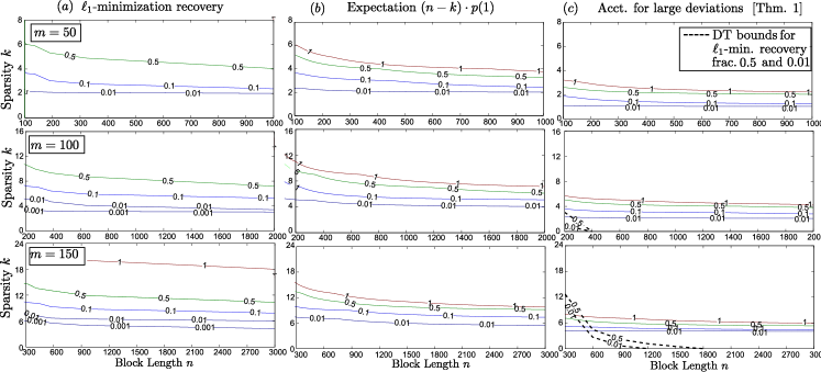
Figure 4: Gaussian case. Comparing $(a)$ empirical results for $\ell_{1}$-minimization recovery, $(b)$ mean parameter $(n-k)\cdot p(1)$ (empirically obtained), and $(c)$ after accounting for large deviations (Thm. 1). We show cases $m=50,100$ and $150$. We also compare with Donoho & Tanners’ (DT) large deviation bounds [23].

The above experiments suggest the deviation error $\epsilon_{n}(a)$ in Theorem 1 to be over-conservative. Fortunately in the next two subsections (pertaining to U-statistics treastise of $\ell_{1}$-recovery Theorem B (Section IV-B), and LASSO recovery Theorem C (Subsection IV-C)), this conservative-ness does not show up from a rate standpoint (it only shows up in implicit constants). In fact by empirically “adjusting” these constants, we find good measurement rate predictions (akin to moving from Figure 4$(c)$ to $(b)$).

IV-B Rate analysis for $\ell_{1}$-recovery (Theorem B)

In “worst-case” analysis, it is well-known that it is sufficient to have measurements $m$ on the order of $k\log(n/k)$, in order to have the restricted isometry constants $\delta_{k}$ defined by (2), satisfy the conditions in Theorem A. We now go on to show that for “average-case”, a similar expression for this rate can be obtained. To this end we require tail bounds on salient quantities. Such bounds have been obtained for the small projections condition, see [6, 7, 25], where typically an equiprobable distribution is assumed over the sign-vectors $\boldsymbol{\beta}_{\ell}$. To our knowledge these techniques were born from considering deterministic matrices. Since $\boldsymbol{\Phi}$ is randomly sampled here, we proceed slightly differently (though essentially using similar ideas) without requiring this random signal model. For simplicity, the bound assumes zero mean matrix entries, either i) Gaussian or ii) bounded.

Proposition 2.

Let $\boldsymbol{A}$ be an $m\times n$ random matrix, whereby its columns $\boldsymbol{A}_{i}$ are identically distributed. Assume every entry $A_{ij}$ of $\boldsymbol{A}$ has zero mean, i.e., $\mathbb{E}A_{ij}=0$. Let every $A_{ij}$ be either i) Gaussian with variance $1/m$, or ii) bounded RVs satisfying $|A_{ij}|\leq 1/\sqrt{m}$. Let the rows $[A_{i1},A_{i2},\cdots,A_{in}]$ of $\boldsymbol{A}$ be IID.

Let $\mathcal{S}$ be a size-$k$ subset, and let index $\omega$ be outside of $\mathcal{S}$, i.e., $\omega\notin\mathcal{S}$. Then for any sign vector $\boldsymbol{\beta}$ in $\{-1,1\}^{k}$, we have

$$\Pr\left\{\left|(\boldsymbol{A}_{\mathcal{S}}^{\dagger}\boldsymbol{A}_{\omega})^{T}\boldsymbol{\beta}\right|>a\right\}\leq ~{}2\exp\left(-\frac{ma^{2}\delta}{2k}\right)$$

$$+\Pr\{\sigma^{2}_{\scriptsize\mbox{min}}(\boldsymbol{A}_{\mathcal{S}})\leq\delta\}$$ (14)

for any positive $\delta\in\mathbb{R}$.

Proof.

For $\tau\in\mathbb{R}$, let $\mathcal{E}(\tau)=\{\boldsymbol{\beta}^{T}(\boldsymbol{A}_{\mathcal{S}}^{T}\boldsymbol{A}_{\mathcal{S}})^{\dagger}\boldsymbol{\beta}\leq\tau\}$ where $\mathcal{E}(\tau)$ is an probabilistic event. Let $\mathcal{E}_{c}(\tau)$ denote the complementary event. Bound the probability as

$$\Pr\left\{\left|(\boldsymbol{A}_{\mathcal{S}}^{\dagger}\boldsymbol{A}_{\omega})^{T}\boldsymbol{\beta}\right|>a\right\}\leq \Pr\left\{\left.\left|(\boldsymbol{A}_{\mathcal{S}}^{\dagger}\boldsymbol{A}_{\omega})^{T}\boldsymbol{\beta}\right|>a\right|\mathcal{E}(\tau)\right\}$$

$$+\Pr\{\mathcal{E}_{c}(\tau)\}.$$ (15)

We upper bound the first term as follows. Denote constants $c_{1},c_{2},\cdots,c_{m}$. For entries $(\boldsymbol{A}_{\omega})_{i}$ of $\boldsymbol{A}_{\omega}$, consider the sum $\sum_{i=1}^{m}c_{i}\cdot(m^{-\frac{1}{2}}\boldsymbol{A}_{\omega})_{i}=\frac{1}{m}\sum_{i=1}^{m}c_{i}X_{i}$, where RVs $X_{i}$ satisfy $X_{i}=(\sqrt{m}\boldsymbol{A}_{\omega})_{i}$. By standard arguments (see Supplementary Material -B) we have the double-sided bound $\Pr\left\{\left|\sum_{i=1}^{m}c_{i}X_{i}\right|>mt\right\}\leq 2\exp\left(-(mt)^{2}/(2\cdot||\bf c||_{{2}}^{2})\right)$, where vector $\bf c$ equals $[c_{1},c_{2},\cdots,c_{m}]^{T}$.

Next write $(\boldsymbol{A}_{\mathcal{S}}^{\dagger}\boldsymbol{A}_{\omega})^{T}\boldsymbol{\beta}=(\sqrt{m}\cdot\boldsymbol{\beta}^{T}\boldsymbol{A}_{\mathcal{S}}^{\dagger})(m^{-\frac{1}{2}}\boldsymbol{A}_{\omega})$. When conditioning on $\boldsymbol{\beta}^{T}\boldsymbol{A}_{\mathcal{S}}^{\dagger}$, then $\sqrt{m}\cdot\boldsymbol{\beta}^{T}\boldsymbol{A}_{\mathcal{S}}^{\dagger}$ is fixed, say equals some vector $\bf c$. Put $X_{i}=(\sqrt{m}\boldsymbol{A}_{\omega})_{i}$ and $X_{i}$’s are independent (by assumed independence of the rows of $\boldsymbol{A}$). Then use the above bound for $\Pr\left\{\sum_{i=1}^{m}c_{i}X_{i}>t\right\}$, set $t=a$ and conclude

$$\Pr\left\{\left.\left|(\boldsymbol{A}_{\mathcal{S}}^{\dagger}\boldsymbol{A}_{\omega})^{T}\boldsymbol{\beta}\right|>a\right|\boldsymbol{\beta}^{T}\boldsymbol{A}_{\mathcal{S}}^{\dagger}\right\}$$

$$\leq 2\exp\left(-\frac{(ma)^{2}}{2m||\boldsymbol{\beta}^{T}\boldsymbol{A}_{\mathcal{S}}^{\dagger}||_{{2}}^{2}}\right)=2\exp\left(-\frac{ma^{2}}{2\cdot\boldsymbol{\beta}^{T}(\boldsymbol{A}_{\mathcal{S}}^{T}\boldsymbol{A}_{\mathcal{S}})^{\dagger}\boldsymbol{\beta}}\right),$$ (16)

where the last equality follows from the identity $\boldsymbol{A}_{\mathcal{S}}^{\dagger}(\boldsymbol{A}_{\mathcal{S}}^{\dagger})^{T}=(\boldsymbol{A}_{\mathcal{S}}^{T}\boldsymbol{A}_{\mathcal{S}})^{\dagger}$. Further conclude that the first term in (15) is bounded by $2\exp(-ma^{2}/(2\tau))$, due to further conditioning on the event $\mathcal{E}(\tau)=\{\boldsymbol{\beta}^{T}(\boldsymbol{A}_{\mathcal{S}}^{T}\boldsymbol{A}_{\mathcal{S}})^{\dagger}\boldsymbol{\beta}\leq\tau\}$.

To bound the second term, let $\varsigma_{\scriptsize\mbox{max}}(\bf A)$ denote the maximum eigenvalue of matrix $\bf A$. Since $\boldsymbol{A}_{\mathcal{S}}^{T}\boldsymbol{A}_{\mathcal{S}}$ is positive semidefinite, note that $\boldsymbol{\beta}^{T}(\boldsymbol{A}_{\mathcal{S}}^{T}\boldsymbol{A}_{\mathcal{S}})^{\dagger}\boldsymbol{\beta}$ is upper bounded by $||\boldsymbol{\beta}||_{{2}}^{2}\cdot\varsigma_{\scriptsize\mbox{max}}((\boldsymbol{A}_{\mathcal{S}}^{T}\boldsymbol{A}_{\mathcal{S}})^{\dagger})$, which equals $k\cdot\varsigma_{\scriptsize\mbox{max}}((\boldsymbol{A}_{\mathcal{S}}^{T}\boldsymbol{A}_{\mathcal{S}})^{\dagger})$. Furthermore $\varsigma_{\scriptsize\mbox{max}}((\boldsymbol{A}_{\mathcal{S}}^{T}\boldsymbol{A}_{\mathcal{S}})^{\dagger})\leq 1/\sigma^{2}_{\scriptsize\mbox{min}}(\boldsymbol{A}_{\mathcal{S}})$, where here $\sigma_{\scriptsize\mbox{min}}(\bf A)$ is the minimum singular value of $\bf A$. Thus $\Pr\{\mathcal{E}_{c}(\tau)\}\leq\Pr\{k/\sigma^{2}_{\scriptsize\mbox{min}}(\boldsymbol{A}_{\mathcal{S}})>\tau\}$. Finally put $\tau=\delta k$ to get $\Pr\{\mathcal{E}_{c}(\tau)\}\leq\Pr\{\sigma^{2}_{\scriptsize\mbox{min}}(\boldsymbol{A}_{\mathcal{S}})\leq\delta^{-1}\}$. ∎

Proposition 2 is used as follows. First recall that previous Proposition 1 allows us to upper bound the fraction $u_{2}$ of sign-subset pairs $(\boldsymbol{\beta},\mathcal{S})$ failing the small projections condition, with the (scaled) U-statistic $(n-k)\cdot U_{n}(a_{2})$ with kernel $g$ in (13) and $|\mathcal{S}|=k$. By Theorem 1 the quantity $(n-k)\cdot U_{n}(a_{2})$ concentrates around $(n-k)\cdot p(a_{2})$, where $p(a_{2})=\mathbb{E}g(\boldsymbol{A}_{\mathcal{R}},a_{2})$, where $g$ in (13) is defined for size-$(k+1)$ subsets $\mathcal{R}$. We use Proposition 2 to upper estimate $p(a_{2})$ using the RHS of (14). Indeed verify that $p(a_{2})=2^{-k}\sum_{\ell}\Pr\{|(\boldsymbol{A}_{\mathcal{S}}^{\dagger}\boldsymbol{A}_{\omega})^{T}\boldsymbol{\beta}_{\ell}|>a_{2}\}$ for any $S$ and $\omega\notin S$, and the bound (14) holds for any $\boldsymbol{\beta}=\boldsymbol{\beta}_{\ell}$. Now $p(a_{2})$ is bounded by two terms. By $u_{2}\leq(n-k)\cdot U_{n}(a_{2})$, thus to have $u_{2}$ small, we should have the (scaled) first term $2(n-k)\cdot\exp(-ma_{2}^{2}\delta/(2k))$ of (14) to be at most some small fraction $u$. This requires

$$m\geq\operatorname{const}\cdot k\log\left(\frac{n-k}{u}\right)$$ (17)

with $\operatorname{const}=2/(a_{2}^{2}\delta)$ (and we dropped an insignificant $\log 2$ term). Next, for $m\geq 2k$ and $\delta<(0.29)^{2}$, we can bound the second term $\Pr\{\sigma^{2}_{\scriptsize\mbox{min}}(\boldsymbol{A}_{\mathcal{S}})\leq\delta\}$ of (14) by $\exp(-m\cdot(0.29-\sqrt{\delta})^{2}/c_{1})$ where $c_{1}$ is some constant, see [27], Theorem 5.39. Roughly speaking, $\sigma^{2}_{\scriptsize\mbox{min}}(\boldsymbol{A}_{\mathcal{S}})\geq 0.29$ with “high probability”. Figures 2 and 3 (in the previous Section III) empirically support this fact. Again to have $u_{2}$ small the second term of (14) must be small. This requires $(n-k)\cdot\exp(-m\cdot(0.29-\sqrt{\delta})^{2}/c_{1})\leq u$ for some small fraction $u$, in which it suffices to have $m$ satisfy (17) with $\operatorname{const}=c_{1}/(0.29-\sqrt{\delta})^{2}$.

For the invertability condition in Theorem B, we also need to upper bound the corresponding fraction $u_{1}$ of size-$k$ subsets $\mathcal{S}$. We simply use an U-statistic $U_{n}(a_{1})$ with kernel $g(\bf A,a_{1})=\mathbb{1}\left\{\sigma_{\scriptsize\mbox{min}}(\bf A)>a_{1}\right\}$ for some positive $a_{1}$ (see also Theorem C). Here Proposition 1 is not needed. To make $p(a_{1})$ small, where $p(a_{1})=\mathbb{E}g(\boldsymbol{A}_{\mathcal{S}},a_{1})$, use the previous bound $p(a_{1})\leq\exp(-m\cdot(0.29-a_{1})^{2}/c_{1})$, where we set $a_{1}=\sqrt{\delta}$ with $a_{1}\leq 0.29$. Clearly $p(a_{1})$ cannot exceed some fraction $u$, if $m$ satisfies (17) with $\operatorname{const}=c_{1}/(0.29-a_{1})^{2}$.

For the time being consider exactly $k$-sparse signals $\boldsymbol{\alpha}$. In this special case the worst-case projections condition in Theorem B is superfluous (i.e., with no consequence $a_{3}$ can be arbitrarily big) - only invertability and small projections conditions are needed. While we have yet to consider the large deviation error $\epsilon_{n}(a)$ from Theorem 1, doing so will not drastically change the rate. For $U_{n}(a)$ with kernel $g$ and $p(a)$, where $p(a)=\mathbb{E}g(\boldsymbol{A},a)$, almost surely

$$\!\!\!\!\!\!\!\!\!U_{n}(a)\leq p(a)+\epsilon_{n}(a)\!\!\! \leq \!\!\!(p(a))^{\frac{1}{2}}+\sqrt{2p(a)\omega^{-1}\log\omega}$$ (18)

$$\leq \!\!\!(p(a))^{\frac{1}{2}}\left(1+\sqrt{2\omega^{-1}\log\omega}\right)$$

where the second inequality follows because $p(a)\leq 1$, and by setting $\omega=n/k$. Taking $\log$ of the RHS, we obtain $(1/2)\log p(a)+\log(1+\sqrt{2\omega^{-1}\log\omega})$. Note $\log(1+\sqrt{2\omega^{-1}\log\omega})\leq\sqrt{2\omega^{-1}\log\omega}$, since $\log(1+\alpha)\leq\alpha$ holds for all positive $\alpha$. For the small projections condition, bound $(p(a))^{\frac{1}{2}}$ by the sum of the square-roots of each term in (14). Then to have $u_{2}\leq(n-k)\cdot U_{n}(a_{2})\leq 2u$, it follows similarly as before that it suffices that (see Supplementary Material -C)

$$m\geq\operatorname{const}\cdot k\left[\log\left(\frac{n-k}{u}\right)+\sqrt{2\cdot(k/n)\log(n/k)}\right]$$ (19)

with $\operatorname{const}=\max(4/(a_{2}^{2}\delta),2c_{1}/(0.29-\sqrt{\delta})^{2})$ where we had set $\sqrt{\delta}=a_{1}$ (we dropped an insignificant $\log 2$ term). For invertability condition do the same. To have $u_{1}=U_{n}(a_{1})\leq u$ it suffices that $m$ satisfies (19) with the same $\operatorname{const}$. Observe that the term $\sqrt{2\cdot(k/n)\log(n/k)}$ is at most 1, and vanishes with high undersampling (small $k/n$). Hence (17) and (19) are similar from a rate standpoint.

We conclude the following: for exactly $k$-sparse signals the rate (19) suffices to recover at least $1-3u$ fraction of sign-subset $(\boldsymbol{\beta},\mathcal{S})$ pairs. While $\operatorname{const}$ in (19) must be at least $4$ (recall that Figure 4$(c)$ was somewhat pessimistic), for matrices with Gaussian entries we empirically find that $\operatorname{const}$ is inherently smaller, whereby $\operatorname{const}\approx 1.8$. This is illustrated in Figure 5, for two fractions $0.1$ and $0.01$ of unrecoverable sign-subset pairs. We observe good match with simulation results shown in the previous Figure 4$(a)$, and quantities $(n-k)\cdot p(1)$ plotted in Figure 4$(b)$. For example, $m=150$ suffices for a 0.01 fractional recovery failure, for $n=300\sim 1000$ and $k=6\sim 7$, and for 0.1 fraction then $k=7\sim 10$. We conjecture possible improvment for $\operatorname{const}$.

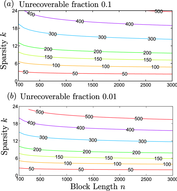
Figure 5: Measurement rates predicted by equation (19), with $\operatorname{const}$ taken to equal $1.8$, required to recover at least $1-3u=0.9$ and $0.99$ fractions of sign-subset pairs $(\boldsymbol{\beta},\mathcal{S})$ (when the signal is exactly $k$-sparse), shown respectively in $(a)$ and $(b)$.

In the more general setting for approximately $k$-sparse signals, we can also have rate (19). To see this, observe that Proposition 2 also delivers an exponential bound for the worst-case projections condition, see (12). This is because $||\boldsymbol{A}_{\mathcal{S}}^{\dagger}\boldsymbol{A}_{\omega}||_{{1}}=\max_{\ell:\;1\leq\ell\leq 2^{k}}|(\boldsymbol{A}_{\mathcal{S}}^{\dagger}\boldsymbol{A}_{\omega})^{T}\boldsymbol{\beta}_{\ell}|$, and we take a union bound over $2^{k}$ terms. Set $a_{3}=a_{2}\sqrt{k}$, where $a_{2}$ and $a_{3}$ respectively correspond to small projections and invertability conditions. Then we proceed similarly as before (see Supplementary Material -C) to show that the rate for recovering at least $1-5u$ fraction of $(\boldsymbol{\beta},\mathcal{S})$ pairs suffices to be (19). The following is the main result summarizing the exposition so far.

Theorem 2.

Let $\boldsymbol{\Phi}$ be an $m\times n$ matrix, where assume $n$ sufficiently large for Theorem 1 to hold. Sample $\boldsymbol{\Phi}=\boldsymbol{A}$ whereby the entries $A_{ij}$ are IID, and are Gaussian or bounded (as stated in Proposition 2). Then all three conditions in $\ell_{1}$-recovery guarantee Theorem B for $(\boldsymbol{\beta},\mathcal{S})$ with $|\mathcal{S}|=k$, with the invertability condition taken as $\sigma_{\scriptsize\mbox{min}}(\boldsymbol{\Phi}_{\mathcal{S}})\geq a_{1}$ with $a_{1}\leq 0.29$. and with $a_{3}=a_{1}\sqrt{k}$, are satisfied for $u_{1}+u_{2}+u_{3}=5u$ for some small fraction $u$, if $m$ is on the order of (19) with $\operatorname{const}=\max(4/(a_{1}a_{2})^{2},2c_{1}/(0.29-a_{1})^{2})$, and $c_{1}$ depends on the distribution of $A_{ij}$’s. Note $\operatorname{const}\geq 4$.

In the exactly $k$-sparse case where only the first 2 conditions are required, this improves to $u_{1}+u_{2}=3u$.

We end this subsection with two comments on the rate (19) derived here for “average-case” analysis. Firstly (19) is very similar to that of $k\log(n/k)$ for “worst-case” analysis. This justifies the counting employed in previous Subsection IV-A, Proposition 1, and is reassuring since we know that “worst-case” analysis provides the optimal rate [1, 11]. Secondly to have (19) hold for the approximately $k$-sparse case, we lose a factor of $\sqrt{k}$ in the error estimate $||\boldsymbol{\alpha}^{*}_{\mathcal{S}}-\boldsymbol{\alpha}_{\mathcal{S}}||_{{1}}$, as compared to “worst-case” Theorem A. This is because we need to set $a_{3}=a_{2}\sqrt{k}$, as mentioned in the previous paragraph. However, the “average-case” analysis here achieves our primary goal, that is to predict well for system sizes $k,m,n$ when “worst-case” analysis becomes too pessimistic.

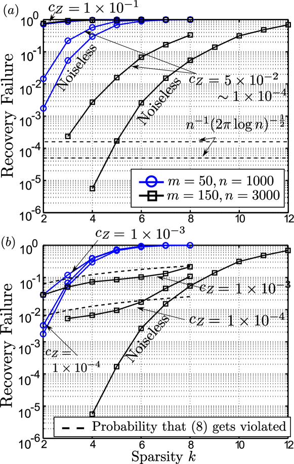
Figure 6: Empirical LASSO recovery performance, Bernoullli case. In $(a)$ the non-zero signal magnitudes $|\alpha_{i}|$ equal 1, and in $(b)$ they are in $\mathbb{R}_{[0,1]}$. Noise variances denoted $c_{Z}^{2}$.

IV-C Rate analysis for LASSO (Theorem C)

Next we move on to the LASSO estimate of [6]. Recall from (6) that the regularizer depends on the noise standard deviation $c_{Z}$, and the term $\theta_{n}=(1+a)\sqrt{2\log n}$ that depends on block length $n$ and some non-negative constant $a$ that we set. This constant $a$ impacts performance [6]. For matrices with Bernoulli entries, Figure 6 shows recovery failure rates for two data sets $m=50,n=1000$ and $m=150,n=1000$; the sparsity patterns (sign-subset pairs $(\boldsymbol{\beta},\mathcal{S})$) were chosen at random, and failure rates are shown for various sparsity values $k$, and noises $c_{Z}$. In Figure 6$(a)$ we set $a=0$, and in $(b)$ we set $a=1$. Also, in $(a)$ the non-zero signal magnitudes $|\alpha_{i}|$ are in $\{1,-1\}$, and in $(b)$ they are in $\mathbb{R}_{[0,1]}$. The performances are clearly different. “Threshold-like” behavior is seen in $(a)$ for both data sets, whereby the performances stay the same for $c_{Z}$ in the range $5\times 10^{-2}\sim 1\times 10^{-4}$, and then catastrophically failing for $c_{Z}=1\times 10^{-1}$. However in $(b)$, for various $c_{Z}$ the performances seem to be limited by a “noise-floor”. We see that in the noiseless limit (more specifically when $c_{Z}\rightarrow 0$), the performances become the same. In this subsection, we apply U-statistics on the various conditions of Theorem C, in particular the invertability and small projections conditions have already been discussed in the previous subsection. We account for the observations in Figure 6.

In the noiseless limit, the previously derived rate (19) holds. Here, the regularizer in (6) becomes so small that $a$ (equivalently $\theta_{n}$) does not matter. As mentioned in [5], LASSO then becomes equivalent to $\ell_{1}$-minimization (1), hence the (noiseless) performances in Figures 6$(a)$ and $(b)$ are the same. That is, in this special case the rate (19) suffices to recover at least $1-3u$ fraction of $(\boldsymbol{\beta},\mathcal{S})$. To test, take $k=4$, $n=3000$, and fraction $1-3u=1-6\times 10^{-6}$, and with $\operatorname{const}=1.8$ gives $153$, close to $m$ here which is set to $150$.

In the noisy case, we are additionally concerned with the noise conditions i) and ii), conditions (7) and (8), and invertability projections. Recall that the noise conditions are satisfied with probability $1-n^{-1}(2\pi\log n)^{-\frac{1}{2}}$, that goes to 1 superlinearly [6] (Proposition 4, Supplementary Material -A). The remaining conditions are influenced by the value $a$ set in the $\theta_{n}$ regularization term in (6).

In condition (7), the value $a$ sets the maximal value for $a_{2}$ (when $a=0$ then $a_{2}<0.2929$, and when $a=1$ then $a_{2}<0.6464$). This affects the small projections condition, to which constant $a_{2}$ belongs, which in turn affects performance. However from a rate standpoint (19) still holds, only now the value of $\operatorname{const}$ (which has the term $4/(a_{2}^{2}\delta)$) becomes larger.

In condition (8), the value $a$ affects the size of the term $a_{1}^{-1}+2a_{3}(1+a)$. The larger $a$ is, the more often (8) fails to satisfy. Here there are two constants $a_{1}$ and $a_{3}$. Recall $a_{1}$ belongs to the invertability condition discussed in the previous subsection, which holds with rate (19) with $\operatorname{const}=2c_{1}/(0.29-a_{1})^{2}$ and $a_{1}\leq 0.29$. Consider the case where the non-zero signal magnitudes $|\alpha_{i}|$ are independently drawn from $\mathbb{R}_{[0,1]}$. Then we observe $(\min_{i\in\mathcal{S}}|\alpha_{i}|)<t$ with probability $1-(1-t)^{k}$ where $t\in\mathbb{R}_{[0,1]}$ and $|\mathcal{S}|=k$. For $t$ set equal to the RHS of (8), this gives the probability that condition (8) fails. Figure 6$(b)$ shows good empirical match when setting $a_{1}=0.29$ and $a_{3}=1$, where the dotted curves predict the “error-floors” for various $k$, measurements $m=50$ and $m=150$, and noise $c_{Z}$. In the other case where $|\alpha_{i}|=1$ (as in Figure 6$(a)$), condition (8) remains un-violated as long as $c_{Z}$ (and $a_{1},a_{3},n$) allow the RHS to be smaller than 1. Figure 6$(a)$ suggests that for the appropriate choices for $a_{1},a_{3}$, condition (8) is always un-violated when $c_{Z}\leq 5\times 10^{-2}$, and violated when $c_{Z}\geq 1\times 1^{-1}$. For more discussion on noise effects see Supplementary Material -D.

The constant $a_{3}$ belongs to the remaining invertability projections condition. The fraction $u_{3}$ of size-$k$ subsets failing the invertability projections condition for some $a_{3}$, can be addressed using U-statistics. Consider the bounded kernel $g:\mathbb{R}^{m\times k}\times\mathbb{R}\rightarrow\mathbb{R}_{[0,1]}$, set as

$$g(\bf A,a)=\frac{1}{2^{k}}\sum_{\ell=1}^{2^{k}}\mathbb{1}\left\{(\bf A^{T}\bf A)^{\dagger}\boldsymbol{\beta}_{\ell}>a\right\}$$ (20)

where $\boldsymbol{\beta}_{\ell}\in\{-1,1\}^{k}$ and $(\bf A^{T}\bf A)^{\dagger}$ is the pseudoinverse of $\bf A^{T}\bf A$. Then $u_{3}=U_{n}(a_{3})$, and as before Theorem 1 guarantees the upper bound (18), which depends on $p(a_{3})$ where $p(a_{3})=\mathbb{E}g(\boldsymbol{A}_{\mathcal{S}},a_{3})$.

We go on to discuss a bound on $p(a_{3})$ under some general conditions. In [6], analysis on $p(a_{3})$ (see Lemma 3.5) requires $\sigma^{2}_{\scriptsize\mbox{max}}(\boldsymbol{A}_{\mathcal{S}})\leq 1.5$, a condition not explicitly required in Theorem C. Also, empirical evidence suggests not to assume that $\sigma^{2}_{\scriptsize\mbox{max}}(\boldsymbol{A}_{\mathcal{S}})\leq 1.5$. For $m=150$ and $k=5$ we see from Figure 6 that (in the noiseless limit) the failure rate is on the order of $1\times 10^{-4}$, but in Figure 2$(b)$ we see $\sigma^{2}_{\scriptsize\mbox{max}}(\boldsymbol{A}_{\mathcal{S}})>1.5$ occurs with much larger fraction 0.1. Hence we take a different approach. Using ideas behind Bauer’s generalization of Wielandt’s inequality [38], the following proposition allows $\sigma^{2}_{\scriptsize\mbox{max}}(\boldsymbol{A}_{\mathcal{S}})$ to arbitrarily exceed 1.5. Also, it does not assume any particular distribution on entries of $\boldsymbol{A}$.

Proposition 3.

Let $\mathcal{S}$ be a size-$k$ subset. Assume $k\geq 2$. Let $\boldsymbol{A}_{\mathcal{S}}$ be an $k\times n$ random matrix. Let $\delta_{\scriptsize\mbox{min}},\delta_{\scriptsize\mbox{max}}$ be some positive constants. For any sign vector $\boldsymbol{\beta}$ in $\{-1,1\}^{k}$, we have

$$\Pr\left\{||(\boldsymbol{A}_{\mathcal{S}}^{T}\boldsymbol{A}_{\mathcal{S}})^{\dagger}\boldsymbol{\beta}||_{{\infty}}>\frac{(\sqrt{k}+1)\cdot|\tau_{k}-1|}{\delta_{\scriptsize\mbox{min}}^{2}\cdot(\tau_{k}+1)}\cdot\right\}$$

$$~{}~{}~{}~{}~{}~{}~{}\leq~{}\Pr\{\mathcal{E}_{c}(\delta_{\scriptsize\mbox{min}},\delta_{\scriptsize\mbox{max}})\}$$ (21)

where $\mathcal{E}(\delta_{\scriptsize\mbox{min}},\delta_{\scriptsize\mbox{max}})=\{\delta_{\scriptsize\mbox{min}}\leq\sigma_{\scriptsize\mbox{min}}(\boldsymbol{A}_{\mathcal{S}})\leq\sigma_{\scriptsize\mbox{max}}(\boldsymbol{A}_{\mathcal{S}})\leq\delta_{\scriptsize\mbox{max}}\}$, and $\mathcal{E}_{c}(\delta_{\scriptsize\mbox{min}},\delta_{\scriptsize\mbox{max}})$ is the complementary event of $\mathcal{E}(\delta_{\scriptsize\mbox{min}},\delta_{\scriptsize\mbox{max}})$, and the constant $\tau_{k}$ satisfies

$$\tau_{k}=\tau_{k}(\delta_{\scriptsize\mbox{max}},\delta_{\scriptsize\mbox{min}})=\left(\frac{\delta_{\scriptsize\mbox{max}}}{\delta_{\scriptsize\mbox{min}}}\right)^{2}\cdot\frac{1+k^{-\frac{1}{2}}}{1-k^{-\frac{1}{2}}}.$$ (22)

We defer the proof for now. If $\boldsymbol{A}_{\mathcal{S}}^{T}\boldsymbol{A}_{\mathcal{S}}$ is “almost” an identity matrix, then we expect $||(\boldsymbol{A}_{\mathcal{S}}^{T}\boldsymbol{A}_{\mathcal{S}})^{-1}\boldsymbol{\beta}||_{{\infty}}\approx 1$ for any sign vector $\boldsymbol{\beta}$ (hence our above hueristic whereby we set $a_{3}=1$). Proposition 3 makes a slightly weaker (but relatively general) statement. Now for some appropriately fixed $\delta_{\scriptsize\mbox{max}}$ and $\delta_{\scriptsize\mbox{min}}$, we expect $\Pr\{\mathcal{E}_{c}(\delta_{\scriptsize\mbox{min}},\delta_{\scriptsize\mbox{max}})\}$ in (21) to drop exponentially in $m$. Just as the term $\Pr\{\sigma_{\scriptsize\mbox{min}}(\boldsymbol{A}_{\mathcal{S}})\leq\delta_{\scriptsize\mbox{min}}\}$ in Proposition 2 can be bounded by $\exp(-m\cdot(0.29-\delta_{\scriptsize\mbox{min}})^{2}/c_{1})$, we can bound $\Pr\{\sigma_{\scriptsize\mbox{max}}(\boldsymbol{A})>\delta_{\scriptsize\mbox{max}}\}\leq\exp(-m(\delta_{\scriptsize\mbox{max}}-1.71)^{2}/c_{1})$ for some $\delta_{\scriptsize\mbox{max}}\geq 1.71$. Roughly speaking, $\sigma_{\scriptsize\mbox{max}}(\boldsymbol{A}_{\mathcal{S}})\leq 1.71$ (or $\sigma^{2}_{\scriptsize\mbox{max}}(\boldsymbol{A}_{\mathcal{S}})\leq 2.92$) with “high probability”. We fix $\delta_{\scriptsize\mbox{min}}=a_{1}$, where $a_{1}$ belongs to the invertability condition.

So to bound $p(a_{3})$, both (20) and Proposition 3 imply $p(a_{3})\leq\Pr\{\mathcal{E}_{c}(\delta_{\scriptsize\mbox{min}},\delta_{\scriptsize\mbox{max}})\}$ for $a_{3}=(\sqrt{k}+1)\cdot|\tau_{k}-1|/(\delta_{\scriptsize\mbox{min}}^{2}\cdot(\tau_{k}+1))$. Now $\Pr\{\mathcal{E}_{c}(\delta_{\scriptsize\mbox{min}},\delta_{\scriptsize\mbox{max}})\}\leq 2\exp(-m\cdot t^{2}/c_{1})$, where we set $t=\delta_{\scriptsize\mbox{max}}-1.71=0.29-a_{1}$ and $\delta_{\scriptsize\mbox{min}}=a_{1}$. By (18), the rate (19) suffices to ensure $u_{3}=U_{n}(a_{3})\leq u$ for some fraction $u$, with the same $\operatorname{const}$. Thus we proved the other main theorem, similar to Theorem 2.

Theorem 3.

Let $\boldsymbol{\Phi}$ be an $m\times n$ matrix, , where assume $n$ sufficiently large for Theorem 1 to hold. Sample $\boldsymbol{\Phi}=\boldsymbol{A}$ whereby the entries $A_{ij}$ are IID, and are Gaussian or bounded (as stated in Proposition 2). Then all three invertability, small projections, and invertability projections conditions in LASSO Theorem C for $(\boldsymbol{\beta},\mathcal{S})$ with $|\mathcal{S}|=k\geq 2$, with $a_{1}\leq 0.29$, with $a_{2}$ satisfying (7) for some $a$ set in the regularizer $\theta_{n}$, and with $a_{3}=(\sqrt{k}+1)\cdot|\tau_{k}-1|/(a_{1}^{2}\cdot(\tau_{k}+1))$ for $\tau_{k}=\tau_{k}(1.42-a_{1},a_{1})$ in (22), are satisfied for $u_{1}+u_{2}+u_{3}=4u$ for some small fraction $u$, if $m$ is on the order of (19) with $\operatorname{const}=\max(4/(a_{1}a_{2})^{2},2c_{1}/(0.29-a_{1})^{2})$, and $c_{1}$ depends on the distribution of $A_{ij}$’s. Note $\operatorname{const}\geq 4$.

In the noiseless limit where only the first 2 conditions are required, this improves to $u_{1}+u_{2}=3u$.

Remark 2.

We emphasize again that the rate (19) is measured w.r.t. to the three conditions in Theorem 3. The probability for which both noise conditions i) and ii) are satisfied, and for which condition (8) imposed on $\min_{i\in\mathcal{S}}|\alpha_{i}|$ is satisfied, require additional consideration. For the former the probability is at least $1-n^{-1}(2\pi\log n)^{-\frac{1}{2}}$, see [6]. For the latter, it has to be derived based on signal statistics, e.g., for $|\alpha_{i}|\in\mathbb{R}_{[0,1]}$ then $(\min_{i\in\mathcal{S}}|\alpha_{i}|)>t$ is observed with probability $(1-t)^{k}$ with $|\mathcal{S}|=k$.

Note that the choice for $a_{3}$ in Theorem 3 implies $||(\boldsymbol{A}_{\mathcal{S}}^{T}\boldsymbol{A}_{\mathcal{S}})^{\dagger}\boldsymbol{\beta}||_{{\infty}}$ is roughly on the order $\sqrt{k}$. Indeed this is true since $\tau_{k}\geq 1$, and we note $\tau_{k}=(\delta_{\scriptsize\mbox{max}}/\delta_{\scriptsize\mbox{min}})^{2}+2k^{-\frac{1}{2}}+o(k^{-\frac{1}{2}})$, thus $\tau_{k}\approx(\delta_{\scriptsize\mbox{max}}/\delta_{\scriptsize\mbox{min}})^{2}$ for moderate $k$. Now LASSO recovery also depends on the probability that condition (8) holds. Our choice for $a_{3}$ causes the RHS of (8) to be roughly of the order $c_{Z}\sqrt{2k\log n}$. Compare this to [6] (see Theorem 1.3) where it was assumed that $\sigma_{\scriptsize\mbox{min}}(\boldsymbol{A}_{\mathcal{S}})\leq 1.5$, they only require $a_{3}=3$, i.e., a factor of $\sqrt{k}$ is lost without this assumption (which was previously argued to be fairly restrictive). To improve Proposition 3, one might additionally assume some specific distributions on $\boldsymbol{A}$. We leave further improvements to future work.

Proof of Proposition 3.

For notational convenience, put $\boldsymbol{X}=(\boldsymbol{A}_{\mathcal{S}}^{T}\boldsymbol{A}_{\mathcal{S}})^{\dagger}$. Bound the probability

$$\Pr\left\{||\boldsymbol{X}\boldsymbol{\beta}||_{{\infty}}>a\sqrt{k}\right\}\leq \Pr\left\{\left.||\boldsymbol{X}\boldsymbol{\beta}||_{{\infty}}>a\sqrt{k}\right|\mathcal{E}(\delta_{\scriptsize\mbox{min}},\delta_{\scriptsize\mbox{max}})\right\}$$

$$+\Pr\{\mathcal{E}_{c}(\delta_{\scriptsize\mbox{min}},\delta_{\scriptsize\mbox{max}})\}.$$ (23)

where we take $a$ to mean

$$a=\frac{|\tau_{k}-1|}{\tau_{k}+1}\cdot\frac{1+k^{-\frac{1}{2}}}{\sigma_{\scriptsize\mbox{min}}^{2}(\boldsymbol{A}_{\mathcal{S}})}$$ (24)

for $\tau_{k}$ chosen as in (22). We claim that every entry $(\boldsymbol{X}\boldsymbol{\beta})_{i}$ of $\boldsymbol{X}\boldsymbol{\beta}$ is upper bounded by $a\sqrt{k}$, for $a$ as in (24). Then by definition of $\mathcal{E}(\delta_{\scriptsize\mbox{min}},\delta_{\scriptsize\mbox{max}})$, the first term in (23) equals $0$ and we would have proven the bound (21).

Let $\bf C$ denote a $k\times 2$ matrix. The first column $\bf C$ is be a normalized version of $\boldsymbol{\beta}$, more specifically it equals $k^{-\frac{1}{2}}\boldsymbol{\beta}_{i}$. The second column equals the canonical basis vector $\bf c_{i}$, where $\bf c_{i}$ is a 0-1 vector whereby $(\bf c_{i})_{j}=1$ if and only if $j=i$. Consider the $2\times 2$ matrix $\boldsymbol{X}^{\prime}$ that satisfies $\boldsymbol{X}^{\prime}=\bf C^{T}\boldsymbol{X}\bf C$. This matrix $\boldsymbol{X}^{\prime}$ is symmetric (from symmetry of $\boldsymbol{X}$) and $k^{-\frac{1}{2}}(\boldsymbol{X}\boldsymbol{\beta})_{i}=X^{\prime}_{1,2}=X^{\prime}_{2,1}$ (from our construction of $\bf C$). That is the entry $X^{\prime}_{1,2}$ (and $X^{\prime}_{2,1}$) of $\boldsymbol{X}^{\prime}$, correspond to the (scaled) quantity $k^{-\frac{1}{2}}(\boldsymbol{X}\boldsymbol{\beta})_{i}$ that we want to bound.

Condition on the event $\mathcal{E}_{c}(\delta_{\scriptsize\mbox{min}},\delta_{\scriptsize\mbox{max}})$, then $\boldsymbol{A}_{\mathcal{S}}$ has rank $k$ and therefore $\boldsymbol{X}=(\boldsymbol{A}_{\mathcal{S}}^{T}\boldsymbol{A}_{\mathcal{S}})^{\dagger}=(\boldsymbol{A}_{\mathcal{S}}^{T}\boldsymbol{A}_{\mathcal{S}})^{-1}$. Let $\det(\cdot)$ and $\mbox{Tr}(\cdot)$ denote determinant and trace. As in [38] equation (11), we have

$$\!\!\!\!\!\!\!\!\!1-\frac{X^{\prime}_{1,2}X^{\prime}_{1,2}}{X^{\prime}_{1,1}X^{\prime}_{2,2}} = \frac{4\det(\boldsymbol{X}^{\prime})}{(\mbox{Tr}(\boldsymbol{X}^{\prime}))^{2}-(X^{\prime}_{1,1}-X^{\prime}_{2,2})^{2}}$$ (25)

$$\geq \frac{4\varsigma_{\scriptsize\mbox{max}}(\boldsymbol{X}^{\prime})\cdot\varsigma_{\scriptsize\mbox{min}}(\boldsymbol{X}^{\prime})}{(\mbox{Tr}(\boldsymbol{X}^{\prime}))^{2}}=\frac{4t}{(1+t)^{2}}$$

where $t=\varsigma_{\scriptsize\mbox{max}}(\boldsymbol{X}^{\prime})/\varsigma_{\scriptsize\mbox{min}}(\boldsymbol{X}^{\prime})$ and $\varsigma_{\scriptsize\mbox{max}}$ and $\varsigma_{\scriptsize\mbox{min}}$ respectively denote the maximum and minimum eigenvalues. Now $t=\varsigma_{\scriptsize\mbox{max}}(\boldsymbol{X}^{\prime})/\varsigma_{\scriptsize\mbox{min}}(\boldsymbol{X}^{\prime})\geq 1$. If $t=1$ then $4t/(1+t)^{2}=1$, and for $t\geq 1$ the function $4t/(1+t)^{2}$ decreases monotonically. We claim that $\tau_{k}$ in (22) upper bounds $\varsigma_{\scriptsize\mbox{max}}(\boldsymbol{X}^{\prime})/\varsigma_{\scriptsize\mbox{min}}(\boldsymbol{X}^{\prime})$, and (25) then allows us to produce the following upper bound

$$|X^{\prime}_{1,2}| \leq\sqrt{X_{1,1}^{\prime}X_{2,2}^{\prime}\cdot\left(1-\frac{4\tau_{k}}{(1+\tau_{k})^{2}}\right)}$$

$$=\sqrt{X_{1,1}^{\prime}X_{2,2}^{\prime}}\cdot\frac{|\tau_{k}-1|}{1+\tau_{k}}.$$ (26)

Bound $(X_{1,1}^{\prime}X_{2,2}^{\prime})^{\frac{1}{2}}$ by the maximum eigenvalue $\varsigma_{\scriptsize\mbox{max}}(\boldsymbol{X}^{\prime})$ of $\boldsymbol{X}^{\prime}$. Then, further bound $\varsigma_{\scriptsize\mbox{max}}(\boldsymbol{X}^{\prime})$ by $(1+k^{-\frac{1}{2}})/\sigma_{\scriptsize\mbox{min}}^{2}(\boldsymbol{A}_{\mathcal{S}})$, which gives the form (24). This bound is argued as follows. For $k\geq 2$, we have the columns in $\bf C$ to be linearly independent. Since $\boldsymbol{X}^{\prime}=\bf C^{T}\boldsymbol{X}\bf C$ and $\boldsymbol{X}$ is positive definite, it is then clear that $\varsigma_{\scriptsize\mbox{max}}(\boldsymbol{X}^{\prime})\leq\varsigma_{\scriptsize\mbox{max}}(\bf C^{T}\bf C)\cdot\varsigma_{\scriptsize\mbox{max}}(\boldsymbol{X})$. Now $\bf C^{T}\bf C$ is a $2\times 2$ matrix with diagonal elements 1, and off-diagonal elements $\pm 1/\sqrt{k}$. Hence $\varsigma_{\scriptsize\mbox{max}}(\bf C^{T}\bf C)=1+k^{-\frac{1}{2}}$. Also $\varsigma_{\scriptsize\mbox{max}}(\boldsymbol{X})\leq 1/\sigma_{\scriptsize\mbox{min}}^{2}(\boldsymbol{A}_{\mathcal{S}})$, and the bound follows.

To finish, we show the claim $\tau_{k}\geq\varsigma_{\scriptsize\mbox{max}}(\boldsymbol{X}^{\prime})/\varsigma_{\scriptsize\mbox{min}}(\boldsymbol{X}^{\prime})$. By similar arguments as above, it follows that

$$\frac{\varsigma_{\scriptsize\mbox{max}}(\boldsymbol{X}^{\prime})}{\varsigma_{\scriptsize\mbox{min}}(\boldsymbol{X}^{\prime})}\leq\frac{\varsigma_{\scriptsize\mbox{max}}(\bf C^{T}\bf C)}{\varsigma_{\scriptsize\mbox{min}}(\bf C^{T}\bf C)}\cdot\frac{\varsigma_{\scriptsize\mbox{max}}(\boldsymbol{X})}{\varsigma_{\scriptsize\mbox{min}}(\boldsymbol{X})}=\frac{1+k^{-\frac{1}{2}}}{1-k^{-\frac{1}{2}}}\cdot\frac{\sigma_{\scriptsize\mbox{max}}^{2}(\boldsymbol{A}_{\mathcal{S}})}{\sigma_{\scriptsize\mbox{min}}^{2}(\boldsymbol{A}_{\mathcal{S}})}\leq\tau_{k}$$

since $\varsigma_{\scriptsize\mbox{min}}(\boldsymbol{X}^{\prime})\geq\varsigma_{\scriptsize\mbox{min}}(\bf C^{T}\bf C)\cdot\varsigma_{\scriptsize\mbox{min}}(\boldsymbol{X})$, and $\varsigma_{\scriptsize\mbox{min}}(\boldsymbol{X}^{\prime})=1-k^{-\frac{1}{2}}$, and $\boldsymbol{X}=(\boldsymbol{A}_{\mathcal{S}}^{T}\boldsymbol{A}_{\mathcal{S}})^{-1}$. We are done. ∎

V Conclusion

We take a first look at U-statistical theory for predicting the “average-case” behavior of salient CS matrix parameters. Leveraging on the generality of this theory, we consider two different recovery algorithms i) $\ell_{1}$-minimization and ii) LASSO. The developed analysis is observed to have good potential for predicting CS recovery, and compares well (empirically) with Donoho & Tanner [23] recent “average-case” analysis for system sizes found in implementations. Measurement rates that incorporate fractional $u$ failure rates, are derived to be on the order of $k[\log((n-k)/u)+\sqrt{2(k/n)\log(n/k)}]$, similar to the known optimal $k\log(n/k)$ rate. Empirical observations suggest possible improvement for $\operatorname{const}$ (as opposed to typical “worst-case” analyses whereby implicit constants are known to be inherently large).

There are multiple directions for future work. Firstly while restrictive maximum eigenvalue assumptions are avoided (as StRIP-recovery does not require them), the applied techniques could be fine-tuned. It is desirable to overcome the $\sqrt{k}$ losses observed here for noisy conditions. Secondly, it is interesting to further leverage the general U-statistical techniques to other different recovery algorithms, to try and obtain their good “average-case” analyses. Finally, one might consider similar U-statistical “average-case” analyses for the case where the sampling matrix columns are dependent, which requires appropriate extensions of Theorem 1.

Supplementary Material

-A Proofs of StRIP-type recovery guarantees appearing in Subsection II-B

In this part of the appendix we provide the proofs for the two StRIP-type recovery guarantees discussed in this paper. The following are proofs for Theorems B and C.

Proof of Theorem B, c.f., Lemma 3, [7].

Define $\boldsymbol{\epsilon}\in\mathbb{R}^{n}$ as $\boldsymbol{\epsilon}=\boldsymbol{\alpha}^{*}-\boldsymbol{\alpha}$, i.e., $\boldsymbol{\epsilon}$ is the recovery error vector. The proof technique closely follows that of Theorem 1.2, c.f., [29]. Since $\operatorname{sgn}(\boldsymbol{\alpha}_{\mathcal{S}})=\boldsymbol{\beta}$, we have the inequality

$$||(\boldsymbol{\alpha}+\boldsymbol{\epsilon})_{\mathcal{S}}||_{{1}}\geq||\boldsymbol{\alpha}_{\mathcal{S}}||_{{1}}+\boldsymbol{\beta}^{T}\boldsymbol{\epsilon}_{\mathcal{S}}.$$ (29)

Since $\boldsymbol{\alpha}^{*}$ solves (1), hence $||\boldsymbol{\alpha}^{*}||_{{1}}\leq||\boldsymbol{\alpha}||_{{1}}$. Putting $\boldsymbol{\alpha}^{*}=\boldsymbol{\alpha}+\boldsymbol{\epsilon}$, we have

$$||\boldsymbol{\alpha}||_{{1}}\geq||\boldsymbol{\alpha}+\boldsymbol{\epsilon}||_{{1}} =~{}||(\boldsymbol{\alpha}+\boldsymbol{\epsilon})_{\mathcal{S}}||_{{1}}+||(\boldsymbol{\alpha}+\boldsymbol{\epsilon})_{\mathcal{S}_{c}}||_{{1}}$$

$$\geq~{}||\boldsymbol{\alpha}_{\mathcal{S}}||_{{1}}+\boldsymbol{\beta}^{T}\boldsymbol{\epsilon}_{\mathcal{S}}+||\boldsymbol{\epsilon}_{\mathcal{S}_{c}}||_{{1}}-||\boldsymbol{\alpha}_{\mathcal{S}_{c}}||_{{1}},$$ (30)

where the last step follows the inequality (29), and the triangular inequality. Re-arranging and putting $||\boldsymbol{\alpha}_{\mathcal{S}_{c}}||_{{1}}=||\boldsymbol{\alpha}||_{{1}}-||\boldsymbol{\alpha}_{\mathcal{S}}||_{{1}}$ we get

$$||\boldsymbol{\epsilon}_{\mathcal{S}_{c}}||_{{1}}\leq-\boldsymbol{\beta}^{T}\boldsymbol{\epsilon}_{\mathcal{S}}+2||\boldsymbol{\alpha}_{\mathcal{S}_{c}}||_{{1}}.$$ (31)

We next bound the term $-\boldsymbol{\beta}^{T}\boldsymbol{\epsilon}_{\mathcal{S}}$ with $|\boldsymbol{\beta}^{T}\boldsymbol{\epsilon}_{\mathcal{S}}|$, and for now assume that the following claim holds

$$|\boldsymbol{\beta}^{T}\boldsymbol{\epsilon}_{\mathcal{S}}|\leq||\boldsymbol{\beta}^{T}\boldsymbol{\Phi}_{\mathcal{S}}^{\dagger}\boldsymbol{\Phi}_{\mathcal{S}_{c}}||_{{\infty}}\cdot||\boldsymbol{\epsilon}_{\mathcal{S}_{c}}||_{{1}}.$$ (32)

We then proceed to show the bound on $||\boldsymbol{\epsilon}_{\mathcal{S}_{c}}||_{{1}}$ (or $||\boldsymbol{\alpha}^{*}_{\mathcal{S}}-\boldsymbol{\alpha}_{\mathcal{S}}||_{{1}}$) to complete the first part of the proof. Using the small projections condition, bound $||\boldsymbol{\beta}^{T}\boldsymbol{\Phi}_{\mathcal{S}}^{\dagger}\boldsymbol{\Phi}_{\mathcal{S}_{c}}||_{{\infty}}\leq a_{2}$ using some $a_{2}<1$. This gives a upper bound of $a_{2}\cdot||\boldsymbol{\epsilon}_{\mathcal{S}_{c}}||_{{1}}$ on $|\boldsymbol{\beta}^{T}\boldsymbol{\epsilon}_{\mathcal{S}}|$ in (32). Finally use this in (31) get $||\boldsymbol{\epsilon}_{\mathcal{S}_{c}}||_{{1}}\leq a_{2}||\boldsymbol{\epsilon}_{\mathcal{S}_{c}}||_{{1}}+2||\boldsymbol{\alpha}_{\mathcal{S}_{c}}||_{{1}}$, or equivalently $||\boldsymbol{\epsilon}_{\mathcal{S}_{c}}||_{{1}}\leq 2/(1-a_{2})\cdot||\boldsymbol{\alpha}_{\mathcal{S}_{c}}||_{{1}}$. To show the claim (32), note that $\boldsymbol{\epsilon}$ is in the null-space of $\boldsymbol{\Phi}$, i.e. $\boldsymbol{\Phi}\boldsymbol{\epsilon}=\bf 0$, or equivalently, $\boldsymbol{\Phi}_{\mathcal{S}}\boldsymbol{\epsilon}_{\mathcal{S}}=-\boldsymbol{\Phi}_{\mathcal{S}_{c}}\boldsymbol{\epsilon}_{\mathcal{S}_{c}}$. Let $\bf I$ denote the size-$k$ identity matrix. By the invertability condition, the pseudoinverse $\boldsymbol{\Phi}_{\mathcal{S}}^{\dagger}$ satisfies $\boldsymbol{\Phi}_{\mathcal{S}}^{\dagger}\boldsymbol{\Phi}_{\mathcal{S}}=\bf I$. Hence

$$\boldsymbol{\epsilon}_{\mathcal{S}}=-\boldsymbol{\Phi}_{\mathcal{S}}^{\dagger}\boldsymbol{\Phi}_{\mathcal{S}_{c}}\boldsymbol{\epsilon}_{\mathcal{S}_{c}},$$ (33)

and take the vector inner product with $\boldsymbol{\beta}$ on both sides to obtain $\boldsymbol{\beta}^{T}\boldsymbol{\epsilon}_{\mathcal{S}}=-\boldsymbol{\beta}^{T}\boldsymbol{\Phi}_{\mathcal{S}}^{\dagger}\boldsymbol{\Phi}_{\mathcal{S}_{c}}\boldsymbol{\epsilon}_{\mathcal{S}_{c}}$. Finally (32) holds by taking absolute value of $\boldsymbol{\beta}^{T}\boldsymbol{\epsilon}_{\mathcal{S}}$, and writing $|\boldsymbol{\beta}^{T}\boldsymbol{\Phi}_{\mathcal{S}}^{\dagger}\boldsymbol{\Phi}_{\mathcal{S}_{c}}\boldsymbol{\epsilon}_{\mathcal{S}_{c}}|\leq||\boldsymbol{\beta}^{T}\boldsymbol{\Phi}_{\mathcal{S}}^{\dagger}\boldsymbol{\Phi}_{\mathcal{S}_{c}}||_{{\infty}}\cdot||\boldsymbol{\epsilon}_{\mathcal{S}_{c}}||_{{1}}$.

To second part is to elucidate the bound on $||\boldsymbol{\epsilon}_{\mathcal{S}}||_{{1}}$ (or $||\boldsymbol{\alpha}^{*}_{\mathcal{S}_{c}}-\boldsymbol{\alpha}_{\mathcal{S}_{c}}||_{{1}}$). Starting from the previous relationship (33) we have $||\boldsymbol{\epsilon}_{\mathcal{S}}||_{{1}}=||\boldsymbol{\Phi}_{\mathcal{S}}^{\dagger}\boldsymbol{\Phi}_{\mathcal{S}_{c}}\boldsymbol{\epsilon}_{\mathcal{S}_{c}}||_{{1}}\leq||\boldsymbol{\Phi}_{\mathcal{S}}^{\dagger}\boldsymbol{\Phi}_{\mathcal{S}_{c}}||_{{\infty}}\cdot||\boldsymbol{\epsilon}_{\mathcal{S}_{c}}||_{{1}}$. The result then follows by using the worst-case projections condition to bound $||\boldsymbol{\Phi}_{\mathcal{S}}^{\dagger}\boldsymbol{\Phi}_{\mathcal{S}_{c}}||_{{\infty}}$ by some positive $a_{3}$, and also bounding $||\boldsymbol{\epsilon}_{\mathcal{S}_{c}}||_{{1}}$ using the bound obtained in the first part of this proof. ∎

For the next two proofs we use the following notation. Let $\bf I$ denote the identity matrix, and let $\bf P$ denote a projection matrix onto the column subspace of $\boldsymbol{\Phi}_{\mathcal{S}}$, i.e., $\bf P=\boldsymbol{\Phi}_{\mathcal{S}}\boldsymbol{\Phi}_{\mathcal{S}}^{\dagger}$. We first address the proof of Proposition 4.

Proposition 4 (c.f., [6]).

Let $\boldsymbol{Z}$ be a random noise vector, whose components are IID zero mean Gaussian with variance $c_{Z}^{2}$. Assume that the matrix $\boldsymbol{\Phi}$ satisfies $||\boldsymbol{\phi}_{i}||_{{2}}=1$ for all columns $\boldsymbol{\phi}_{i}$. Then the realization $\boldsymbol{Z}=\bf z$ satisfies conditions i) and ii) in Theorem C with probability at least $1-n^{-1}(2\pi\log n)^{-\frac{1}{2}}$.

Proof of Proposition 4, c.f., [6].

The result will follow by showing i) holds with probability $k\cdot n^{-2}(2\pi\log n)^{-\frac{1}{2}}$, and by showing ii) holds with probability $(n-k)\cdot n^{-2}(2\pi\log n)^{-\frac{1}{2}}$.

For i), first assume each component of $\boldsymbol{Z}$ has variance 1. Let $\bf c_{i}$ denote the $i$-th row of $(\boldsymbol{\Phi}_{\mathcal{S}}^{T}\boldsymbol{\Phi}_{\mathcal{S}})^{-1}\boldsymbol{\Phi}_{\mathcal{S}}$, thus we have $||(\boldsymbol{\Phi}_{\mathcal{S}}^{T}\boldsymbol{\Phi}_{\mathcal{S}})^{-1}\boldsymbol{\Phi}_{\mathcal{S}}\boldsymbol{Z}||_{{\infty}}=\max_{i}|\bf c_{i}^{T}\boldsymbol{Z}|$. Since $\boldsymbol{Z}$ is Gaussian, thus

$$\Pr\{||(\boldsymbol{\Phi}_{\mathcal{S}}^{T}\boldsymbol{\Phi}_{\mathcal{S}})^{-1}\boldsymbol{\Phi}_{\mathcal{S}}\boldsymbol{Z}||_{{\infty}}>z\}\leq k\cdot\Pr\{|\tilde{Z}|>z\},$$ (34)

where $\tilde{Z}$ is a Gaussian RV with standard deviation at least the $\ell_{2}$-norm of any row $\bf c_{i}$. It remains to then upper bound $||\bf c_{i}||_{{2}}$ for all $i$, which follows as $||\bf c_{i}||_{{2}}\leq||(\boldsymbol{\Phi}_{\mathcal{S}}^{T}\boldsymbol{\Phi}_{\mathcal{S}})^{-1}\boldsymbol{\Phi}_{\mathcal{S}}||_{{2}}$. The spectral norm $||(\boldsymbol{\Phi}_{\mathcal{S}}^{T}\boldsymbol{\Phi}_{\mathcal{S}})^{-1}\boldsymbol{\Phi}_{\mathcal{S}}||_{{2}}$ is at most the reciprocal of the smallest non-zero singular value of $\boldsymbol{\Phi}_{\mathcal{S}}$, and by the invertability condition for some positive $a_{1}$, we have $||(\boldsymbol{\Phi}_{\mathcal{S}}^{T}\boldsymbol{\Phi}_{\mathcal{S}})^{-1}\boldsymbol{\Phi}_{\mathcal{S}}||_{{2}}\leq a_{1}^{-1}$. Then we let $\tilde{Z}$ in (34) have standard deviation $a_{1}^{-1}$. Equivalently,

$$\Pr\{||(\boldsymbol{\Phi}_{\mathcal{S}}^{T}\boldsymbol{\Phi}_{\mathcal{S}})^{-1}\boldsymbol{\Phi}_{\mathcal{S}}^{T}\boldsymbol{Z}||_{{\infty}}>z\} \leq k\cdot\Pr\{|Z|>a_{1}\cdot z\}$$

$$\leq 2k\cdot f_{Z}(a_{1}z)/(a_{1}z)$$ (35)

where $Z$ is a standard normal RV with density function $f_{Z}(z)$. Generalizing to the case where each component of $\boldsymbol{Z}$ has variance $c_{Z}$, the upper bound becomes $2k\cdot f_{Z}((a_{1}z)/c_{Z})/((a_{1}z)/c_{Z})$. Put $z=(c_{Z}\sqrt{2\log n})/a_{1}$ to get the claimed probabilistic upper estimate $k\cdot n^{-2}(2\pi\log n)^{-\frac{1}{2}}$.

For ii) we proceed similarly. Observe that for any $i\notin\mathcal{S}$, we have $||\boldsymbol{\phi}_{i}^{T}(\bf I-\bf P)||_{{2}}\leq||\boldsymbol{\phi}_{i}||_{{2}}=1$. Then put $z=c_{Z}2\sqrt{\log n}$ in case ii) to get the claimed probabilistic upper estimate $(n-k)\cdot n^{-2}(2\pi\log n)^{-\frac{1}{2}}$. ∎

Proof of Theorem 1.3, c.f., [6].

We shall show that any signal $\boldsymbol{\alpha}$ with sign $\boldsymbol{\beta}$ and support $\mathcal{S}$, assuming $(\boldsymbol{\beta},\mathcal{S})$ satisfy all three invertability, small projections, and invertability projections conditions together with (7) and (8), will have both sign and support successfully recovered.

The proof follows by constructing a vector $\boldsymbol{\alpha}^{\prime}$ from $\boldsymbol{\alpha}$ as follows. Let $\boldsymbol{\epsilon}$ denote the error $\boldsymbol{\epsilon}=\boldsymbol{\alpha}^{\prime}-\boldsymbol{\alpha}$, and $\boldsymbol{\alpha}^{\prime}$ is defined by letting $\boldsymbol{\epsilon}$ satisfy

$$\boldsymbol{\epsilon}_{\mathcal{S}} = (\boldsymbol{\Phi}_{\mathcal{S}}^{T}\boldsymbol{\Phi}_{\mathcal{S}})^{-1}(\boldsymbol{\Phi}_{\mathcal{S}}^{T}\bf z-2c_{Z}\theta_{n}\boldsymbol{\beta}),$$

$$\boldsymbol{\epsilon}_{\mathcal{S}_{c}} = \bf 0.$$ (36)

Let us first claim that if (8) holds, then the support of $\boldsymbol{\alpha}^{\prime}$ equals that of $\boldsymbol{\alpha}$. If this is true, then standard subgradient arguments, see [6, 31], will lead us to conclude that $\boldsymbol{\alpha}^{\prime}$ must be the unique Lasso (6) solution (i.e., $\boldsymbol{\alpha}^{\prime}=\boldsymbol{\alpha}^{*}$) if i) it satisfies

$$\boldsymbol{\phi}_{i}^{T}(\tilde{\bf b}-\boldsymbol{\Phi}\boldsymbol{\alpha}^{\prime}) = 2c_{Z}\theta_{n}\cdot\operatorname{sgn}(\alpha^{\prime}_{i}),\mbox{ if }i\in\mathcal{S},$$

$$|\boldsymbol{\phi}_{i}^{T}(\tilde{\bf b}-\boldsymbol{\Phi}\boldsymbol{\alpha}^{\prime})| < 2c_{Z}\theta_{n},~{}~{}~{}~{}~{}\mbox{ if }i\notin\mathcal{S},$$ (37)

and ii) the submatrix $\boldsymbol{\Phi}_{\mathcal{S}}$ has full column rank. The condition ii) follows from the invertability condition, and the latter half of the proof will verify i). Let us first verify the previous claim that both $\boldsymbol{\alpha}^{\prime}$ and $\boldsymbol{\alpha}$ have exact same supports. In fact, we go further to verify that $\boldsymbol{\alpha}^{\prime}$ and $\boldsymbol{\alpha}$ also have the same signs. First check

$$||\boldsymbol{\epsilon}_{\mathcal{S}}||_{{\infty}} \leq~{}||(\boldsymbol{\Phi}_{\mathcal{S}}^{T}\boldsymbol{\Phi}_{\mathcal{S}})^{-1}\boldsymbol{\Phi}^{T}_{\mathcal{S}}\bf z||_{{\infty}}+2\theta_{n}c_{Z}\cdot||(\boldsymbol{\Phi}_{\mathcal{S}}^{T}\boldsymbol{\Phi}_{\mathcal{S}})^{-1}\boldsymbol{\beta}||_{{\infty}}$$

$$\leq~{}a_{1}^{-1}c_{Z}\cdot\sqrt{2\log n}+2a_{3}c_{Z}\cdot\theta_{n},$$ (38)

where the final inequality follows from noise condition i) from Proposition 4, and the invertability projections condition which provides the bound $||(\boldsymbol{\Phi}_{\mathcal{S}}^{T}\boldsymbol{\Phi}_{\mathcal{S}})^{-1}\boldsymbol{\beta}||_{{\infty}}\leq a_{3}$ for some positive $a_{3}$. By assumption (8) and comparing with the above upper estimate for $||\boldsymbol{\epsilon}_{\mathcal{S}}||_{{\infty}}$, our claim must hold.

Next we go on to verify $\boldsymbol{\alpha}^{\prime}$ satisfies (37). We have

$$\tilde{\bf b}-\boldsymbol{\Phi}\boldsymbol{\alpha}^{\prime}=\bf z-\boldsymbol{\Phi}\boldsymbol{\epsilon}=\bf z-(\boldsymbol{\Phi}_{\mathcal{S}}^{\dagger})^{T}\left(\boldsymbol{\Phi}_{\mathcal{S}}^{T}\bf z-2c_{Z}\theta_{n}\cdot\boldsymbol{\beta}\right)$$ (39)

where the last equality follows by first writing $\boldsymbol{\Phi}\boldsymbol{\epsilon}=\boldsymbol{\Phi}\boldsymbol{\epsilon}_{\mathcal{S}}$, then substituting (36), and putting $\boldsymbol{\Phi}_{\mathcal{S}}^{\dagger}=(\boldsymbol{\Phi}_{\mathcal{S}}^{T}\boldsymbol{\Phi}_{\mathcal{S}})^{-1}\boldsymbol{\Phi}_{\mathcal{S}}^{T}$. Now because $\boldsymbol{\Phi}_{\mathcal{S}}^{\dagger}$ is a right inverse of $\boldsymbol{\Phi}_{\mathcal{S}}^{T}$, by left multiplying the above expression by $\boldsymbol{\Phi}_{\mathcal{S}}^{T}$ we conclude

$$\boldsymbol{\Phi}_{\mathcal{S}}^{T}(\tilde{\bf b}-\boldsymbol{\Phi}\boldsymbol{\alpha}^{\prime})=2c_{Z}\theta_{n}\cdot\boldsymbol{\beta},$$

which is equivalent to the first set of equations of (36) as we verified before that $\boldsymbol{\beta}=\operatorname{sgn}(\boldsymbol{\alpha}^{\prime}_{\mathcal{S}})$. For the second set of equations, observe from (39) that

$$(\bf I-\bf P)(\tilde{\bf b}-\boldsymbol{\Phi}{\boldsymbol{\alpha}}^{*}) = (\bf I-\bf P)\bf z,$$

$$\bf P(\tilde{\bf b}-\boldsymbol{\Phi}{\boldsymbol{\alpha}}^{*}) = 2c_{Z}\theta_{n}\cdot(\boldsymbol{\Phi}_{\mathcal{S}}^{\dagger})^{T}\boldsymbol{\beta},$$

where the first equality follows because $(\bf I-\bf P)(\boldsymbol{\Phi}_{\mathcal{S}}^{\dagger})^{T}=\bf 0$, and the second equality follows because $\bf P(\boldsymbol{\Phi}_{\mathcal{S}}^{\dagger})^{T}\boldsymbol{\Phi}_{\mathcal{S}}^{T}=\bf P\bf P^{T}=\bf P^{2}=\bf P$. Using the above two identities, we estimate

$$||\boldsymbol{\Phi}_{\mathcal{S}_{c}}^{T}(\tilde{\bf b}-\boldsymbol{\Phi}{\boldsymbol{\alpha}}^{*})||_{{\infty}}$$

$$\leq~{}||\boldsymbol{\Phi}_{\mathcal{S}_{c}}^{T}(\bf I-\bf P)(\tilde{\bf b}-\boldsymbol{\Phi}\boldsymbol{\alpha}^{\prime})||_{{\infty}}+||\boldsymbol{\Phi}_{\mathcal{S}_{c}}^{T}\bf P(\tilde{\bf b}-\boldsymbol{\Phi}\boldsymbol{\alpha}^{\prime})||_{{\infty}}$$

$$=~{}||\boldsymbol{\Phi}_{\mathcal{S}_{c}}^{T}(\bf I-\bf P)\bf z||_{{\infty}}+2c_{Z}\theta_{n}\cdot||\boldsymbol{\Phi}_{\mathcal{S}_{c}}^{T}(\boldsymbol{\Phi}_{\mathcal{S}}^{\dagger})^{T}\boldsymbol{\beta}||_{{\infty}}$$

$$\leq~{}\frac{c_{Z}\sqrt{2}\theta_{n}}{1+a}+2c_{Z}a_{2}\cdot\theta_{n},$$ (40)

where the upper estimate $(c_{Z}\sqrt{2}\theta_{n})/(1+a)=c_{Z}2\sqrt{\log n}$ follows from noise condition ii) stated in Proposition 4, and $||\boldsymbol{\Phi}_{\mathcal{S}_{c}}^{T}(\boldsymbol{\Phi}_{\mathcal{S}}^{\dagger})^{T}\boldsymbol{\beta}||_{{\infty}}\leq a_{2}$ follows from the small projections property. Finally from assuming (7) we have $\sqrt{2}(1+a)^{-1}+2a_{2}<2$, and applying to the last member of (40) proves $||\boldsymbol{\Phi}_{\mathcal{S}_{c}}^{T}(\tilde{\bf b}-\boldsymbol{\Phi}\boldsymbol{\alpha}^{\prime})||_{{\infty}}<2c_{Z}\theta_{n}$, which verifies $\boldsymbol{\alpha}^{\prime}$ satisfies the second set of equations of (36). Thus we verified $\boldsymbol{\alpha}^{\prime}=\boldsymbol{\alpha}^{*}$ which is what we need to complete the proof. ∎

-B Derivation of standard bounds

In the Gaussian case note $\mathbb{E}X_{i}^{2}=1$ and $\mathbb{E}X_{i}=0$. Then $\sum_{i=1}^{m}c_{i}X_{i}$ is also Gaussian with variance $||\bf c||_{{2}}^{2}$. Hence by Markov’s inequality we have the (single-sided) inequality $\Pr\left\{\sum_{i=1}^{m}c_{i}X_{i}>t\right\}\leq\exp(-ht+h^{2}/||\bf c||_{{2}}^{2})$ for any $h>0$. The claim for the Gaussian case will follow by setting $h=t\cdot||\bf c||_{{2}}^{2}/2$, and noting that for the other side $\Pr\left\{-(\sum_{i=1}^{m}c_{i}X_{i})>t\right\}=\Pr\left\{\sum_{i=1}^{m}c_{i}X_{i}>t\right\}$. For the bounded case, note $|X_{i}|\leq 1$ and $\mathbb{E}X_{i}=0$, and the claim follows from Hoeffding’s (2.6) in [33].

-C Derivation of measurement rates

For the small projections condition, start from $p(a_{2})$ being bounded by the RHS of (14) where $a=a_{2}$. As before bound $\Pr\{\sigma_{\scriptsize\mbox{min}}(\boldsymbol{A}_{\mathcal{S}})\leq a_{1}\}\leq\exp(-m\cdot(0.29-a_{1})^{2}/c_{1})$, where we had set $\sqrt{\delta}=a_{1}$. From the identity $\sqrt{\alpha_{1}}\leq\sqrt{\alpha_{2}}+\sqrt{\alpha_{3}}$ for positive quantities $\alpha_{i}$, it follows from Theorem 1 and (18) that we will have $u_{2}\leq(n-k)\cdot U_{n}(a_{3})\leq 2u$, if we enforce

$$\frac{1}{2}\left[\log 2+\log(n-k)-\frac{m(a_{1}a_{2})^{2}}{2k}\right]+t \leq \log u,$$

$$\frac{1}{2}\left[\log(n-k)-\frac{m(0.29-a_{1})^{2}}{c_{1}}\right]+t \leq \log u,$$

where $t=\sqrt{2(k/n)\log(n/k)}$. Ignoring the $\log 2$ term, and using $\sqrt{n-k}\leq n-k$, it follows that (19) enforces the two above conditions.

Similarly for the invertability condition, to have $u_{1}=U_{n}(a_{1})\leq u$ it follows from Theorem 1 and (18) that we need to enforce to second condition above.

For the worst-case projections condition, to have $u_{3}\leq(n-k)\cdot U_{n}(a_{3})\leq 2u$ we need to enforce

$$\frac{1}{2}\left[(k+1)\cdot\log 2+\log(n-k)-\frac{m(a_{1}a_{3})^{2}}{2k}\right]+t \leq \log u,$$

$$\frac{1}{2}\left[k\log 2+\log(n-k)-\frac{m(0.29-a_{1})^{2}}{c_{1}}\right]+t \leq \log u.$$

Taking

$$k\log\left(\frac{n-k}{u}\right)\geq(k+1)\cdot\log 2+\log\left(\frac{n-k}{u}\right),$$

justifiable for $(n-k)/u$ suitably larger than $2$, the rate (19) generously suffices to ensure these 2 conditions.

-D More on noisy LASSO performance

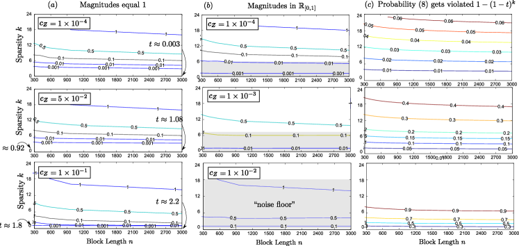
Figure D.1: Empirical LASSO performance shown for $m=150$ for range of $k,n$ values. In $(a)$ the non-zero signal magnitudes $|\alpha_{i}|$ equal 1, and in $(b)$ they are in $\mathbb{R}_{[0,1]}$. In $(c)$ we plot a curve (expression) $1-(1-t)^{k}$ for $t=(3.4+2(1+a))\cdot c_{Z}\sqrt{2\log n}$.

The aim here is to provide more empirical evidence to support observations made in Figure 6 for more block lengths. Here Figure D.1 shows LASSO performance now for a wider range of $n$. We only consider $m=150$, and show various recovery failure rates displayed via contoured lines, for various sparsities $k$ and block lengths $n$. Figures D.1$(a)$ and $(b)$ are companion to Figures 6$(a)$ and $(b)$, in that they respectively correspond to cases where the non-zero signal magnitudes $|\alpha_{i}|$ equal 1 (and $a=0$), and in $\mathbb{R}_{[0,1]}$ (and $a=1$). That is, for $n=1000$, and $k=4$ and $c_{Z}=1\times 10^{-4}$, we see the recovery failure is approximately $1\times 10^{-3}$ in both Figure D.1$(a)$ and Figure 6$(a)$.

As mentioned in Subsection IV-C we observe good empirical match when adjusting the term $t=(a_{1}^{-1}+2a_{3}(1+a))\cdot c_{Z}\sqrt{2\log n}$ (on the RHS of (8)) with $a_{1}=0.29$ and $a_{3}=1$. Figure D.1 provides further support. In $(a)$ we show the values of the term $t$ for values $n=300$ and $n=3000$. Recall in this case when $t>1$ condition (8) (and thus recovery) fails. Observe when $c_{Z}=5\times 10^{-2}$ the values of $t$ are very close to $1$, and for $c_{Z}=1\times 10^{-1}$ they exceed $1$. This matches with our observation in Figure 6$(a)$ that $c_{Z}=5\times 10^{-2}$ is the critical point, beyond which for large $c_{Z}$ recovery fails catastrophically.

In $(b)$ and $(c)$ we look at the other case where $|\alpha_{i}|\in\mathbb{R}_{[0,1]}$. Here $(c)$ plots the probability $1-(1-t)^{k}$ that (8) fails. Again the contoured lines delineate a particular fixed value of $1-(1-t)^{k}$ for various $k,n$ values, whereby we set $t=7.4\cdot c_{Z}\sqrt{2\log n}$ (recall we used $a=1$ here). We observe how closely $(c)$ tracks the noise floor regions in $(b)$ (indicated by shading). More specifically note $t$ really depends on $n$, and the larger the probabilities $1-(1-t)^{k}$ get for various $k,n$ in Figure D.1$(c)$, this probability overwhelms the LASSO recovery rates in Figure D.1$(b)$. This matches with our previous observations in Figure 6$(b)$.

References

- [1] E. Candes and T. Tao, “Decoding by linear programming,” IEEE Trans. on Inform. Theory, vol. 51, pp. 4203–4215, Dec. 2005.
- [2] R. Gribonval and M. Nielsen, “Sparse representations in unions of bases,” IEEE Trans. on Inform. Theory, vol. 49, no. 12, pp. 3320–3325, Dec. 2003.
- [3] D. L. Donoho and M. Elad, “Optimally sparse representation in general (nonorthogonal) dictionaries via minimization,” Proc. of the Nat. Acad. of Sci. (PNAS), vol. 100, no. 5, pp. 2197–2202, Mar. 2003.
- [4] J. A. Tropp, “On the conditioning of random subdictionaries,” Applied and Computational Harmonic Analysis, vol. 25, no. 1, pp. 1–24, Jul. 2008.
- [5] J. J. Fuchs, “On sparse representations in arbitrary redundant bases,” IEEE Trans. on Inform. Theory, vol. 50, no. 6, pp. 1341–1344, Jun. 2004.
- [6] E. Candès and Y. Plan, “Near-ideal model selection by ell_1 minimization,” The Annals of Statistics, vol. 37, no. 5A, pp. 2145–2177, 2009.
- [7] A. Mazumdar and A. Barg, “Sparse recovery properties of statistical RIP matrices,” in IEEE 49th Annual Conf.. on Communication, Control, and Computing (Allerton), Sep. 2011, pp. 9–12.
- [8] Y. Zhang, “Theory of compressive sensing via ell_1-minimization: a non-rip analysis and extensions,” Techical Report, Rice University, 2008.
- [9] A. Cohen, W. Dahmen, and R. DeVore, “Compressed sensing and best k-term approximation,” Journal of the American Mathematical Society, vol. 22, no. 1, pp. 211–231, Jul. 2008.
- [10] A. D’Aspremont and L. El Ghaoui, “Testing the nullspace property using semidefinite programming,” Mathematical Programming, vol. 127, no. 1, pp. 123–144, Mar. 2011.
- [11] D. L. Donoho, “Compressed sensing,” IEEE Trans. on Inform. Theory, vol. 52, no. 4, pp. 1289 – 1306, Apr. 2006.
- [12] R. Baraniuk, M. Davenport, R. DeVore, and M. Wakin, “A simple proof of the restricted isometry property for random matrices,” Constructive Approximation, vol. 28, Dec. 2008.
- [13] J. D. Blanchard, C. Cartis, and J. Tanner, “Compressed sensing: How sharp is the RIP?” SIAM Review, vol. 53, pp. 105–525, Feb. 2011.
- [14] R. Calderbank, S. Howard, and S. Jafarpour, “Construction of a large class of deterministic sensing matrices that satisfy a statistical isometry property,” IEEE Journal of Sel. Topics in Signal Proc., vol. 4, no. 2, pp. 358–374, Apr. 2010.
- [15] L. Gan, C. Long, T. T. Do, and T. D. Tran. (2009) Analysis of the statistical restricted isometry property for deterministic sensing matrices using Stien’s method. [Online]. Available: http://www.dsp.rice.edu/files/cs/Gan_StatRIP.pdf
- [16] M. Sartipi and R. Fletcher, “Energy-Efficient Data Acquisition in Wireless Sensor Networks Using Compressed Sensing,” 2011 Data Compression Conference, pp. 223–232, Mar. 2011.
- [17] F. Chen, A. P. Chandrakasan, and V. Stojanovic, “A signal-agnostic compressed sensing acquisition system for wireless and implantable systems,” in Proceedings of the IEEE Custom Integrated Circuits Conference (CICC ‘10), San Jose, CA, Sep. 2010, pp. 1–4.
- [18] M. Mishali and Y. C. Eldar, “Expected RIP: Conditioning of the modulated wideband converter,” in Proceedings of the IEEE Information Theory Workshop (ITW ‘09), Taormina, Sicily, Oct. 2009, pp. 343–347.
- [19] K. Kanoun, H. Mamaghanian, N. Khaled, and D. Atienza, “A real-time compressed sensing-based personal EKG monitoring system,” in Proceedings of the IEEE/ACM Design, Automation and Test in Europe Conference (DATE ‘11), Grenoble, France, Mar. 2011, pp. 1–6.
- [20] C. Dossal, G. Peyré, and J. Fadili, “A numerical exploration of compressed sampling recovery,” Linear Algebra and its Applications, vol. 432, no. 7, pp. 1663–1679, Mar. 2010.
- [21] B. Bah and J. Tanner, “Improved bounds on restricted isometry constants for gaussian matrices,” SIAM J. Matrix Analysis, vol. 31, no. 5, pp. 2882–2898, 2010.
- [22] D. L. Donoho and J. Tanner, “Neighborliness of randomly-projected simplices in high dimensions,” Proc. of the Nat. Acad. of Sci. (PNAS), vol. 102, pp. 9452–9457, Jul. 2005.
- [23] ——, “Exponential bounds implying construction of compressed sensing matrices, error-correcting codes, and neighborly polytopes by random sampling,” IEEE Trans. on Inform. Theory, vol. 56, no. 4, pp. 2002–2016, Apr. 2010.
- [24] R. Gribnoval, B. Mailhe, H. Rauhut, K. . Schnass, and P. Vandergheynst, “Average case analysis of multichannel thresholding,” in IEEE. International Conference on Acoustics, Speech, and Signal Processing (ICASSP), vol. 2. IEEE, Mar. 2007, pp. II–853–II–856.
- [25] Y. C. Eldar and H. Rauhut, “Average Case Analysis of Multichannel Sparse Recovery Using Convex Relaxation,” IEEE Transactions on Information Theory, vol. 56, no. 1, pp. 1–15, Jan. 2009.
- [26] M. Golbabaee and P. Vandergheynst, “Average case analysis of sparse recovery with thresholding: New bounds based on average dictionary coherence,” in IEEE. International Conference on Acoustics, Speech, and Signal Processing (ICASSP), Mar. 2008, pp. 3877–3880.
- [27] R. Vershynin, “Introduction to the non-asymptotic analysis of random matrices,” in Compressed Sensing, Theory and Applications, Y. Eldar and G. Kutyniok, Eds. Cambridge University Press, 2012, ch. 5, pp. 210–268.
- [28] F. Lim and V. Stojanovic, “On U-statistics and compressed sensing II: Non-asymptotic worst-case analysis,” submitted, 2012.
- [29] E. Candes, “The restricted isometry property and its implications for compressed sensing,” Compte Rendus de l’Academie des Sciences, Paris, Serie I, vol. 336, pp. 589–592, May 2008.
- [30] J. A. Tropp, “Recovery of short, complex linear combinations via minimization,” IEEE Trans. on Inform. Theory, vol. 51, no. 4, pp. 1568–1571, Apr. 2004.
- [31] J. J. Fuchs, “Recovery of exact sparse representations in the presence of bounded noise,” IEEE Transactions on Information Theory, vol. 51, no. 10, pp. 3601–3608, Oct. 2005.
- [32] A. Edelman, “Eigenvalues and condition numbers of random matrices,” SIAM J. Matrix Analysis, vol. 9, no. 4, pp. 543–560, 1988.
- [33] W. Hoeffding, “Probability inequalities for sums of bounded random variables,” J. Am. Stat. Assoc., vol. 58, no. 301, pp. 13–30, Mar. 1963.
- [34] P. K. Sen, “Asymptotic normality of sample quantiles for -dependent processes,” Ann. Math. Statist., vol. 39, no. 5, pp. 1724–1730, 1968.
- [35] P. Koev and A. Edelman, “The efficient evaluation of the hypergoemetric function of a matrix argument,” Mathematics of Computation, vol. 75, no. 254, pp. 833–846, 2006.
- [36] A. Edelman and N. R. Rao, “Random matrix theory,” Acta Numerica, vol. 14, pp. 233–297, May 2005.
- [37] M. Rudelson and R. Vershynin, “Non-asymptotic theory of random matrices : extreme singular values,” in Proceedings of the International Congress of Mathematicians. New Delhi: Hindustan Book Agency, 2010, pp. 1576–1602.
- [38] A. Householder, “The Kantorovich and some related inequalities,” SIAM Review, vol. 7, no. 4, pp. 463–473, 1965.
- [39] R. H. Berk, “Limiting behavior of posterior distribution when the model is incorrect,” Annals of Math. Stat., vol. 37, pp. 51–58, 1966.