Response Function Theory for Many-Body Systems away-from Equilibrium: Conditions of Ultrafast-Time and Ultrasmall-Space Experimental Resolution

Abstract

A Response Function Theory and Scattering Theory applicable to the study of physical properties of systems driven arbitrarily away from equilibrium, specialized for dealing with ultrafast processes and in conditions of space resolution (including nanometric scale), are presented. The derivation is done in the framework of a Gibbs-style Nonequilibrium Statistical Ensemble Formalism. It is shown the connection of the observable properties with time and space-dependent correlation functions out of equilibrium. A generalized fluctuation-dissipation theorem, which relates these correlation functions with generalized susceptibilities is derived. It is also presented the method, useful for calculations, of nonequilibrium-thermodynamic Green functions. A couple of illustration with application of the formalism, consisting of the study of optical responses in ultrafast laser spectroscopy and Raman Scattering of electrons in III-N semiconductors (of ”blue diodes”) driven away from equilibrium by action of electric fields of moderate to high intensities, are described.

I Introduction

The renowned Ryogo Kubo once stated that ”statistical mechanics has been considered a theoretical endeavor. However, statistical mechanics exists for the sake of the real world, not for fictions. Further progress can only be hoped by closed cooperation with experiment” [l]. This is nowadays particularly relevant because the notable development of all the modern technology, fundamental for the progress and well being of the world society, poses a great deal of stress in the realm of basic Physics, more precisely on Thermo-Statistics. Thus, on the one hand, we do face situations in electronics and optoelectronics involving physical-chemical systems far-removed-from equilibrium, where ultrafast (pico- and femto-second scale) and non-linear processes are present. Further, we need to be aware of the rapid unfolding of nano-technologies and use of low-dimensional systems (e.g., nanometric quantum wells and quantum dots in semiconductors heterostructures) [2]. All together this demands having an access to a statistical mechanics being efficient to deal with such requirements. On the other hand, one needs to face the study of soft matter and fluids with complex structures (usually of the average self-affine fractal-like type) [3]. This is relevant for technological improvement in industries like, for example, that of polymers, petroleum, cosmetics, food, electronics and photonics (conducting polymers and glasses), in medical engineering, etc. Moreover, in both type of situations above mentioned there often appear difficulties of description and objectivity (existence of so-called ”hidden constraints”), which impair the proper application of the conventional ensemble approach used in the general, logically and physically sound, and well established Boltzmann-Gibbs statistics. A tentative to partially overcome such difficulties consists into resorting to non-conventional approaches [4-7].

Since, as noticed, a most relevant objective of any nonequilibrium statistical theory is to provide a comprehension of the underlying physics related to the relaxation phenomena that can be evidenced in experiments, it needs be coupled with a response function theory. This is the subject of this paper, where we specifically resort to the use of a Non-Equilibrium Statistical Ensemble Formalism (NESEF for short) [8-11]).

It can be noticed that nowadays two approaches appear to be the most favorable for providing very satisfactory methods to deal with systems within an ample scope of nonequilibrium conditions. They are, on the one hand, Numerical Simulation Methods [12], or Computational Physics. In particular, to it belongs Non-Equilibrium Molecular-dynamics NMD [13], a computational method created for modeling physical systems at the microscopic level, being a good technique to study the molecular behavior of several physical processes. On the other hand, we do have the kinetic theory based on the far-reaching generalization of Gibbs’ ensemble formalism, the NESEF [11,14].

The present structure of the formalism consists in an extension and generalization of earlier pioneering approaches, among which we can pinpoint the works of Kirkwood [15], Green [16], Mori-Oppenheim-Ross [17], Mori [18] and Zwanzig [19]. NESEF has been approached from different points of view: some are based on heuristic arguments, others on projection-operator techniques (the former following Kirkwood and Green and the latter following Zwanzig and Mori).

The formalism has been systematized and largely improved by the Russian School of statistical physics, which can be considered to have been initiated by the renowned Nicolai Nicolaievich Bogoliubov (e.g., see ref. [20]) and we may also name Nicolai Sergeievich Krylov [21], and more recent1y mainly through the relevant contributions of Dimitrii Zubarev [8,9], Sergei Peletminskii [22], and others. We present in Refs. [11] a systematization, as well as generalizations and conceptual discussions, of the matter.

It may be noticed that these different approaches to NESEF can be brought together under a unique variational principle. This has been originally done by Zubarev and Kalashnikov [23] and later on reconsidered in Refs. [9,11]. It consists on the maximization, in the context of information Theory, of Gibbs statistical entropy (that is, the average of minus the logarithm of the statistical distribution function [24,25], which in Communication Theory is Shannon informational entropy [26,27], subjected to certain constraints and including non-locality in space, retro-effects, and irreversibility on the macroscopic level.

Concerning Response Function Theory, the usual theory to calculate linear responses to mechanical perturbations (e.g. [28-33]) is based on expansions in terms of correlation functions in equilibrium. As initial condition is taken that of equilibrium with a thermal reservoir, and next it is studied the evolution of the system as if it were isolated from all external influences except the driving field. Let us now consider the situation when a mechanical perturbation is applied on an already far-from-equilibrium system, in which are unfolding irreversible processes which are describable in terms of equations of evolution for a basic set of macrovariables in the non-equilibrium thermodynamic space of states. Since NESEF provides a seemingly powerful method to obtain a description of the macrostate of such systems, it is appealing to derive a response function theory based on correlation functions in the unperturbed nonequilibrium state of the system. Schemes of this type have been proposed [31-33], and next we systematize and extend this treatment, in such a way to allow the treatment of experiments involving time-resolution (including the ultrafast time scale of pico- and femto-seconds), and space resolution (including those in the emerging nano-science and technology).

It is shown the connection of the observable properties with correlation functions out of equilibrium; a generalized fluctuation-dissipation theorem – relating correlation functions and generalized susceptibilities – is derived, and the method, useful for calculations, of nonequilibrium-thermodynamic Green functions is presented. This is done in Sections II, III and IV, and in Section V we present a scattering theory, in the same conditions, namely, including time and space resolution, for systems far-from equilibrium. The connection of the scattering theory with response function theory follows from application of the nonequilibrium fluctuation-dissipation theorem.

Finally, in Section VI we present a couple of illustrations showing the working of the theory in the study of two kind of experiments, namely optical responses in ultrafast laser spectroscopy of polar semiconductors, and Raman scattering of electrons in doped III-N semiconductors (”blue diodes”) in the presence of electric fields with moderate to high intensities. In the latter case the nonequilibrium fluctuation-dissipation theorem allows to connect the Raman spectrum with nonlinear transport properties in these materials (nonlinear and time-dependent conductivity and diffusion coefficient, and a generalized - nonlinear and time-dependent Einstein-relation).

II Response Function Theory for Far-From-Equilibrium Systems

We consider an open many-body system out of equilibrium, which is in contact with a set of reservoirs and under the action of pumping sources. We are essentially presenting the most general experiment one can think of, namely a sample (the open system of interest composed of very-many degrees of freedom) subjected to given experimental conditions, as it is diagrammatically described in Fig. 1.

Figure 1: Diagrammatic description of a typical pump-probe experiment in an open dissipative system.

In Fig. 1, the sample is composed of a number of subsystems, $\sigma_{j}$, (or better to say subdegrees of freedom, for example, in solid state matter those associated to electrons, lattice vibrations, excitons, impurity states, collective excitations as plasmons, magnons, etc., hybrid excitations as polarons, polaritons, plasmaritons and so on). They interact among themselves via interaction potentials producing exchange at certain rates, $\tau_{ij}$, of energy and momentum. Pumping sources act on the different subsystems of the sample – via particular types of fields, electric, magnetic, electromagnetic, etc. – well characterized when setting up the experiment, and there follows relaxation of the energy in excess of equilibrium the system is receiving to the external reservoirs, $\tau_{jR}$. Finally, the experiment is performed coupling an external probing source, characterized in the figure by $P(t)$, with one or more subsystems of the sample, and some kind of response, say $R(t)$, is detected by a measuring apparatus (e.g. ammeter, spectrometer, etc.).

It needs be understood that the pumping sources exert their influence on the given open system through the fields they generate, say, magnetic, electric, electromagnetic as produced for example from a laser machine, and so on, or, eventually, in scattering experiments is the interaction potential with the particles of an incoming beam.

Let the Hamiltonian be

$$\hat{H}(t)=\hat{H}_{\sigma}+\hat{\mathcal{V}}(t)\;,$$ (1)

that is, the Hamiltonian $\hat{H}_{\sigma}$ of the system in the presence of the fields of the pumping sources which drive it away from equilibrium, plus the interactions with the reservoirs, and with the field(s), $\hat{\mathcal{V}}(t)$, created by the external perturbing apparatus. We take for the latter the form

$$\hat{\mathcal{V}}(t)=-\int d^{3}r^{\prime}\,\mathcal{F}(\mathbf{r}^{\prime},t)\hat{A}(\mathbf{r}^{\prime})\;,$$ (2)

where $\mathcal{F}$ is the expression for the perturbing force ($\mathcal{F}=-\delta\hat{\mathcal{V}}/\delta\hat{A}(\mathbf{r}^{\prime})$, where $\delta$ is a functional derivative) and $\hat{A}(\mathbf{r}^{\prime})$ an observable of the system to which it is coupled. We recall that the system is in contact with ideal reservoirs, and the statistical operator is taken as a product of the one of the system $\varrho_{\varepsilon}(t)$ times the stationary canonical distribution of the reservoirs $\varrho_{R}$, which we write $\mathcal{R}_{\varepsilon}(t)=\varrho_{\varepsilon}(t)\times\varrho_{R}$ [11] (see Appendix A). Moreover, $\hat{H}_{\sigma}=\hat{H}_{0}+\hat{H}_{1}+\hat{W}=\hat{H}_{0}+\hat{H}^{\prime}$, introducing $\hat{H}^{\prime}=\hat{H}_{1}+\hat{W}$, where $H_{1}$ accounts for all the interactions in the system and $W$ for the interaction with the surroundings.

Schrödinger equation for this system, i.e.

$$i\hbar\frac{\partial}{\partial t}|\psi(t)\rangle=\hat{H}(t)|\psi(t)\rangle\;,$$ (3)

with the initial condition $|\psi(t_{i})\rangle$ at time $t_{i}$ when the perturbation is switched on, has the formal solution

$$|\psi(t)\rangle=U(t,t_{i})|\psi(t_{i})\rangle\;,$$ (4)

where $U$ is the evolution operator satisfying that

$$i\hbar\frac{\partial}{\partial t}U(t,t_{i})=\hat{H}(t)U(t,t_{i})\;,$$ (5)

with $U(t_{i},t_{i})=\hat{1}$ (the unit operator), and we recall that it is a unitary operator, that is $U^{\dagger}U=\hat{1}$.

Let us now introduce the interaction representation, writing

$$U(t,t_{i})=U_{\sigma}(t,t_{i})U^{\prime}(t,t_{i})\;,$$ (6)

where

$$U_{\sigma}(t,t_{i})=\exp\Biggl{\{}\frac{1}{i\hbar}(t-t_{i})\hat{H}_{\sigma}\Biggr{\}}\;,$$ (7)

which is the evolution operator in the absence of the perturbation potential $\hat{\mathcal{V}}$; this means that we are separating the internal dynamics of the system from the dynamical effects of the perturbation which are accounted for by $U^{\prime}$. Introducing Eq. (6) in Eq. (5) and using Eq. (7), it follows that $U^{\prime}$ satisfies the equation

$$i\hbar\frac{\partial}{\partial t}U^{\prime}(t,t_{i})=\tilde{\mathcal{V}}(t)U^{\prime}(t,t_{i})\;,$$ (8)

with $U^{\prime}(t_{i},t_{i})=\hat{1}$, and

$$\tilde{\mathcal{V}}(t)=U_{\sigma}^{\dagger}(t,t_{i})\hat{\mathcal{V}}(t)U_{\sigma}(t,t_{i})\;.$$ (9)

Equation (8) can be transformed in an equivalent integral equation, namely

$$U^{\prime}(t,t_{i})=\hat{1}+\frac{1}{i\hbar}\int_{t_{i}}^{t}dt^{\prime}\,\tilde{\mathcal{V}}(t^{\prime})U^{\prime}(t^{\prime},t_{i})\;,$$ (10)

which admits the iterated solution

$$U^{\prime}(t,t_{i}) = \hat{1}+\frac{1}{i\hbar}\int_{t_{i}}^{t}dt^{\prime}\,\tilde{\mathcal{V}}(t^{\prime})+\frac{1}{(i\hbar)^{2}}\int_{t_{i}}^{t}dt^{\prime}\int_{t_{i}}^{t^{\prime}}dt^{\prime\prime}\,\tilde{\mathcal{V}}(t^{\prime})\tilde{\mathcal{V}}(t^{\prime\prime})+\cdots$$ (11)

$$= \hat{1}+\sum_{n=1}^{\infty}\frac{1}{(i\hbar)^{n}}\int_{t_{i}}^{t}dt_{1}\cdots\int_{t_{i}}^{t_{n-1}}dt_{n}\,\tilde{\mathcal{V}}(t_{1})\cdots\tilde{\mathcal{V}}(t_{n})\;.$$

The quantum-mechanical expected value at time $t$ of the observable $\hat{A}(\mathbf{r})$, to which the external field is coupled, is then

$$a(\mathbf{r},t) = \langle\psi(t)|\hat{A}(\mathbf{r})|\psi(t)\rangle$$ (12)

$$= \langle\psi(t_{i})|{U^{\prime}}^{\dagger}(t,t_{i})U_{\sigma}^{\dagger}(t,t_{i})\hat{A}(\mathbf{r})U_{\sigma}(t,t_{i})U^{\prime}(t,t_{i})|\psi(t_{i})\rangle$$

$$= \langle\psi(t_{i})|{U^{\prime}}^{\dagger}(t,t_{i})\tilde{A}(\mathbf{r},t)U^{\prime}(t,t_{i})|\psi(t_{i})\rangle\;,$$

where

$$\tilde{A}(\mathbf{r},t)=U_{\sigma}^{\dagger}(t,t_{i})\hat{A}(\mathbf{r})U_{\sigma}(t,t_{i})\;.$$ (13)

According to Eq. (11) we have that

$$a(\mathbf{r},t) = \langle\psi(t_{i})|(\hat{1}-\frac{1}{i\hbar}\int_{t_{i}}^{t}dt^{\prime}\,\tilde{\mathcal{V}}(t^{\prime})+\cdots)\tilde{A}(\mathbf{r},t)\times$$ (14)

$$(\hat{1}+\frac{1}{i\hbar}\int_{t_{i}}^{t}dt^{\prime}\,\tilde{\mathcal{V}}(t^{\prime})+\cdots)|\psi(t_{i})\rangle\;,$$

where we have used that $\tilde{\mathcal{V}}$ is Hermitian.

Considering a weak perturbation – characterized by $\hat{\mathcal{V}}(t)$ – imposed on the initially (at time $t_{i}$) far-from-equilibrium system, we truncate the series of terms in Eq. (14) in first order in $\tilde{\mathcal{V}}$, that is, we consider from now on a linear response theory, to obtain that

$$a(\mathbf{r},t)=a(\mathbf{r},t_{i})+\frac{1}{i\hbar}\int_{t_{i}}^{t}dt^{\prime}\,\langle\psi(t_{i})|[\tilde{A}(\mathbf{r},t),\tilde{\mathcal{V}}(t^{\prime})]|\psi(t_{i})\rangle\;,$$ (15)

where

$$a(\mathbf{r},t_{i})=\langle\psi(t_{i})|\hat{A}(\mathbf{r})|\psi(t_{i})\rangle$$ (16)

is the expected value of the observable at time $t_{i}$ prior to the application of the perturbation.

Using Eq. (2) we have that

$$\Delta a(\mathbf{r},t)=-\frac{1}{i\hbar}\int_{t_{i}}^{t}dt^{\prime}\int d^{3}r^{\prime}\,\langle\psi(t_{i})|[\tilde{A}(\mathbf{r},t),\tilde{A}(\mathbf{r}^{\prime},t^{\prime})]\mathcal{F}(\mathbf{r}^{\prime},t^{\prime})|\psi(t_{i})\rangle\;,$$ (17)

where $\Delta a(\mathbf{r},t)=a(\mathbf{r},t)-a(\mathbf{r},t_{i})$ is the departure of the observable $\hat{A}$ from its value at the initial time when under the action of the perturbing potential.

Introducing the statistical operator for the pure (quantum mechanical) state, namely

$$\mathcal{P}(t_{i})=|\psi(t_{i})\rangle\langle\psi(t_{i})|\;,$$ (18)

which, we recall, is a projection operator over the vector state $|\psi(t_{i})\rangle$, we can rewrite Eq. (17) as

$$\Delta a(\mathbf{r},t)=-\frac{1}{i\hbar}\int_{-\infty}^{t}dt^{\prime}\int d^{3}r^{\prime}\,Tr\{[\tilde{A}(\mathbf{r},t),\tilde{A}(\mathbf{r}^{\prime},t^{\prime})]\mathcal{P}(t_{i})\}\mathcal{F}(\mathbf{r}^{\prime},t^{\prime})\;,$$ (19)

and where we have considered adiabatic application of the perturbation taken as $t_{i}\rightarrow-\infty$.

Next step is going over the macroscopic state taking the average over the nonequilibrium ensemble of pure states, compatible with the macroscopic conditions of preparation of the sample. In the usual way, if we call $\mathcal{P}_{n}(t_{i})$ the statistical operator for the pure state in, say, the $n$-th replica, and $p_{n}$ the probability of such replica in the corresponding Gibbs ensemble, the statistical average over the ensemble of mixed states of the system, and the average over the states of the reservoir (system and reservoir are coupled via the interaction $\hat{W}$) is

$$\Delta\langle\hat{A}(\mathbf{r})|t\rangle = -\frac{1}{i\hbar}\int_{-\infty}^{t}\!\!dt^{\prime}\int\!d^{3}r^{\prime}\sum_{n}p_{n}\times$$ (20)

$$Tr\bigl{\{}[\tilde{A}(\mathbf{r},t),\tilde{A}(\mathbf{r}^{\prime},t^{\prime})]\mathcal{P}_{n}(t_{i})\times\varrho_{R}\bigr{\}}\mathcal{F}(\mathbf{r}^{\prime},t^{\prime})$$

$$= -\frac{1}{i\hbar}\int_{-\infty}^{t}dt^{\prime}\int d^{3}r^{\prime}\,Tr\{[\tilde{A}(\mathbf{r},t),\tilde{A}(\mathbf{r}^{\prime},t^{\prime})]\varrho_{\varepsilon}(t_{i})\times\varrho_{R}\}\mathcal{F}(\mathbf{r}^{\prime},t^{\prime})\;,$$

with

$$\varrho_{\epsilon}(t_{i})=\sum_{n}p_{n}\mathcal{P}_{n}(t_{i})=\sum_{n}p_{n}|\psi_{n}(t_{i})\rangle\langle\psi_{n}(t_{i})|\;,$$ (21)

and we have introduced

$$\Delta\langle\hat{A}(\mathbf{r})|t\rangle=Tr\{\hat{A}(\mathbf{r})\mathcal{R}_{\varepsilon}(t)\}-Tr\{\hat{A}(\mathbf{r})\mathcal{R}_{\varepsilon}(t_{i})\}\;,$$ (22)

where, we recall, $\mathcal{R}_{\varepsilon}(t)=\varrho_{\varepsilon}(t)\times\varrho_{R}$.

But Eq. (20) can be rewritten as

$$\Delta\langle\hat{A}(\mathbf{r})|t\rangle=-\frac{1}{i\hbar}\int_{-\infty}^{t}dt^{\prime}\int d^{3}r,Tr\bigl{\{}[\tilde{A}(\mathbf{r}),\tilde{A}(\mathbf{r}^{\prime},t^{\prime}-t)]\mathcal{R}_{\varepsilon}(t)\bigr{\}}\mathcal{F}(\mathbf{r}^{\prime},t^{\prime})\;,$$ (23)

since

$$Tr\{[U_{\sigma}^{\dagger}(t,t_{i})\hat{A}(\mathbf{r})U_{\sigma}(t,t_{i}),U_{\sigma}^{\dagger}(t^{\prime},t_{i})\hat{A}(\mathbf{r}^{\prime})U_{\sigma}(t^{\prime},t_{i})]\mathcal{R}_{\varepsilon}(t_{i})\}=\\ Tr\{\tilde{A}(\mathbf{r}),\tilde{A}(\mathbf{r}^{\prime},t^{\prime}-t)\mathcal{R}_{\varepsilon}(t)\}\;,$$ (24)

where we have used the invariance of the trace operation by cyclical permutations and the group properties of operators $U$. We stress that in nonequilibrium conditions there is no invariance for translation in time as a result of the time-dependence of the statistical operator which describes the irreversible evolution of the macroscopic state; the operator $A(t^{\prime}-t)$ in Eq. (24) shows time-translational invariance because such dependence on time arises out of the microdynamical evolution governed by Hamiltonian $H_{\sigma}$.

Moreover, introducing the definitions

$$\chi^{\prime\prime}(\mathbf{r},\mathbf{r}^{\prime};t^{\prime}-t|t)=\frac{1}{2\hbar}Tr\{[\hat{A}(\mathbf{r}),\tilde{A}(\mathbf{r}^{\prime},t^{\prime}-t)]\mathcal{R}_{\varepsilon}(t)\}\;,$$ (25)

$$\chi(\mathbf{r},\mathbf{r}^{\prime};t-t^{\prime}|t)=2i\theta(t-t^{\prime})\chi^{\prime\prime}(\mathbf{r},\mathbf{r}^{\prime};t^{\prime}-t|t)\;,$$ (26)

with $\theta$ being Heaviside’s step function, we have that Eq. (20) becomes

$$\Delta\langle\hat{A}(\mathbf{r})|t\rangle=\int_{-\infty}^{\infty}dt^{\prime}\int d^{3}r^{\prime}\,\chi(\mathbf{r},\mathbf{r}^{\prime};t-t^{\prime}|t)\mathcal{F}(\mathbf{r}^{\prime},t^{\prime})\;.$$ (27)

Taking into account the integral representation of Heaviside step function, namely

$$\theta(\tau)=\lim_{s\rightarrow+\!0}\;i\int_{-\infty}^{\infty}\frac{d\omega}{2\pi}\frac{e^{-i\omega\tau}}{\omega+is}\;,$$ (28)

we find, after some calculus, that the Fourier transform in time $\tau=t-t^{\prime}$ of the nonequilibrium generalized susceptibility of Eq. (26) is given by

$$\chi(\mathbf{r},\mathbf{r}^{\prime};\omega|t)=\int_{-\infty}^{\infty}\frac{d\omega^{\prime}}{\pi}\frac{\chi^{\prime\prime}(\mathbf{r},\mathbf{r}^{\prime};\omega^{\prime}|t)}{\omega^{\prime}-\omega-is}\;,$$ (29)

where, we recall, $s\rightarrow+\!0$, and $\chi^{\prime\prime}(\mathbf{r},\mathbf{r}^{\prime};\omega^{\prime}|t)$ is the Fourier transform at frequency $\omega$ of the $\tau$-dependent $\chi^{\prime\prime}$ of Eq. (25), namely

$$\chi^{\prime\prime}(\mathbf{r},\mathbf{r}^{\prime};\omega|t)=\int_{-\infty}^{\infty}d\tau\,\chi^{\prime\prime}(\mathbf{r},\mathbf{r}^{\prime};-\tau|t)e^{i\omega\tau}\;.$$ (30)

Using the fact that

$$\lim_{s\rightarrow+\!0}\frac{1}{x\pm is}=pv\frac{1}{x}\mp i\pi\delta(x)\;,$$ (31)

which are the so-called advanced and retarded Heisenberg delta functions and $pv$ stands for principal value, Eq. (29) becomes

$$\chi(\mathbf{r},\mathbf{r}^{\prime};\omega|t) = Re\{\chi(\mathbf{r},\mathbf{r}^{\prime};\omega|t)\}+iIm\{\chi(\mathbf{r},\mathbf{r}^{\prime};\omega|t)\}$$ (32)

$$= pv\int_{-\infty}^{\infty}\frac{d\omega^{\prime}}{\pi}\frac{\chi^{\prime\prime}(\mathbf{r},\mathbf{r}^{\prime};\omega^{\prime}|t)}{\omega^{\prime}-\omega}+i\chi^{\prime\prime}(\mathbf{r},\mathbf{r}^{\prime};\omega|t)\;,$$

where $Re$ and $Im$ stand for real and imaginary parts respectively, and then

$$Im\chi(\mathbf{r},\mathbf{r}^{\prime};\omega|t)=\chi^{\prime\prime}(\mathbf{r},\mathbf{r}^{\prime};\omega|t)\;,$$ (33)

$$Re\chi(\mathbf{r},\mathbf{r}^{\prime};\omega|t)=pv\int_{-\infty}^{\infty}\frac{d\omega^{\prime}}{\pi}\frac{Im\chi(\mathbf{r},\mathbf{r}^{\prime};\omega^{\prime}|t)}{\omega^{\prime}-\omega}\;,$$ (34)

after recalling that $\chi^{\prime\prime}(\mathbf{r},\mathbf{r}^{\prime};\omega|t)$ is a real quantity as shown in Eq. (51).

This Eq. (34) is one of the so-called generalized Kramer-Krönig relations, with the other being

$$Im\chi(\mathbf{r},\mathbf{r}^{\prime};\omega|t)=-pv\int_{-\infty}^{\infty}\frac{d\omega^{\prime}}{\pi}\frac{Re\chi(\mathbf{r},\mathbf{r}^{\prime};\omega^{\prime}|t)}{\omega^{\prime}-\omega}\;,$$ (35)

obtained from Eq. (34) once it is used the operational relation

$$pv\int_{-\infty}^{\infty}\frac{d\omega^{\prime\prime}}{\pi}(\omega-\omega^{\prime\prime})^{-1}(\omega^{\prime\prime}-\omega^{\prime})^{-1}=-\pi\delta(\omega-\omega^{\prime})\;.$$ (36)

We recall that Kramer-Krönig relations are a consequence of the principle of causality, and involving the fact that $\chi$, once extended to the complex $z$-plane ($z=\omega+iy$), i.e. $\chi(\mathbf{r},\mathbf{r}^{\prime};z|t)$, has poles in the lower $z$-plane and it is regular in the upper $z$-plane. Furthermore we notice that $Re\chi$ is an even function of $\omega$ while $Im\chi$ is an odd one. Thus, $\chi(\mathbf{r},\mathbf{r}^{\prime};\omega|t)$ has the same properties as the equilibrium one presented in Eq. (52) below, as it should.

Moreover, $Im\chi(\mathbf{r},\mathbf{r}^{\prime};\omega|t)$ is related to the power absorption by the system. First, we notice that the external force applied on the system can be Fourier analyzed in time, obtaining a linear superposition of Fourier components, namely

$$\mathcal{F}(\mathbf{r}^{\prime},t^{\prime})=\int d\omega\frac{1}{2}\mathcal{F}(\mathbf{r}^{\prime},\omega)(e^{i\omega t^{\prime}}+e^{-i\omega t^{\prime}})\;,$$ (37)

so it is a real quantity, and let us calculate the average over time $t^{\prime}$ (and then $\tau$) of the quantity which represents the power absorbed by the system, namely the average over a time interval $\Delta t$ (typically the experimental resolution time) given by

$$W(t) = \frac{1}{\Delta t}\int_{t}^{t+\Delta t}dt^{\prime}\,\frac{dE(t^{\prime})}{dt^{\prime}}=\frac{1}{\Delta t}\int_{t}^{t+\Delta t}dt^{\prime}\,\frac{d}{dt^{\prime}}Tr\{\hat{H}(t^{\prime})\mathcal{R}_{\varepsilon}(t^{\prime})\}$$ (38)

$$= \frac{1}{\Delta t}\int_{t}^{t+\Delta t}dt^{\prime}Tr\Biggl{\{}\frac{\partial\hat{H}(t^{\prime})}{\partial t^{\prime}}\mathcal{R}_{\varepsilon}(t^{\prime})+\hat{H}(t^{\prime})\frac{\partial}{\partial t^{\prime}}\mathcal{R}_{\varepsilon}(t^{\prime})\Biggr{\}}\;,$$

But, we do have that

$$Tr\Bigl{\{}\hat{H}(t^{\prime})\frac{\partial}{\partial t^{\prime}}\mathcal{R}_{\varepsilon}(t^{\prime})\Bigr{\}}=\frac{1}{i\hbar}Tr\bigl{\{}[\hat{H}(t^{\prime}),\hat{H}(t^{\prime})]\mathcal{R}_{\varepsilon}(t^{\prime})\bigr{\}}=0\;,$$ (39)

where we have used that $\mathcal{R}_{\varepsilon}$ satisfies Liouville equation. Hence

$$W(t) = \frac{1}{\Delta t}\int_{t}^{t+\Delta t}dt^{\prime}\,Tr\Bigl{\{}\frac{\partial\hat{H}(t^{\prime})}{\partial t^{\prime}}\mathcal{R}_{\varepsilon}(t^{\prime})\Bigr{\}}$$ (40)

$$= \frac{1}{\Delta t}\int_{t}^{t+\Delta t}dt^{\prime}\,Tr\Bigl{\{}\frac{\partial\hat{\mathcal{V}}(t^{\prime})}{\partial t^{\prime}}\mathcal{R}_{\varepsilon}(t^{\prime})\Bigr{\}}$$

$$= -\frac{1}{\Delta t}\int_{t}^{t+\Delta t}dt^{\prime}\int d^{3}r^{\prime}Tr\{\hat{A}(\mathbf{r}^{\prime})\mathcal{R}_{\varepsilon}(t^{\prime})\}\frac{\partial\mathcal{F}(\mathbf{r}^{\prime},t^{\prime})}{\partial t^{\prime}}\;,$$

with $\hat{\mathcal{V}}$ given in Eq. (2). Taking into account that

$$Tr\{\hat{A}(\mathbf{r}^{\prime})\mathcal{R}_{\varepsilon}(t)\} = Tr\{\hat{A}(\mathbf{r}^{\prime})U(t^{\prime},t_{i})\mathcal{R}_{\varepsilon}(t_{i})U^{\dagger}(t^{\prime},t_{i})\}$$ (41)

$$= Tr\{U^{\dagger}(t^{\prime},t_{i})\hat{A}(\mathbf{r}^{\prime})U(t^{\prime},t_{i})\mathcal{R}_{\varepsilon}(t_{i})\}$$

$$= Tr\{{U^{\prime}}^{\dagger}(t^{\prime},t_{i})\tilde{A}(\mathbf{r}^{\prime},t^{\prime})U^{\prime}(t^{\prime},t_{i})\mathcal{R}_{\varepsilon}(t_{i})\}\;,$$

where we used Eqs. (6) and (13), and next, resorting to Eq. (11) in first order (linear response) and to Eq. (20), we find that

$$W(t) = \frac{1}{i\hbar\Delta t}\int_{t}^{t+\Delta t}dt^{\prime}\int d^{3}r^{\prime}\int_{-\infty}^{t^{\prime}}dt^{\prime\prime}\int d^{3}r^{\prime\prime}\,Tr\{[\tilde{A}(\mathbf{r}^{\prime},t^{\prime}),\tilde{A}(\mathbf{r}^{\prime\prime},t^{\prime\prime})]\times$$ (42)

$$\mathcal{R}_{\varepsilon}(t_{i})\}\mathcal{F}(\mathbf{r}^{\prime\prime},t^{\prime\prime})\frac{\partial\mathcal{F}(\mathbf{r}^{\prime},t^{\prime})}{\partial t^{\prime}}$$

$$= -\frac{1}{\Delta t}\!\int_{t}^{t+\Delta t}\!\!dt^{\prime}\!\int\!d^{3}r^{\prime}\,\Delta A(\mathbf{r}^{\prime},t^{\prime})\frac{\partial\mathcal{F}(\mathbf{r}^{\prime},t^{\prime})}{\partial t^{\prime}}\;,$$

with $\Delta A$ of Eq. (20). Because of Eq. (27) we can write Eq. (42) in the alternative form

$$W(t) = -\frac{1}{\Delta t}\int_{t}^{t+\Delta t}dt^{\prime}\int d^{3}r^{\prime}\int d^{3}r^{\prime\prime}\int_{-\infty}^{\infty}d\tau\,\chi(\mathbf{r}^{\prime},\mathbf{r}^{\prime\prime};\tau|t^{\prime})\times$$ (43)

$$\mathcal{F}(\mathbf{r}^{\prime\prime},\tau+t^{\prime})\frac{\partial\mathcal{F}(\mathbf{r}^{\prime},t^{\prime})}{\partial t^{\prime}}\;,$$

with $\tau=t^{\prime\prime}-t^{\prime}$, and using Eq. (37) and the Fourier transform of $\chi$, it follows

$$W(t) = -\frac{1}{\Delta t}\int_{t}^{t+\Delta t}dt^{\prime}\int d^{3}r^{\prime}\int d^{3}r^{\prime\prime}\,\int d\omega i\omega\mathcal{F}(\mathbf{r}^{\prime\prime},\omega)\mathcal{F}(\mathbf{r}^{\prime},\omega)\times$$ (44)

$$\Bigl{\{}\chi^{\ast}(\mathbf{r}^{\prime},\mathbf{r}^{\prime\prime};\omega|t^{\prime})(e^{2i\omega t^{\prime}}-1)-\chi(\mathbf{r}^{\prime},\mathbf{r}^{\prime\prime};\omega|t^{\prime})(e^{-2i\omega t^{\prime}}-1)\Bigr{\}}\;.$$

If we consider a particular situation in which $\mathcal{R}_{\varepsilon}(t^{\prime})$ varies weakly in time in the interval $\Delta t$ (implying in that ultrafast relaxation processes are not present), we can approximate it by $\mathcal{R}_{\varepsilon}(t)$, and in conditions such that $\Delta t$ involves several periods $2\pi/\omega$ so that the exponentials cancel on average, using Eq. (23) it follows that

$$W(t)=\frac{1}{2}\int d^{3}r^{\prime}\int d^{3}r^{\prime\prime}\int d\omega\mathcal{F}(\mathbf{r}^{\prime},\omega)\mathcal{F}(\mathbf{r}^{\prime\prime},\omega)\alpha(\mathbf{r}^{\prime},\mathbf{r}^{\prime\prime};\omega|t)\;,$$ (45)

where

$$\alpha(\mathbf{r}^{\prime},\mathbf{r}^{\prime\prime};\omega|t)=\omega\chi^{\prime\prime}(\mathbf{r}^{\prime},\mathbf{r}^{\prime\prime};\omega|t)$$ (46)

can be considered a kind of absorption coefficient at each frequency $\omega$ associated to the perturbing force, and at the macroscopic (nonequilibrium thermodynamic) state of the system at time $t$.

Evidently, and this is a fundamental point to be stressed, the generalized susceptibility depends on $\varrho_{\varepsilon}$, through $\mathcal{R}_{\varepsilon}$, and since the latter is a functional of the time- (and eventually of the space-) dependent variables that characterized the nonequilibrium thermodynamic state of the system, then the calculus of responses needs be coupled with the one of the equations of evolution for the basic variables, as given by the nonlinear quantum kinetic theory that the formalism provides [8-11,14].

Closing this section let us add some additional considerations.

First, if the system has translational invariance (or near translational invariance as in the case of regular crystalline matter), the dependence of $\chi^{\prime\prime}$ and $\chi$ on $\mathbf{r}$ and $\mathbf{r}^{\prime}$ is through the difference $\mathbf{r}-\mathbf{r}^{\prime}$. We can then introduce the Fourier transform in space, namely

$$\chi^{\prime\prime}(\mathbf{k},\omega|t)=\int d^{3}b\,\chi^{\prime\prime}(b,\omega|t)e^{-i\mathbf{k}\cdot\mathbf{b}}\;,$$ (47)

where $\mathbf{b}=\mathbf{r}-\mathbf{r}^{\prime}$. Moreover,

$$[\chi^{\prime\prime}(\mathbf{r},\mathbf{r}^{\prime};-\tau|t)]^{\ast}=-\chi^{\prime\prime}(\mathbf{r},\mathbf{r}^{\prime};-\tau|t)\;,$$ (48)

as a result of $\chi^{\prime\prime}$ involving a commutator of Hermitian operators, and this $\chi^{\prime\prime}$ is then a purely imaginary quantity. Similarly, it follows that

$$\chi^{\prime\prime}(\mathbf{r},\mathbf{r}^{\prime};-\tau|t)=-\chi^{\prime\prime}(\mathbf{r},\mathbf{r}^{\prime};\tau|t)\;,$$ (49)

what implies that

$$\chi^{\prime\prime}(\mathbf{k},\omega|t)=-\chi^{\prime\prime}(-\mathbf{k},-\omega|t)\;.$$ (50)

On the other hand, on the basis of Eqs. (32) and (50) we have that

$$Im\,\chi(\mathbf{k},\omega|t) = \frac{1}{2i}\bigl{(}\ \chi(\mathbf{k},\omega|t)-\chi^{\ast}(\mathbf{k},\omega|t)\bigr{)}$$ (51)

$$= \frac{1}{2i}\int_{-\infty}^{\infty}\frac{d\omega}{\pi}\int d^{3}b\int d\tau\,\chi^{\prime\prime}(\mathbf{b},-\tau|t)\left(\frac{e^{-i(\mathbf{k}\cdot\mathbf{b}-\omega^{\prime}\tau)}}{\omega^{\prime}-\omega-is}+\frac{e^{i(\mathbf{k}\cdot\mathbf{b}-\omega^{\prime}\tau)}}{\omega^{\prime}-\omega+is}\right)\hfill$$

$$= \frac{1}{2i}\int_{-\infty}^{\infty}\frac{d\omega}{\pi}\int d^{3}b\int d\tau\,e^{-i(\mathbf{k}\cdot\mathbf{b}-\omega\tau)}\left(\frac{\chi^{\prime\prime}(\mathbf{b},-\tau|t)}{\omega^{\prime}-\omega-is}+\frac{\chi^{\prime\prime}(-\mathbf{b},\tau|t)}{\omega^{\prime}-\omega+is}\right)\hfill$$

$$= \chi^{\prime\prime}(\mathbf{k},\omega|t)\,,$$

which is then a real quantity, and also is $\chi^{\prime\prime}(\mathbf{r},\mathbf{r}^{\prime};\omega|t)$.

Moreover, if the initial condition of preparation of the system is the one of equilibrium with the reservoirs, characterized by distribution $\varrho_{\text{eq}}$ (which commutes with $\hat{H}$), we recover the usual expression [28]

$$\chi(\mathbf{r},\mathbf{r}^{\prime};t-t^{\prime})_{\text{eq}}=\theta(t-t^{\prime})\frac{i}{\hbar}Tr\bigl{\{}[\hat{A}(\mathbf{r}),\tilde{A}(\mathbf{r}^{\prime},t^{\prime}-t)]\,\varrho_{\text{eq}}\bigr{\}}\;.$$ (52)

where, as usual, because the equilibrium has been established, the interaction of system and reservoir is neglected.

Secondly, as pointed out in the Introduction the notable developments in instrumentation that are at present being accumulated, and which are necessary for the study of systems working in far-from-nonequilibrium conditions in the sought-after miniaturized devices with ultrafast responses of nowadays advanced technology, require the mechanical-statistical analysis in short time intervals (as described above) and in nanometric spatial regions. This is also contained in the theoretical treatment already described. In fact, if the property of the systems is measured in a small region around position $\mathbf{r}$, and also evolving in time, the expected value is given in Eq. (27), which we can alternatively write as

$$\Delta\langle\hat{A}(\mathbf{r})|t\rangle=\frac{1}{2\hbar}\int_{-\infty}^{\infty}\!\!dt^{\prime}Tr\bigl{\{}[\hat{A}(\mathbf{r},t),\mathcal{\hat{V}}(t^{\prime},t^{\prime}-t)]\mathcal{R}_{\varepsilon}(t)\}\bigr{\}}\;,$$

with [cf. Eq. (2)]

$$\mathcal{\hat{V}}(t^{\prime},t^{\prime}-t)=-\int\!d^{3}r^{\prime}\mathcal{F}(\mathbf{r}^{\prime},t^{\prime})\hat{A}(\mathbf{r}^{\prime},t^{\prime}-t)\;,$$

Finally this NESEF-based approach to Response Function Theory involves, as seen above, the calculation of averages in terms of the nonequilibrium statistical operator, a quite difficult task. First we recall that, we have taken the system in contact with external reservoirs, the latter very much larger than the system, which, for all practical purposes, remain in a stationary state of equilibrium all along the realization of the experiments, and that $\mathcal{R}_{\varepsilon}(t)=\varrho_{\varepsilon}(t)\times\varrho_{R}$, where $\varrho_{R}$ is the stationary equilibrium statistical operator of the reservoir(s), and $\varrho_{\varepsilon}(t)$ the nonequilibrium statistical operator of the system. Moreover, we can write [8-11]

$$\varrho_{\varepsilon}(t)=\bar{\varrho}(t)+\varrho_{\varepsilon}^{\prime}(t)\;,$$ (53)

that is, the sum of the ”instantaneously-frozen” auxiliary statistical operator $\bar{\varrho}$ and the contribution $\varrho_{\varepsilon}^{\prime}$ which accounts for the relaxation processes developing in the media. Therefore, we can write Eq. (25) as

$$\chi^{\prime\prime}(\mathbf{r},\mathbf{r}^{\prime};t^{\prime}-t|t)=\bar{\chi}^{\prime\prime}(\mathbf{r},\mathbf{r}^{\prime};t^{\prime}-t|t)+\chi_{\varepsilon}^{\prime\prime}(\mathbf{r},\mathbf{r}^{\prime};t^{\prime}-t|t)\;.$$ (54)

where in $\bar{\chi}^{\prime\prime}$ the averaging is over the auxiliary ensemble, characterized by $\bar{\varrho}$, and $\chi_{\varepsilon}^{\prime\prime}$ is the averaging in terms of the contribution $\varrho_{\varepsilon}^{\prime}$. Using the expression for $\varrho_{\varepsilon}^{\prime}$, given in terms of $\bar{\varrho}$ [11], it can be shown that it is expressed in a Born-perturbation-like series in powers of $H^{\prime}$, the internal interactions in the system. Therefore, whereas the weak-coupling limit can be used, we can retain only $\bar{\chi}$ to a good degree of approximation. In the NESEF-based kinetic equations the use of such limit renders the equation Markovian in character [14]. We stress again that the Response Function Theory for systems away from equilibrium is always coupled with the kinetic equations that describe the evolution of the nonequilibrium thermodynamic state of the system.

Let us next see another important property of the nonequilibrium generalized susceptibility, namely a fluctuation-dissipation theorem in far-from-equilibrium conditions.

III Fluctuation-Dissipation Theorem in Far-From-Equilibrium Conditions

The fluctuation-dissipation theorem (fdt) – originally a relation between the equilibrium fluctuations in a system and the dissipative response induced by external forces – provided a major impetus for the development of discussions of irreversible processes. A classical particular form seems to have been proved by Nyquist [34] for the relationship between the thermal noise and the impedance of a resistor. Derivation from phenomenological points of view followed, together with stochastic approaches, and finally entered into the domain of statistical mechanics [35,36]. We here extend Kubo’s approach in order to encompass arbitrary nonequilibrium conditions.

As noticed those results involve the immediate neighborhood of the equilibrium, and were very well established. For systems out of equilibrium (particularly those far from equilibrium) the situation is not clearly delineated, and some approaches are available for steady-state conditions in a stochastic approach [37] and in transient regimes for particular ensembles [38]. We address here the derivation of a fdt for far-from-equilibrium systems, in the framework of the nonequilibrium ensemble formalism nesef, which is a generalization to arbitrary nonequilibrium conditions of the formalism developed by Kubo [36] in the case of systems in equilibrium.

A fluctuation-dissipation theorem for systems arbitrarily away from equilibrium, and in the formalism of nesef here presented, follows from the comparison of two expressions: one is a correlation function of two quantities and the other a dynamic response of the system to an external deterministic perturbation, that is, the generalized susceptibility of the previous section.

Let us first recall the case of equilibrium [36]. Consider the quantities $\hat{A}$ and $\hat{B}$: their correlation function over the canonical ensemble in equilibrium is given by

$$S_{AB}(\mathbf{r},\mathbf{r}^{\prime},t-t^{\prime})=Tr\{\Delta\hat{A}(\mathbf{r},t)\Delta\hat{B}(\mathbf{r}^{\prime},t^{\prime})\varrho_{c}\}=Tr\{\Delta\hat{A}(\mathbf{r},t-t^{\prime})\Delta\hat{B}(\mathbf{r}^{\prime})\varrho_{c}\}\;,$$ (55)

$\Delta\hat{A}=\hat{A}-Tr\{\hat{A}\varrho_{c}\}$, etc., and the generalized susceptibility is

$$\chi_{AB}^{\prime\prime}(\mathbf{r},\mathbf{r}^{\prime};t-t^{\prime})=\frac{1}{2\hbar}Tr\{[\hat{A}(\mathbf{r},t),\hat{B}(\mathbf{r}^{\prime},t^{\prime})]\varrho_{c}\}=\frac{1}{2\hbar}Tr\{[\hat{A}(\mathbf{r},t-t^{\prime}),\hat{B}(\mathbf{r}^{\prime})]\varrho_{c}\}\;,$$ (56)

which is a generalization of the one of Eq. (25), with

$$\hat{A}(\mathbf{r},t)=e^{-\frac{1}{i\hbar}t\hat{H}}\hat{A}e^{\frac{1}{i\hbar}t\hat{H}}\;,$$ (57)

where $\hat{H}$ is the Hamiltonian of the system (in the absence of any external perturbation), that is, the operators are given in Heisenberg representation, and

$$\varrho_{c}=\frac{e^{-\frac{\hat{H}}{k_{B}T}}}{Z(T,N,V)}$$ (58)

is the canonical distribution in equilibrium. Using the operational relationship

$$e^{-\beta H}e^{-\frac{1}{i\hbar}t\hat{H}}\hat{A}(\mathbf{r})e^{\frac{1}{i\hbar}t\hat{H}}=e^{-\frac{1}{i\hbar}(t+i\beta\hbar)H}\hat{A}(\mathbf{r})e^{\frac{1}{i\hbar}(t+i\beta\hbar)\hat{H}}e^{-\beta\hat{H}}\equiv\hat{A}(\mathbf{r},t+i\beta\hbar)e^{-\beta\hat{H}}\;,$$ (59)

we do have that

$$Tr\{\varrho_{c}\hat{A}(\mathbf{r},t)\hat{B}(\mathbf{r}^{\prime},t^{\prime})\}=Tr\{\varrho_{c}\hat{B}(\mathbf{r}^{\prime},t^{\prime})\hat{A}(\mathbf{r},t+i\hbar\beta)\}\;.$$ (60)

Furthermore, let us introduce the Fourier transform in time of the correlation function, namely

$$S_{AB}(\mathbf{r},\mathbf{r}^{\prime};t-t^{\prime})=\int_{-\infty}^{\infty}\frac{d\omega}{2\pi}\tilde{S}_{AB}(\mathbf{r},\mathbf{r}^{\prime};\omega)e^{i\omega(t-t^{\prime})}\;,$$ (61)

and consider

$$\tilde{S}_{AB}(\mathbf{r}^{\prime},\mathbf{r};-\omega) = \int_{-\infty}^{\infty}d\tau\,Tr\{\Delta\hat{B}(\mathbf{r}^{\prime})\Delta\hat{A}(\mathbf{r},\tau)\varrho_{c}\}e^{-i\omega\tau}$$ (62)

$$= \int_{-\infty}^{\infty}d\tau\,Tr\{\varrho_{c}\Delta\hat{B}(\mathbf{r}^{\prime})\Delta\hat{A}(\mathbf{r},\tau+i\beta\hbar)\}\;,$$

where we have used the relationship of Eq. (59), and $\tau=t-t^{\prime}$. Introducing $\tau=\tau^{\prime}+i\beta\hbar$ it results that

$$\tilde{S}_{AB}(\mathbf{r}^{\prime},\mathbf{r},-\omega)=\tilde{S}_{BA}(\mathbf{r},\mathbf{r}^{\prime};\omega)e^{-\beta\hbar\omega}\;.$$ (63)

On the other hand

$$\chi_{AB}^{\prime\prime}(\mathbf{r},\mathbf{r}^{\prime};\omega) = \int_{-\infty}^{\infty}d\tau e^{i\omega\tau}\frac{1}{2\hbar}Tr\{[\hat{A}(\mathbf{r},\tau),\hat{B}(\mathbf{r}^{\prime})]\varrho_{c}\}$$ (64)

$$= \int_{-\infty}^{\infty}d\tau e^{i\omega\tau}\frac{1}{2\hbar}Tr\{[\Delta\hat{A}(\mathbf{r},\tau),\Delta\hat{B}(\mathbf{r}^{\prime})]\varrho_{c}\}$$

$$= \frac{1}{2\hbar}\{\tilde{S}_{AB}(\mathbf{r},\mathbf{r}^{\prime};\omega)-\tilde{S}_{BA}(\mathbf{r}^{\prime},\mathbf{r};-\omega)\}\;,$$

where we can introduce $\Delta A$ and $\Delta B$ because the extra terms cancel in the commutation, and using Eq. (63) it follows that

$$\tilde{S}_{AB}(\mathbf{r},\mathbf{r}^{\prime};\omega)=2\hbar[1-e^{-\beta\hbar\omega}]^{-1}\chi_{AB}^{\prime\prime}(\mathbf{r},\mathbf{r}^{\prime};\omega)\;,$$ (65)

which is the traditional form of the fluctuation-dissipation theorem. In this condition in the linear regime around equilibrium, the dependence on the space coordinates is usually of the form $\mathbf{r}-\mathbf{r}^{\prime}$, and then making the Fourier transform in the space variable we have that

$$\tilde{S}_{AB}(\mathbf{k},\omega)=2\hbar[1-e^{-\beta\hbar\omega}]^{-1}\chi_{AB}^{\prime\prime}(\mathbf{k},\omega)\;,$$ (66)

where $\chi^{\prime\prime}$ is the imaginary part of the generalized susceptibility of the previous Section [cf. Eq. (33)].

Let us now go over the case of a system away from equilibrium, defining

$$S_{AB}(\mathbf{r},t;\mathbf{r}^{\prime},t^{\prime}|t_{i})=Tr\{\Delta\hat{A}(\mathbf{r},t)\Delta\hat{B}(\mathbf{r}^{\prime},t^{\prime})\varrho_{\varepsilon}(t_{i})\}\;,$$ (67)

$$\chi_{AB}^{\prime\prime}(\mathbf{r},t;\mathbf{r}^{\prime},t^{\prime}|t_{i})=\frac{1}{2\hbar}Tr\{[\hat{A}(\mathbf{r},t),\hat{B}(\mathbf{r}^{\prime},t^{\prime})]\varrho_{\varepsilon}(t_{i})\}\;,$$ (68)

where $\varrho_{\varepsilon}(t_{i})$ is the distribution characterizing the preparation, in nonequilibrium conditions, of the system at time $t_{i}$ when the experiment is initiated, and $\Delta\hat{A}(\mathbf{r},t)=\hat{A}(\mathbf{r},t)-Tr\{\hat{A}(\mathbf{r},t)\varrho_{\varepsilon}(t_{i})\}=\hat{A}(\mathbf{r},t)-Tr\{\hat{A}(\mathbf{r})\varrho_{\varepsilon}(t)\}$, after using that

$$\hat{A}(\mathbf{r},t)=U^{\dagger}(t)\hat{A}(\mathbf{r})U(t)\;,$$ (69)

$$\varrho_{\varepsilon}(t)=U(t)\varrho_{\varepsilon}(t_{i})U^{\dagger}(t)\;,$$ (70)

$$U(t)=e^{-\frac{1}{i\hbar}(t-t_{i})\hat{H}}\;.$$ (71)

Further, we write for $\varrho_{\varepsilon}$

$$\varrho_{\varepsilon}(t)=\exp\{-\hat{S}_{\varepsilon}(t)\}\;,$$ (72)

where

$$\hat{S}_{\varepsilon}(t)=\hat{S}(t,0)+\hat{\zeta}_{\varepsilon}(t)\;,$$ (73)

with

$$\hat{\zeta}_{\varepsilon}(t)=-\int_{-\infty}^{t}dt^{\prime}\,e^{\varepsilon(t^{\prime}-t)}\frac{d}{dt^{\prime}}\hat{S}(t^{\prime},t^{\prime}-t)\;.$$ (74)

Proceeding along a similar way as done in the case of equilibrium, we first take into account that we can write

$$Tr\{\Delta\hat{B}(\mathbf{r},t)\Delta\hat{A}(\mathbf{r}^{\prime},t^{\prime})\varrho_{\varepsilon}(t_{i})\} = Tr\{U^{\dagger}(t)\Delta\hat{B}(\mathbf{r}^{\prime},t)U(t)U^{\dagger}(t)\Delta\hat{A}(\mathbf{r})U(t)\varrho_{\varepsilon}(t_{i})\}$$ (75)

$$= Tr\{\Delta\hat{B}(\mathbf{r}^{\prime},t)\Delta\hat{A}(\mathbf{r})\varrho_{\varepsilon}(t)\}\;.$$

Moreover

$$Tr\{\hat{A}(\mathbf{r},t)\hat{B}(\mathbf{r}^{\prime},t^{\prime})\varrho_{\varepsilon}(t_{i})\} = Tr\{\hat{B}(\mathbf{r}^{\prime},t^{\prime})\varrho_{\varepsilon}(t_{i})\hat{A}(\mathbf{r},t)\}$$ (76)

$$= Tr\bigl{\{}e^{-\hat{S}_{\varepsilon}(t_{i})}e^{\hat{S}_{\varepsilon}(t_{i})}U^{\dagger}(t^{\prime})\hat{B}(\mathbf{r}^{\prime})U(t^{\prime})e^{-\hat{S}_{\varepsilon}(t_{i})}U^{\dagger}(t)\hat{A}(\mathbf{r})U(t)\bigr{\}}$$

$$= Tr\bigl{\{}e^{-\hat{S}_{\varepsilon}(t_{i})}U^{\dagger}(t)U(t)e^{\hat{S}_{\varepsilon}(t_{i})}U^{\dagger}(t)U(t)U^{\dagger}(t^{\prime})\times$$

$$\hat{B}(\mathbf{r}^{\prime})U^{\dagger}(t^{\prime})U^{\dagger}(t)U(t)e^{-\hat{S}_{\varepsilon}(t_{i})}U^{\dagger}(t)\hat{A}(\mathbf{r})U(t)\}$$

$$= Tr\biggl{\{}\bigl{(}U(t)e^{-\hat{S}_{\varepsilon}(t_{i})}U^{\dagger}(t)\bigr{)}\bigl{(}U(t)e^{\hat{S}_{\varepsilon}(t_{i})}U^{\dagger}(t)\bigr{)}\times$$

$$\bigl{(}U(t)U^{\dagger}(t^{\prime})\hat{B}(\mathbf{r}^{\prime})U(t^{\prime})U^{\dagger}\bigr{)}\bigl{(}U(t)e^{-\hat{S}_{\varepsilon}(t_{i})}U^{\dagger}(t)\bigr{)}\hat{A}(\mathbf{r})\biggr{\}}$$

$$= Tr\{e^{-\hat{S}_{\varepsilon}(t)}e^{\hat{S}_{\varepsilon}(t)}\hat{B}(\mathbf{r}^{\prime},t^{\prime}-t)e^{-\hat{S}_{\varepsilon}(t)}\hat{A}(\mathbf{r})\}$$

$$= Tr\{\hat{B}_{\varepsilon}(\mathbf{r}^{\prime},t^{\prime}-t|t)\hat{A}(\mathbf{r})\varrho_{\varepsilon}(t)\}\;,$$

where

$$\hat{B}_{\varepsilon}(\mathbf{r}^{\prime},-\tau|t)=e^{\hat{S}_{\varepsilon}(t)}U(\tau)\hat{B}(\mathbf{r}^{\prime})U^{\dagger}(\tau)e^{-\hat{S}_{\varepsilon}(t)}\;,$$ (77)

with $\tau=t-t^{\prime}$, and we recall that $U(-\tau)=U^{\dagger}(\tau)$.

Consider now the susceptibility, when we have that

$$\chi_{AB}^{\prime\prime}(\mathbf{r},t;\mathbf{r}^{\prime},t^{\prime}|t_{i}) = \frac{1}{2\hbar}Tr\{[\hat{A}(\mathbf{r},t),\hat{B}(\mathbf{r}^{\prime},t^{\prime})]\varrho_{\varepsilon}(t_{i})\}$$ (78)

$$= \frac{1}{2\hbar}Tr\{[\Delta\hat{A}(\mathbf{r},t),\Delta\hat{B}(\mathbf{\ r}^{\prime},t^{\prime})]\varrho_{\varepsilon}(t_{i})\}$$

$$= \frac{1}{2\hbar}Tr\Bigl{\{}\bigl{(}\Delta\hat{A}(\mathbf{r},t)\Delta\hat{B}(\mathbf{r}^{\prime},t^{\prime})-\Delta\hat{B}(\mathbf{r}^{\prime},t^{\prime})\Delta\hat{A}(\mathbf{r},t)\bigr{)}\varrho_{\varepsilon}(t_{i})\Bigr{\}}$$

$$= \frac{1}{2\hbar}Tr\{\bigl{(}\Delta\hat{B}_{\varepsilon}(\mathbf{r}^{\prime},-\tau|t)\Delta\hat{A}(\mathbf{r})-\Delta\hat{B}(\mathbf{r}^{\prime},-\tau)\Delta\hat{A}(\mathbf{r})\bigr{)}\varrho_{\varepsilon}(t)\}\,\,,$$

where we have used Eq. (76), and it can be noticed that the distribution $\varrho_{\varepsilon}$ in the last expression can be given as given at time $t$ when a measurement is performed. Equation (78) can now be written in the form

$$\chi_{AB}^{\prime\prime}(\mathbf{r},\mathbf{r}^{\prime};t^{\prime}-t|t)=\frac{1}{2\hbar}[S_{BA}^{\varepsilon}(\mathbf{r}^{\prime},\mathbf{r};t^{\prime}-t|t)-S_{BA}(\mathbf{r}^{\prime},\mathbf{r};t^{\prime}-t|t)]\;,$$ (79)

after defining

$$S_{BA}^{\varepsilon}(\mathbf{r}^{\prime},\mathbf{r};t^{\prime}-t|t)=Tr\{\Delta\hat{B}_{\varepsilon}(\mathbf{r}^{\prime},-\tau)\Delta\hat{A}(\mathbf{r})\varrho_{\varepsilon}(t)\}\;,$$ (80)

$$S_{BA}(\mathbf{r}^{\prime},\mathbf{r};t^{\prime}-t|t)=Tr\{\Delta\hat{B}(\mathbf{r}^{\prime},-\tau)\Delta\hat{A}(\mathbf{r})\varrho_{\varepsilon}(t)\}\;.$$ (81)

Taking into account that the nonequilibrium distribution admits a separation consisting of the addition of two parts, one is the so-called relevant part, $\bar{\varrho}$, plus a contribution, $\varrho_{\varepsilon}^{\prime}$, which accounts for relaxation processes which are governed by $\hat{H}^{\prime}$ in Eq. (1), we separate the fluctuation-dissipation relation of Eq. (64) in a “relevant” part (the one depending on $\bar{\varrho}$ and $H_{0}$ alone) and the rest. That “relevant” part is then

$$\bar{\chi}_{AB}^{\prime\prime}(\mathbf{r},\mathbf{r}^{\prime},-\tau|t) = \frac{1}{2\hbar}Tr\Bigl{\{}\bigl{(}e^{\hat{S}(t,0)}\Delta\hat{B}(\mathbf{r}^{\prime},-\tau)_{0}e^{-\hat{S}(t,0)}\Delta\hat{A}(\mathbf{r})-$$ (82)

$$\Delta\hat{B}(\mathbf{r}^{\prime},\tau)_{0}\Delta\hat{A}(\mathbf{r})\bigr{)}\bar{\varrho}(t,0)\Bigr{\}}\;,$$

where

$$\Delta\hat{B}(\mathbf{r},-\tau)_{0}=e^{\frac{1}{i\hbar}\tau\hat{H}_{0}}\hat{B}(\mathbf{r})e^{-\frac{1}{i\hbar}\tau\hat{H}_{0}}\;.$$ (83)

Transforming Fourier in $\tau$ and also in the space coordinates after assuming dependence on $\mathbf{r}-\mathbf{r}^{\prime}$, that is, in the cases when the system displays translational invariance, we have that Eq. (79) becomes

$$\chi_{AB}^{\prime\prime}(\mathbf{k},\omega|t)=\frac{1}{2\hbar}[S_{BA}^{\varepsilon}(\mathbf{k},\omega|t)-S_{BA}(\mathbf{k},\omega|t)]\;,$$ (84)

constituting a fluctuation-dissipation relation for systems arbitrarily deviated from equilibrium. In particular, it goes over to the one in equilibrium [cf. Eq. (66)] when $\varrho_{\varepsilon}(t)$ is substituted by the canonical distribution $\varrho_{c}$, as it should.

On the other hand, in the case of space- and time resolved experiments in systems with no translational invariance then for the response in region $\Delta\mathbf{r}$ (the experimental space resolution with, say, micrometer or nanometric scale) around position $\mathbf{r}$, we do have

$$\chi_{AB\ell}^{\prime\prime}(\mathbf{r};t^{\prime}-t|t) = \int\!d^{3}r^{\prime}\chi_{AB}^{\prime\prime}(\mathbf{r},\mathbf{r}^{\prime};t^{\prime}-t|t)=$$ (85)

$$= \frac{1}{2\hbar}[S_{BA\ell}^{\varepsilon}(\mathbf{r};t^{\prime}-t|t)-S_{BA\ell}(\mathbf{r};t^{\prime}-t|t)]\;,$$

(with $\ell$ for local), with the last two correlations over the nonequilibrium ensemble corresponding to the integration over $\mathbf{r}^{\prime}$ of those on the right of Eq. (79).

We illustrate these results for a specific case, say, a gas of free fermions for which

$$\hat{H}_{0}=\sum_{\mathbf{k}}\epsilon_{\mathbf{k}}c_{\mathbf{k}}^{\dagger}c_{\mathbf{k}}\;,$$ (86)

where $c$($c^{\dagger}$) are the annihilation (creation) operators in state $\mathbf{k}$ (we omit the spin index), and $\epsilon_{\mathbf{k}}$ is the energy-dispersion relation. We consider the case of the nonequilibrium generalized grand-canonical ensemble [11], when the set of basic variables present in the nonequilibrium statistical operator are the densities of energy and of particles, the flux of both (currents), and all the other higher-order tensorial fluxes of order $r=2,3,\dots$, with $r$ being also the tensor rank. Further, we restrict the analysis to the homogeneous condition, i.e. densities and fluxes do not depend on the space coordinate, and then, in reciprocal space,

$$\hat{S}(t,0)=\sum_{\mathbf{k}}\Biggl{\{}F_{h}(t)\epsilon_{\mathbf{k}}+F_{n}(t)+\sum_{r\geq 1}[F_{h}^{[r]}(t)\otimes u^{[r]}(\mathbf{k})\epsilon_{\mathbf{k}}+F_{n}^{[r]}(t)\otimes u^{[r]}(\mathbf{k})]\Biggr{\}}c_{\mathbf{k}}^{\dagger}c_{\mathbf{k}}$$ (87)

is the informational entropy operator in this case.

In this Eq. (87) the $F$’s are the intensive nonequilibrium thermodynamic variables, associated to the energy, the number of particles, and the fluxes of these two of order $r$ ($=1,2,\dots$); $u^{[r]}(\mathbf{k})$ is the tensor consisting of the tensorial product of $r$ times the generating velocity $\mathbf{u}(\mathbf{k})=\hbar^{-1}\nabla_{\mathbf{k}}\epsilon_{\mathbf{k}}$, namely the group velocity of the fermion in state $\mathbf{k}$; sign $\otimes$ stands for fully contracted product of tensors.

Equation (87) can be written in the compact form

$$\hat{S}(t,0)=\sum_{\mathbf{k}}\varphi_{\mathbf{k}}(t)c_{\mathbf{k}}^{\dagger}c_{\mathbf{k}}\;,$$ (88)

where, evidently, $\varphi$ is the quantity between curly brackets in Eq. (87). Hence, in these conditions we have that the “relevant” part of the correlation of Eq. (80) is

$$S_{BA}^{\varepsilon}(\mathbf{r}^{\prime},\mathbf{r};-\tau|t)^{\text{rel}} = Tr\Biggl{\{}e^{\hat{S}(t,0)}e^{-\frac{1}{i\hbar}\tau\hat{H}_{0}}\hat{B}(\mathbf{r}^{\prime})e^{\frac{1}{i\hbar}\tau\hat{H}_{0}}e^{-\hat{S}(t,0)}\hat{A}(\mathbf{r})\bar{\varrho}(t,0)\Biggr{\}}$$ (89)

$$= Tr\Biggl{\{}e^{\frac{1}{i\hbar}\sum_{\mathbf{k}}\tau_{\mathbf{k}}\epsilon_{\mathbf{k}}c_{\mathbf{k}}^{\dagger}c_{\mathbf{k}}}\hat{B}(\mathbf{r}^{\prime})e^{-\frac{1}{i\hbar}\sum_{\mathbf{k}}\tau_{\mathbf{k}}\epsilon_{\mathbf{k}}c_{\mathbf{k}}^{\dagger}c_{\mathbf{k}}}\hat{A}(\mathbf{r})\bar{\varrho}(t,0)\Biggr{\}}\;,$$

where we have defined the quantity

$$\tau_{\mathbf{k}}=\tau-i\hbar(\varphi_{\mathbf{k}}(t)/\epsilon_{\mathbf{k}})\;,$$ (90)

which has dimension of time.

Let us further simplify matters and use a truncation in the basic set of macrovariables, retaining only the energy $\hat{H}_{0}$, the number of particles $N$, and the flux of matter $\mathbf{I}_{n}$, which multiplied by the mass of the fermions becomes the linear momentum, $\mathbf{P}$. We call the associated nonequilibrium thermodynamic variables $F_{h}=\beta^{\ast}(t)$, $F_{n}=-\beta^{\ast}(t)\mu^{\ast}(t)$, and $\mathbf{F}_{n}(t)=-\beta^{\ast}(t)m^{\ast}\mathbf{v}(t)$, introducing $\beta^{\ast-1}(t)=k_{B}T^{\ast}(t)$, a reciprocal of a quasitemperature, $\mu^{\ast}(t)$ a quasi-chemical potential, and a drift velocity $\mathbf{v}(t)$ [11,39-42]. This implies in that we are using a kind of nonequilibrium canonical distribution with an additional term arising out of the presence of the current with drift velocity $\mathbf{v}(t)$. Moreover, let us choose for $\hat{A}$ and $\hat{B}$ the nondiagonal elements of Dirac-Landau-Wigner single-particle density matrix written in second quantization, namely

$$\hat{A}\equiv\hat{n}_{\mathbf{kQ}}^{\dagger}=c_{\mathbf{k}-\frac{1}{2}\mathbf{Q}}^{\dagger}c_{\mathbf{k}+\frac{1}{2}\mathbf{Q}}\;,$$ (91)

$$\hat{B}\equiv\hat{n}_{\mathbf{kQ}}=c_{\mathbf{k}+\frac{1}{2}\mathbf{Q}}^{\dagger}c_{\mathbf{k}-\frac{1}{2}\mathbf{Q}}\;,$$ (92)

which will appear in the calculation of inelastic scattering cross sections later on. Hence the relevant part of the corresponding correlation is

$$S_{nn^{\dagger}}(\mathbf{k},\mathbf{Q},-\tau|t)^{\text{rel}}=Tr\{\tilde{U}(\tau|t)\hat{n}_{\mathbf{kQ}}\tilde{U}^{\dagger}(\tau|t)\hat{n}_{\mathbf{kQ}}^{\dagger}\bar{\varrho}(t,0)\}\;,$$ (93)

where

$$\tilde{U}(\tau|t)=\exp\Biggl{\{}\frac{1}{i\hbar}\sum_{\mathbf{k}}\Bigl{[}\epsilon_{\mathbf{k}}(\tau-i\hbar\beta^{\ast}(t))-i\hbar\beta^{\ast}(t)\mu^{\ast}(t)+i\hbar\beta^{\ast}(t)\mathbf{v}(t)\cdot\hbar\mathbf{k}\Bigr{]}c_{\mathbf{k}}^{\dagger}c_{\mathbf{k}}\Biggr{\}}\;,$$ (94)

and we have that

$$\tilde{U}(\tau|t)n_{\mathbf{kQ}}\tilde{U}^{\dagger}(\tau|t) = \exp\biggl{\{}\frac{1}{i\hbar}(-\tau+i\hbar\beta^{\ast}(t))(\epsilon_{\mathbf{k}+\frac{1}{2}\mathbf{Q}}-\epsilon_{\mathbf{k}-\frac{1}{2}\mathbf{Q}})+i\hbar\beta^{\ast}(t)\mathbf{v}(t)\cdot\mathbf{Q}\biggr{\}}n_{\mathbf{kQ}}$$ (95)

$$= e^{\beta^{\ast}(t)\mathbf{v}(t)\cdot\mathbf{Q}}n_{\mathbf{kQ}}(-\tau+i\hbar\beta^{\ast}(t))$$

Hence

$$S_{nn^{\dagger}}(\mathbf{k},\mathbf{Q};-\tau|t)^{\text{rel}}=e^{\hbar\beta(t)\mathbf{v}(t)\cdot\mathbf{Q}}Tr\{n_{\mathbf{kQ}}(-\tau+i\hbar\beta^{\ast}(t))n_{\mathbf{kQ}}^{\dagger}\bar{\varrho}(t,0)\}\;,$$ (96)

and using Eq. (82), after some calculation we find that

$$S_{nn^{\dagger}}(\mathbf{k},\mathbf{Q};-\tau|t)^{\text{rel}}=2\hbar[1-e^{-\beta(\hbar\omega-\mathbf{v}(t)\cdot\mathbf{Q})}]^{-1}\chi_{nn^{\dagger}}(\mathbf{k},\mathbf{Q};\omega|t)^{\text{rel}}$$ (97)

For $\mathbf{v}=0$ and in the case of equilibrium we recover the well known result of Eq. (66).

IV Nonequilibrium-Thermodynamic Green Functions

According to the previous sections, to obtain response functions requires the calculation of nonequilibrium correlation functions. This is a difficult mathematical task which can be facilitated by the introduction of appropriate nonequilibrium thermodynamic Green functions [43-45]. The approach is an extension of the equilibrium thermodynamic Green function formalism of Tyablikov and Bogoliubov [46].

We define the retarded and advanced nonequilibrium-thermodynamic Green functions of two operators $\hat{A}$ and $\hat{B}$ given in Heisenberg representation, by the expressions

$$\langle\langle\hat{A}(\mathbf{r},\tau);\hat{B}(\mathbf{r}^{\prime})|t\rangle\rangle_{\eta}^{(r)}=\frac{1}{i\hbar}\theta(\tau)Tr\bigl{\{}[\hat{A}(\mathbf{r},\tau),\hat{B}(\mathbf{r}^{\prime})]_{\eta}\mathcal{R}_{\varepsilon}(t)\bigr{\}}\;,$$ (98a)

$$\langle\langle\hat{A}(\mathbf{r},\tau);\hat{B}(\mathbf{r}^{\prime})|t\rangle\rangle_{\eta}^{(a)}=-\frac{1}{i\hbar}\theta(-\tau)Tr\bigl{\{}[\hat{A}(\mathbf{r},\tau),\hat{B}(\mathbf{r}^{\prime})]_{\eta}\mathcal{R}_{\varepsilon}(t)\bigr{\}}\;,$$ (98b)

where $\tau=t^{\prime}-t$ and $\eta=+$ or $\eta=-$ stands for anticommutator or commutator of operators $\hat{A}$ and $\hat{B}$. These Green functions satisfy the equations of motion

$$i\hbar\frac{\partial}{\partial\tau}\langle\langle\hat{A}(\mathbf{r},\tau);\hat{B}(\mathbf{r}^{\prime})|t\rangle\rangle_{\eta}^{(r,a)}=\delta(\tau)Tr\bigl{\{}[\hat{A}(\mathbf{r}),\hat{B}(\mathbf{r}^{\prime})]_{\eta}\mathcal{R}_{\varepsilon}(t)\bigr{\}}+\langle\langle[\hat{A}(\mathbf{r},\tau),H];\hat{B}(\mathbf{r}^{\prime})|t\rangle\rangle_{\eta}^{r,a}\;.$$ (99)

In Eq. (99), and in what follows, $[\hat{A}(\mathbf{r}),\hat{B}(\mathbf{r}^{\prime})]$ without subscript is the commutator of quantities $A$ and $B$. Introducing the Fourier transform

$$\langle\langle\hat{A}(\mathbf{r});\hat{B}(\mathbf{r}^{\prime})|\omega;t\rangle\rangle_{\eta}=\int_{-\infty}^{\infty}d\tau\exp[i\omega\tau]\langle\langle\hat{A}(\mathbf{r},\tau);\hat{B}(\mathbf{r}^{\prime})|t\rangle\rangle_{\eta}\;,$$ (100)

equation (99) becomes

$$\hbar\omega\langle\langle\hat{A}(\mathbf{r});\hat{B}(\mathbf{r}^{\prime})|\omega;t\rangle\rangle_{\eta}=\frac{1}{2\pi}Tr\bigl{\{}[\hat{A}(\mathbf{r}),\hat{B}(\mathbf{r}^{\prime})]_{\eta}\mathcal{R}_{\varepsilon}(t)\bigr{\}}+\langle\langle[\hat{A}(\mathbf{r}),H];\hat{B}(\mathbf{r}^{\prime})|\omega;t\rangle\rangle_{\eta}\;$$ (101)

IV.1 Green Functions and the Fluctuation-Dissipation Theorem

Next, we establish the connection of these Green functions with correlation functions. Consider the nonequilibrium correlation functions

$$F_{AB}(\mathbf{r},\mathbf{r}^{\prime};\tau;t)=Tr\bigl{\{}\hat{A}(\mathbf{r},\tau)\hat{B}(\mathbf{r}^{\prime})\mathcal{R}_{\varepsilon}(t)\bigr{\}}\;,$$ (102a)

$$F_{BA}(\mathbf{r},\mathbf{r}^{\prime};\tau;t)=Tr\bigl{\{}\hat{B}(\mathbf{r}^{\prime})\hat{A}(\mathbf{r},\tau)\mathcal{R}_{\varepsilon}(t)\bigr{\}}\;,$$ (102b)

and let $|n\rangle$ and $E_{n}$ be the eigenstates and eigenvalues of the Hamiltonian $\hat{H}$. Defining the nonequilibrium spectral density functions

$$J_{AB}(\mathbf{r},\mathbf{r}^{\prime};\omega|t)=2\pi\sum_{lmn}\langle n|\hat{A}(\mathbf{r}^{\prime})|m\rangle\langle m|\hat{B}(\mathbf{r}^{\prime})|l\rangle\langle l|\mathcal{R}_{\varepsilon}(t)|n\rangle\delta(\hbar\omega-E_{m}+E_{n})\;,$$ (103a)

$$K_{BA}(\mathbf{r},\mathbf{r}^{\prime};\omega|t)=2\pi\sum_{lmn}\langle n|\hat{B}(\mathbf{r}^{\prime})|m\rangle\langle m|\hat{A}(\mathbf{r}^{\prime})|l\rangle\langle l|\mathcal{R}_{\varepsilon}(t)|n\rangle\delta(\hbar\omega-E_{l}+E_{m})\;,$$ (103b)

we obtain the relations

$$F_{AB}(\mathbf{r},\mathbf{r}^{\prime};\tau;t)=\int_{-\infty}^{\infty}\frac{d\omega}{2\pi}J_{AB}(\mathbf{r},\mathbf{r}^{\prime};\omega|t)\exp[-i\omega\tau]\;,$$ (104a)

$$\tilde{F}_{BA}(\mathbf{r},\mathbf{r}^{\prime};\tau;t)=\int_{-\infty}^{\infty}\frac{d\omega}{2\pi}K_{BA}(\mathbf{r},\mathbf{r}^{\prime};\omega|t)\exp[-i\omega\tau]\;,$$ (104b)

and

$$\langle\langle\hat{A}(\mathbf{r}^{\prime});\hat{B}(\mathbf{r}^{\prime})|\omega\pm is;t\rangle\rangle_{+}+\langle\langle\hat{A}(\mathbf{r}^{\prime});\hat{B}(\mathbf{r}^{\prime})|\omega\pm is;t\rangle\rangle_{-}=\frac{1}{\hbar}\int_{-\infty}^{\infty}\frac{d\omega^{\prime}}{\pi}\frac{J_{AB}(\mathbf{r},\mathbf{r}^{\prime};\omega^{\prime}|t)}{\omega-\omega^{\prime}\pm is}\;,$$ (105a)

$$\langle\langle\hat{A}(\mathbf{r}^{\prime});\hat{B}(\mathbf{r}^{\prime})|\omega\pm is;t\rangle\rangle_{-}-\langle\langle\hat{A}(\mathbf{r}^{\prime});\hat{B}(\mathbf{r}^{\prime})|\omega\pm is;t\rangle\rangle_{+}=\frac{1}{\hbar}\int_{-\infty}^{\infty}\frac{d\omega^{\prime}}{\pi}\frac{K_{BA}(\mathbf{r},\mathbf{r}^{\prime};\omega^{\prime}|t)}{\omega-\omega^{\prime}\pm is}\;,$$ (105b)

with $s\rightarrow+\!0$, plus sign is for the retarded and minus sign for the advanced Green functions, and we made use of the relation

$$\int_{-\infty}^{\infty}d\tau\,\theta(\pm\tau)\exp[i\,(\omega-\omega^{\prime})\tau]=\pm\frac{i}{\omega-\omega^{\prime}\pm is}\;.$$ (106)

Equations (105) may be considered particular generalizations of the fluctuation-dissipation theorem for systems arbitrarily away from equilibrium. Near equilibrium, replacing $\varrho_{\varepsilon}$ by the canonical Gibbs distribution we recover the well known result

$$\langle\langle\hat{A}(\mathbf{r}^{\prime});\hat{B}(\mathbf{r}^{\prime})|\omega+is\rangle\rangle_{\eta}^{\text{equil.}}-\langle\langle\hat{A}(\mathbf{r}^{\prime});\hat{B}(\mathbf{r}^{\prime})|\omega-is\rangle\rangle_{\eta}^{\text{equil.}}=\frac{1}{i\hbar}(1-\eta\exp[-\beta\hbar\omega])J_{AB}^{\text{equil.}}(\omega)\;,$$ (107)

where $\beta=(k_{B}T)^{-1}$.

We recall that the nonequilibrium-thermodynamic Green functions of Eqs. (98) depend on the macroscopic state of the system, and therefore their equations of motion, Eqs. (99) or (101), must be solved coupled to the generalized nonlinear transport equations for the basic set of nonequilibrium thermodynamic variables [14]. Finally, if we write for the interaction energy $\mathcal{V}=\lambda\exp[i\omega t]\hat{B}(\mathbf{r}^{\prime})$ where $\lambda$ is a coupling strength constant, it follows that

$$\langle\hat{A}(\mathbf{r})|t\rangle-\langle\hat{A}(\mathbf{r})|t\rangle^{0} = -\frac{\lambda}{i\hbar}\int_{-\infty}^{0}d\tau\exp[-i\omega\tau]Tr\{[\hat{A}(\mathbf{r}),\tilde{B}(\mathbf{r}^{\prime},\tau)]\mathcal{R}_{\varepsilon}(t)\}+\text{c.c.}$$ (108)

$$= -\frac{\lambda}{i\hbar}\int_{-\infty}^{\infty}d\tau\theta(\tau)[\tilde{F}_{\tilde{A}\tilde{B}}(\mathbf{r},\mathbf{r}^{\prime};\tau;t)-F_{\tilde{B}\tilde{A}}(\mathbf{r},\mathbf{r}^{\prime};\tau;t)]\exp[i\omega\tau]+\text{c.c.}$$

$$= \frac{\lambda}{\hbar}\int_{-\infty}^{\infty}\frac{d\omega^{\prime}}{2\pi}\frac{K_{\tilde{A}\tilde{B}}(\mathbf{r},\mathbf{r}^{\prime};\omega^{\prime}|t)-J_{\tilde{B}\tilde{A}}(\mathbf{r},\mathbf{r}^{\prime};\omega^{\prime}|t)}{\omega-\omega^{\prime}+is}+\text{c.c.}$$

$$= 2\lambda Re\langle\langle\tilde{B}(\mathbf{r}^{\prime});\tilde{A}(\mathbf{r})|\omega+is;t\rangle\rangle_{-}\;,$$

where $Re$ stands for real part, and we have used the definition of the advanced Green function of Eq. (98). Hence, the linear response function to an external harmonic perturbation is given by an advanced nonequilibrium-thermodynamic Green function dependent on the macroscopic state of the system characterized by the nonequilibrium thermodynamic macrovariables $F_{j}(t)$ [or equivalently $Q_{j}(t)$], as described in Section II.

Closing this section we note that since the nonequilibrium thermodynamic Green functions of Eqs. (98) are defined as nonequilibrium averages of dynamical quantities, recalling the separation of $\varrho_{\varepsilon}$ in a secular and non-secular (dissipative) parts, we can write

$$\langle\langle\hat{A}(\mathbf{r}^{\prime});\hat{B}(\mathbf{r}^{\prime})|\omega;t\rangle\rangle=\langle\langle\hat{A}(\mathbf{r}^{\prime});\hat{B}(\mathbf{r}^{\prime})|\omega;t\rangle\rangle^{\text{sec.}}+\langle\langle\hat{A}(\mathbf{r}^{\prime});\hat{B}(\mathbf{r}^{\prime})|\omega;t\rangle\rangle^{\prime}\;,$$ (109)

where

$$\langle\langle\hat{A}(\mathbf{r}^{\prime});\hat{B}(\mathbf{r}^{\prime})|\omega;t\rangle\rangle^{\text{sec.}}=\pm\frac{1}{i\hbar}\int_{-\infty}^{\infty}d\tau\exp[i\omega\tau]\theta(\pm\tau)Tr\{[\hat{A}(\mathbf{r}^{\prime},\tau),\hat{B}(\mathbf{r}^{\prime})]_{\eta}\bar{\mathcal{R}}(t,0)\}\;,$$ (110a)

$$\langle\langle\hat{A}(\mathbf{r}^{\prime});\hat{B}(\mathbf{r}^{\prime})|\omega;t\rangle\rangle^{\prime}=\pm\frac{1}{i\hbar}\int_{-\infty}^{\infty}d\tau\exp[i\omega\tau]\theta(\pm\tau)\{[\hat{A}(\mathbf{r}^{\prime},\tau),\hat{B}(\mathbf{r}^{\prime})]_{\eta};\mathcal{R}_{\varepsilon}^{\prime}(t)|t\}\;.$$ (110b)

We notice that, in general, the last term in Eq. (101) couples the equation for the Green function with higher order Green functions, whose equations must be written and thus one obtains a hierarchy of coupled equations. Usually one solves this hierarchy of equations introducing a truncation procedure, like some kind of random phase approximation. For these nonequilibrium-thermodynamic Green functions a second type of expansion and truncation is also present, which is that associated with the irreversible processes encompassed in the contribution $\mathcal{R}^{\prime}_{\varepsilon}(t)$ to the statistical operator present in Eq. (110b). Care should be taken to perform consistently both types of truncation procedures, i.e. to maintain terms of the same order in the interaction strengths. We recall that the Markovian approximation in the nesef-based kinetic theory [14,47] requires to keep terms containing the operator for the interaction energies up to second order only. The formalism of this section was applied to the study of time-resolved Raman spectroscopy as described in Refs. [48,49].

V Theory of Scattering for Far-From-Equilibrium Systems

In a scattering experiment a beam of particles (e.g. photons, ions, electrons, neutrons, etc.) with, say, energy $\varepsilon_{0}$ and momentum $\hbar\mathbf{k}_{0}$, incide on a sample, where they interact with one or more subsystems of it (say, atoms, molecules, electrons, phonons, etc.). The particles are scattered, as a result of that interaction, involving a transference of energy $\Delta E$, and of momentum $\hbar\mathbf{q}$, consequence of an excitation being created or annihilated in the system; Fig. 2 shows a scheme of the experiment.

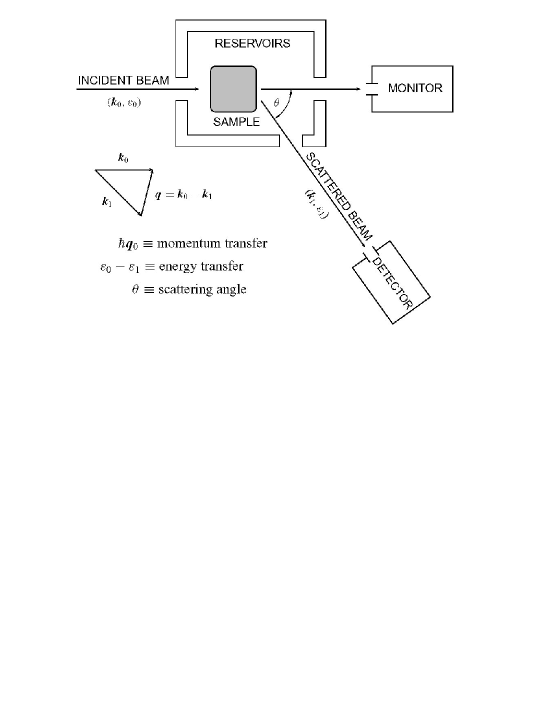
Figure 2: Scheme of an experiment of scattering.

Calling $\epsilon_{1}$ and $\hbar\mathbf{k}_{1}$ the energy and momentum of the scattered particle, conservation of energy and momentum require that

$$\Delta E=\varepsilon_{0}-\varepsilon_{1}\;,$$ (111)

$$\hbar\mathbf{q}=\hbar\mathbf{k}_{0}-\hbar\mathbf{k}_{1}\;,$$ (112)

or

$$q^{2}=k_{0}^{2}+k_{1}^{2}-2k_{0}k_{1}\cos\theta$$ (113)

after scalar product of Eq. (112) with itself ($\theta$ is the so-called scattering angle, see Fig. 2).

Let us go over the general theory: The scattering can be characterized by the quantity differential scattering cross section, $d^{2}\sigma(\Delta E,\mathbf{q})$. It is defined as the ratio between the number of scattered particles that are collected by a detector within an element of solid angle $d\Omega(\theta,\varphi)$ in direction $(\theta,\varphi)$ per unit time (to be designated $\delta\dot{N}$), and the flux of incident particles, namely the number of particles that enter the sample per unit of time and unit of area (to be designated $\Phi_{0}$). The latter is given by

$$\Phi_{0}=nv_{0}\;,$$ (114)

where $n$ is the density of incident particles and $v_{0}$ their mean velocity (e.g. velocity of light in the case of photons, the thermal velocity in the case of thermalized neutrons). On the other hand we have that

$$\delta\dot{N}=nV\sum_{\mathbf{p}_{1}^{\prime}\in d\Omega}w_{\mathbf{p}_{0}\rightarrow\mathbf{p}_{1}^{\prime}}(\Delta E)\;,$$ (115)

where $w$ is the probability per unit time that an incident particle with momentum $\mathbf{p}_{0}$ makes a transition to a state of momentum $\mathbf{p}_{1}^{\prime}$, the latter in directions contained in the solid angle $d\Omega(\theta,\varphi)$ whose axis we indicate by $\mathbf{p}_{1}$ (or $\hbar\mathbf{k}_{1}$); $\Delta E$ is the transfer of energy in the scattering event, and $nV$ is the number of particles and $V$ is the active volume of the sample, i.e. the region involved in the process, for example the region of focalization of the laser beam in the scattering of photons.

However, since $d\Omega$ is small (fixed by the size of the detector window) we can take all the contributions in the sum over $\mathbf{p}_{1}$ as the same, i.e. to a good degree of approximation equal to $w_{\mathbf{p}_{0}\rightarrow\mathbf{p}_{1}}(\Delta E)$. Hence

$$d^{2}\sigma(\Delta E,\mathbf{q})=\frac{\delta\dot{N}}{\Phi_{0}}=\frac{V}{v_{0}}w_{\mathbf{p}_{0}\rightarrow\mathbf{p}_{1}}(\Delta E)b(\mathbf{p}_{1},d\Omega)\;,$$ (116)

where

$$b(\mathbf{p},d\Omega)=\sum_{\mathbf{p}_{1}^{\prime}\in d\Omega}1\simeq\frac{V}{(2\pi\hbar)^{3}}p_{1}^{2}dp_{1}d\Omega$$ (117)

is the number of states of the particles in the scattered beam, which are entering the detector, and we recall that $\mathbf{p}=\hbar\mathbf{k}$ and the sum is over the plane-wave state of wavevector $\mathbf{k}$.

Therefore, for calculating the differential cross section we need to evaluate the transition probability per unit time, $w$. For that purpose let us consider a system with Hamiltonian $\hat{H}_{\sigma}$, let us call $\hat{H}_{P}$ the Hamiltonian of the particles used in the experiment, and $\hat{\mathcal{V}}$ the interaction potential between the system and the particles, that is

$$\hat{H}=\hat{H}_{\sigma}+\hat{H}_{P}+\hat{\mathcal{V}}\;.$$ (118)

Let us introduce the notation $|\mu\rangle$ and $|\mathbf{p}\rangle$ for the eigenfunctions of the system and the particles in the probe, i.e.

$$\hat{H}_{\sigma}|\mu\rangle=E_{\mu}|\mu\rangle\;,$$ (119)

$$\hat{H}_{P}|\mathbf{p}\rangle=\hbar\omega_{\mathbf{p}}|\mathbf{p}\rangle\;,$$ (120)

where states $|\mathbf{p}\rangle$ are plane waves for the free particle with momentum $\mathbf{p}$ in the incident and scattered beams. Moreover, let

$$|\psi(t_{i})\rangle=|\Phi(t_{i})\rangle|\mathbf{p}_{0}(t_{i})\rangle$$ (121)

be the wavefunction at the initial time $t_{i}$, that is, the initial preparation of the system in the experiment.

As we have seen in previous sections, it is convenient to work in the interaction representation, and then the wavefunction of the system and probe at time $t$ is

$$|\psi(t)\rangle=U_{0}(t,t_{i})U^{\prime}(t,t_{i})|\psi(t_{i})\rangle$$ (122)

[cf. Eqs. (5) to (8)], with

$$i\hbar\frac{\partial}{\partial t}U^{\prime}(t,t_{i})=\tilde{\mathcal{V}}(t)U^{\prime}(t,t_{i})\;,$$ (123)

where $\tilde{\mathcal{V}}(t)$ is the potential in the interaction representation, i.e. evolving with $\hat{H}_{0}=\hat{H}_{\sigma}+\hat{H}_{p}$, [cf. Eqs. (9) and (10)], $U_{0}$ is given by

$$U_{0}(t,t_{i}) = U_{\sigma}(t,t_{i})U_{P}(t,t_{i})$$ (124)

$$= e^{\frac{1}{i\hbar}(t-t_{i})\hat{H}_{\sigma}}e^{\frac{1}{i\hbar}(t-t_{i})\hat{H}_{P}}\;,$$

and we recall that the iterated solution of Eq. (10) is given in Eq. (11).

Moreover, if we define the function

$$|\tilde{\psi}(t)\rangle=U_{0}^{\dagger}(t,t_{i})|\psi(t)\rangle=U^{\prime}(t,t_{i})|\psi(t_{i})\rangle\;,$$ (125)

we can easily verify that it satisfies the equation

$$i\hbar\frac{\partial}{\partial t}|\tilde{\psi}(t)\rangle=\tilde{\mathcal{V}}(t)|\tilde{\psi}(t)\rangle\;,$$ (126)

with $|\tilde{\psi}(t_{i})\rangle=|\psi(t_{i})\rangle$, which can be rewritten as

$$|\tilde{\psi}(t)\rangle=|\psi(t_{i})\rangle+\frac{1}{i\hbar}\int_{t_{i}}^{t}dt^{\prime}\,\tilde{\mathcal{V}}(t^{\prime})|\tilde{\psi}(t^{\prime})\rangle\;,$$ (127)

and then has the iterated solution

$$|\tilde{\psi}(t)\rangle=\Biggl{[}\,\sum_{n=0}^{\infty}\frac{1}{(i\hbar)^{n}}\int_{t_{i}}^{t}dt_{1}\cdots\int_{t_{i}}^{t_{n-1}}dt_{n}\,\tilde{\mathcal{V}}(t_{1})\cdots\tilde{\mathcal{V}}(t_{n})\Biggr{]}|\psi(t_{i})\rangle\;,$$ (128)

and for later convenience in the calculations we notice that we can write that

$$\tilde{\mathcal{V}}(t)|\tilde{\psi}(t)\rangle=\tilde{\varXi}(t)|\psi(t_{i})\rangle\;,$$ (129)

with $\tilde{\varXi}$, called the scattering operator, satisfying the integral equation

$$\tilde{\varXi}(t)=\tilde{\mathcal{V}}(t)\Biggl{[}1+\frac{1}{i\hbar}\int_{t_{i}}^{t}dt^{\prime}\,\tilde{\varXi}(t^{\prime})\Biggr{]}\;.$$ (130)

It can be noticed that the right hand side of Eq. (128) provides the effect of the perturbation $\mathcal{V}$ in all orders over the initial nonperturbed wavefunction, equivalent to the effect in first order over the interaction-representation function $|\tilde{\psi}(t)\rangle$.

Let us now fix the scattering channel, i.e. we consider, as required by Eq. (115), the scattering event with probe particles making transitions between states of momentum $|\mathbf{p}_{0}\rangle$ and $|\mathbf{p}_{1}\rangle$. According to the general theory of Quantum Mechanics, the probability for this event at time $t$ is given by

$$P_{\mathbf{p}_{0}\rightarrow\mathbf{p}_{1}}(t)=\sum_{\mu}|\langle\mathbf{p}_{1},\mu|\psi(t)\rangle|^{2}\;,$$ (131)

where the summation over all states $|\mu\rangle$ of the system will be a posteriori restricted by the selection rule involving conservation of energy and momentum in the scattering events.

We can rewrite Eq. (131) as

$$P_{\mathbf{p}_{0}\rightarrow\mathbf{p}_{1}}(t) = \sum_{\mu}|\langle\mathbf{p}_{1},\mu|U_{0}(t,t_{i})U^{\prime}(t,t_{i})|\psi(t_{i})\rangle|^{2}$$ (132)

$$= \sum_{\mu}|\langle\mathbf{p}_{1},\mu|U_{0}(t,t_{i})|\tilde{\psi}(t)\rangle|^{2}\;,$$

where we have used Eq. (125). On the other hand

$$\langle\mathbf{p},\mu|U_{0}(t,t_{i})=\langle\mathbf{p},\mu|\exp\Biggl{\{}-\frac{1}{i\hbar}(t-t_{i})(E_{\mu}+\hbar\omega_{\mathbf{p}})\Biggr{\}}\;,$$ (133)

then the exponential gives a modulus 1 in Eq. (132), and we have that

$$P_{\mathbf{p}_{0}\rightarrow\mathbf{p}}(t) = \sum_{\mu}|\langle\mathbf{p}_{1},\mu|\psi(t)\rangle|^{2}$$ (134)

$$= \sum_{\mu}|\langle\mathbf{p}_{1},\mu|[1+\frac{1}{i\hbar}\int_{t_{i}}^{t}dt^{\prime}\,\tilde{\varXi}(t^{\prime})]|\psi(t_{i})\rangle|^{2}$$

$$= \sum_{\mu}|\langle\mathbf{p}_{1},\mu|\frac{1}{i\hbar}\int_{t_{i}}^{t}dt^{\prime}\tilde{\varXi}(t^{\prime})|\Phi(t_{i}),\mathbf{p}_{0}\rangle|^{2}\;,$$

where we have used Eqs. (127) and (129), together with Eq. (121), and the fact that the plane wave states $|\mathbf{p}_{0}\rangle$ and $|\mathbf{p}_{1}\rangle$ are orthonormal states.

Introducing

$$\tilde{\varXi}_{\mathbf{q}}(t)=\langle\mathbf{p}_{1}|\tilde{\varXi}(t)|\mathbf{p}_{0}\rangle=\int d^{3}r\,\frac{e^{\frac{1}{i\hbar}\mathbf{p}_{1}\cdot\mathbf{r}}}{\sqrt{V}}\tilde{\varXi}(t)\frac{e^{-\frac{1}{i\hbar}\mathbf{p}_{0}\cdot\mathbf{r}}}{\sqrt{V}}\;,$$ (135)

with, we recall, $\hbar\mathbf{q}=\mathbf{p}_{0}-\mathbf{p}_{1}$, and using that the squared modulus can be written as the product of the complex number times its complex conjugate, we can write

$$P_{\mathbf{p}_{0}\rightarrow\mathbf{p}_{1}}(t) = \frac{1}{\hbar^{2}}\sum_{\mu}\langle\phi(t_{i})|\int_{-\infty}^{t}dt^{\prime\prime}\tilde{\varXi}_{\mathbf{q}}^{\dagger}(t^{\prime\prime})|\mu\rangle\langle\mu|\int_{-\infty}^{t}dt^{\prime}\,\tilde{\varXi}_{\mathbf{q}}(t^{\prime})|\Phi(t_{i})\rangle$$ (136)

$$= \frac{1}{\hbar^{2}}\int_{-\infty}^{t}dt^{\prime}\int_{-\infty}^{t}dt^{\prime\prime}Tr\bigl{\{}\tilde{\varXi}_{\mathbf{q}}^{\dagger}(t^{\prime\prime})\tilde{\varXi}_{\mathbf{q}}(t^{\prime})\mathcal{P}_{0}(t_{i})\bigr{\}}\;,$$

with $\mathcal{P}_{0}(t_{i})$ being the projection operator (statistical operator for the pure state $|\Phi(t_{i})\rangle$ of Eq. (121), and we have considered adiabatic application of the perturbation in $t_{i}\rightarrow-\infty$), implying in that the initial ultrafast transient is ignored.

So far we have a purely quantum-mechanical calculation, and we have an expression depending on the initial preparation of the system as characterized by the statistical operator for the pure state given above. We need next to introduce the statistical average over the mixed state, what is done averaging over the corresponding Gibbs ensemble of all possible initial pure states compatible with the thermodynamic condition of preparation of the system at time $t_{i}$, that is, we do have have that

$$\langle P_{\mathbf{p}_{0}\rightarrow\mathbf{p}_{1}}(t)\rangle=\frac{1}{\hbar^{2}}\int_{-\infty}^{t}dt^{\prime}\int_{-\infty}^{t}dt^{\prime\prime}Tr\bigl{\{}\tilde{\varXi}_{\mathbf{q}}^{\dagger}(t^{\prime\prime})\tilde{\varXi}_{\mathbf{q}}(t^{\prime})\varrho_{\varepsilon}(t_{i})\times\varrho_{R}\bigr{\}}$$ (137)

where $\varrho_{\varepsilon}(t_{i})\times\varrho_{R}=\mathcal{R}_{\varepsilon}(t_{i})$ is the corresponding statistical operator, involving $\varrho_{\varepsilon}$ of the system in interaction with the thermal bath and $\varrho_{R}$ of the thermal bath, which has been assumed to constantly remain in equilibrium at temperature $T_{0}$.

The rate of transition probability $w$ in Eq. (116), is then

$$w_{\mathbf{p}_{0}\rightarrow\mathbf{p}_{1}}(\Delta E|t) = \frac{d}{dt}\langle P_{\mathbf{p}_{0}\rightarrow\mathbf{p}_{1}}(t)\rangle$$ (138)

$$= \frac{1}{\hbar^{2}}\int_{-\infty}^{t}dt^{\prime}Tr\{\tilde{\varXi}_{\mathbf{q}}^{\dagger}(t)\tilde{\varXi}_{\mathbf{q}}(t^{\prime})\varrho_{\varepsilon}(t_{i})\times\varrho_{R}\}+$$

$$\frac{1}{\hbar^{2}}\int_{-\infty}^{t}dt^{\prime}Tr\{\tilde{\varXi}_{\mathbf{q}}^{\dagger}(t^{\prime})\tilde{\varXi}_{\mathbf{q}}(t)\varrho_{\varepsilon}(t_{i})\times\varrho_{R}\}\,\,.$$

Using that

$$Tr\{U_{0}^{\dagger}(t,t_{i})\tilde{\varXi}_{\mathbf{q}}^{\dagger}U(t,t_{i})U_{0}^{\dagger}(t^{\prime},t_{i})\tilde{\varXi}_{\mathbf{q}}U_{0}(t^{\prime},t_{i})\mathcal{R}_{\varepsilon}(t_{i})\}=Tr\{\tilde{\varXi}_{\mathbf{q}}^{\dagger}\tilde{\varXi}_{\mathbf{q}}(t^{\prime}-t)\varrho_{\varepsilon}(t)\times\varrho_{R}\}\;,$$ (139)

and that

$$\tilde{\varXi}_{\mathbf{q}}(t^{\prime}-t) = \langle\mathbf{p}_{1}|U_{P}^{\dagger}(t^{\prime}-t)U_{\sigma}^{\dagger}(t^{\prime}-t)\tilde{\varXi}_{\mathbf{q}}U_{\sigma}(t^{\prime}-t)U_{P}(t^{\prime}-t)|\mathbf{p}_{0}\rangle$$ (140)

$$= e^{-\frac{1}{i\hbar}(t^{\prime}-t)\hbar(\omega_{\mathbf{p}_{0}}-\omega_{\mathbf{p}_{1}})}\tilde{\varXi_{\mathbf{q}}}(t^{\prime}-t)_{\sigma}\;,$$

where $\tilde{\varXi}_{\mathbf{q}}(t^{\prime}-t)_{\sigma}=U_{\sigma}^{\dagger}(t^{\prime}-t,t_{i})\tilde{\varXi}_{\mathbf{q}}U_{\sigma}(t^{\prime}-t,t_{i})$, we can write

$$w_{\mathbf{p}_{0}\rightarrow\mathbf{p}_{1}}(\Delta E|t) \equiv w(\mathbf{q},\omega|t)$$ (141)

$$= \frac{1}{\hbar^{2}}\int_{-\infty}^{t}dt^{\prime}\,e^{i\omega(t^{\prime}-t)}Tr\{\tilde{\varXi}_{\mathbf{q}}^{\dagger}\tilde{\varXi}_{\mathbf{q}}(t^{\prime}-t)_{\sigma}\varrho_{\varepsilon}(t)\times\varrho_{R}\}+\text{ c.c.}\;,$$

where $\omega=\omega_{\mathbf{p}_{0}}-\omega_{\mathbf{p}_{1}}$, and it can be noticed that the statistical operator is given at time $t$, when a measurement is performed.

If we consider the case of equilibrium, i.e. we take the canonical distribution $\varrho_{c}$ instead of $\varrho_{\varepsilon}(t)$, and taking into account that $\varrho_{c}$ and $H_{\sigma}$ commute, we find that

$$w(\mathbf{q},\omega)_{\text{eq}}=\frac{1}{\hbar^{2}}\int_{-\infty}^{\infty}d\tau^{\prime}\,e^{-i\omega\tau^{\prime}}Tr\{\tilde{\varXi}_{\mathbf{q}}^{\dagger}(\tau^{\prime})_{\sigma}\tilde{\varXi}_{\mathbf{q}}\varrho_{c}\}\;,$$ (142)

which is the known temperature-dependent rate of transition probability (see for example [50]).

In conclusion, the differential cross section is then given by

$$\frac{d^{2}\sigma(\mathbf{q},\omega|t)}{d\omega\,d\Omega} = \frac{V^{2}}{(2\pi\hbar)^{3}}\frac{g(\omega)}{v_{0}}\frac{1}{\hbar^{2}}\Biggl{[}\int_{-\infty}^{t}dt^{\prime}\,e^{i\omega(t^{\prime}-t)}Tr\{\tilde{\varXi}_{\mathbf{q}}^{\dagger}\tilde{\varXi}_{\mathbf{q}}(t^{\prime}-t)_{\sigma}\mathcal{R}_{\varepsilon}(t)\}+$$ (143)

$$\int_{-\infty}^{t}dt^{\prime}\,e^{-i\omega(t^{\prime}-t)}Tr\{\tilde{\varXi}_{\mathbf{q}}^{\dagger}(t^{\prime}-t)_{\sigma}\tilde{\varXi}_{\mathbf{q}}\varrho_{\varepsilon}(t)\times\varrho_{R}\}\Biggr{]}\;,$$

each term within the square bracket is the complex conjugate of the other and then the quantity is real, as it should, and we have defined

$$p^{2}dp=g(\omega)\,d\omega\;,$$ (144)

introducing the density of states $g(\omega)$ which follows in each case once it is given the dispersion relation $\omega_{\mathbf{p}}$.

Moreover it is stressed the fact that, differently to the case when the system is in equilibrium, in the nonequilibrium initial preparation of the sample the scattering cross section is not closed in itself, but it needs to be coupled to the set of kinetic equations that describe the evolution of the out of equilibrium system, i.e., those that determine the statistical operator $\mathcal{R}_{\varepsilon}(t)$. It can be noticed that this is a question also present in the response function theory of the previous sections.

As it has been noticed in previous Section, we can write $\mathcal{R}_{\varepsilon}(t)=\varrho_{\varepsilon}(t)\times\varrho_{R}$ and make use of the separation $\varrho_{\varepsilon}(t)=\bar{\varrho}(t)+\varrho_{\varepsilon}^{\prime}(t)$ to obtain that

$$d^{2}\sigma(\mathbf{q},\omega|t)=d^{2}\bar{\sigma}(\mathbf{q},\omega|t)+d^{2}\bar{\sigma}_{\varepsilon}^{\prime}(\mathbf{q},\omega|t)\,,$$ (145)

that is, the contribution $d^{2}\bar{\sigma}$ where the trace is taken with $\bar{\varrho}$ and $d^{2}\sigma_{\varepsilon}^{\prime}$ with the trace taken with $\varrho_{\varepsilon}^{\prime}$.

Let us consider the case of time- and space- resolved scattering, that is the detector in Fig. 2 collects the scattered particles arriving from an element of volume $\Delta V(\mathbf{r})$ around position $\mathbf{r}$ in the sample. For simplicity we take the first-order scattering consisting that in Eq. (142) we take of the scattering operator $\Xi$ of Eq. (130) the first contribution $\mathcal{\bar{V}}$, and for the latter we write

$$\mathcal{\hat{V}}=\sum\limits_{\mu=1}^{N^{\prime}}\sum\limits_{j=1}^{N}\upsilon(\mathbf{R}_{\mu}-\mathbf{r}_{j})\,,$$ (146)

where $\mathbf{r}_{j}$ is the position of j-th particle in the system and $\mathbf{R}_{\mu}$ the position of the $\mu$-th particle in the incident beam.

Therefore, we have that

$$\mathcal{\hat{V}}_{\mathbf{q}}=\langle\mathbf{p}_{0}|\mathcal{\hat{V}}|\mathbf{p}_{1}\rangle=n_{b}\upsilon(\mathbf{q})\sum\limits_{j=1}^{N}e^{i\mathbf{q}\cdot\mathbf{r}_{j}}\,,$$ (147)

where we have introduced the Fourier amplitude

$$\upsilon(\mathbf{q})=\int d^{3}b\upsilon(b)e^{i\mathbf{q}\cdot\mathbf{b}}\,,$$ (148)

with $\mathbf{b}=\mathbf{r}-\mathbf{r}_{j}$, and we recall that $\hbar\mathbf{q}=\mathbf{p}_{0}-\mathbf{p}_{1}$, and $n_{b}$ is the density of particles in the beam.

Retaining in Eq. (143) the contribution in first order in $\mathcal{V}$ only, it follows that

$$\frac{d^{2}\sigma(\mathbf{q},\omega|t)}{d\omega d\Omega}=\frac{V^{2}}{(2\pi\hbar)^{3}}\frac{g(\omega)}{\hbar^{2}v_{0}}n_{b}^{2}|\upsilon(\mathbf{q})|^{2}S_{nn}(\mathbf{q},\omega|t)\,,$$ (149)

where

$$S_{nn}(\mathbf{q},\omega|t)=\sum\limits_{j,l}\int_{-\infty}^{t}dt^{\prime}\,e^{i\omega(t^{\prime}-t)}Tr\{e^{-i\mathbf{q}\cdot[\mathbf{r}_{j}(t^{\prime}-t)-\mathbf{r}_{l}]}\varrho_{\varepsilon}(t)\times\varrho_{R}\}+\text{c.c.}\;,$$ (150)

We introduce now the density operator

$$\hat{n}(\mathbf{r},\tau)=\sum\limits_{j}\delta(\mathbf{r}-\mathbf{r}_{j}(t))$$ (151)

and then we can rewrite the correlation function of Eq. (150) as

$$S_{nn}(\mathbf{q},\omega|t)=\int d^{3}r\int d^{3}r^{\prime}\int_{-\infty}^{t}dt^{\prime}\,e^{i\omega(t^{\prime}-t)}e^{-i\mathbf{q}\cdot(\mathbf{r}-\mathbf{r}^{\prime})}Tr\{\hat{n}^{{\dagger}}(\mathbf{r},t^{\prime}-t)\hat{n}(\mathbf{r}^{\prime})\varrho_{\varepsilon}(t)\times\varrho_{R}\}+\text{c.c.}\;,$$ (152)

where the integrations in space run over the active volume of the sample (region of concentration of the particle beam), or in the case of a space-resolved experiment over $\Delta V(\mathbf{r})$ and then we do have the time- and space- resolved spectrum

$$\frac{d^{2}\sigma(\mathbf{r};\mathbf{q},\omega|t)}{d\omega d\Omega}=\Delta V(\mathbf{r})\int d^{3}r^{\prime}\int_{-\infty}^{t}dt^{\prime}\,e^{i\omega(t^{\prime}-t)}e^{-i\mathbf{q}\cdot(\mathbf{r}-\mathbf{r}^{\prime})}Tr\{\hat{n}^{{\dagger}}(\mathbf{r},t^{\prime}-t)\hat{n}(\mathbf{r}^{\prime})\varrho_{\varepsilon}(t)\times\varrho_{R}\}+\text{c.c.}\,,$$ (153)

In the case of an experiment in photoluminescence (recombination of photoexcited electrons and holes) the potential has the form

$$\mathcal{V}=\sum\limits_{j}\mathbf{A}(\mathbf{r}_{j},t)\cdot\mathbf{p}_{j}\,,$$ (154)

and then, after neglecting the photon momentum (dipolar approximation), the luminescence spectrum is given by

$$P_{L}(\mathbf{r};\omega|t)\sim\sum\limits_{\mathbf{k}}\bar{f}_{\mathbf{k}}^{\,e}(\mathbf{r},t)\bar{f}_{\mathbf{k}}^{\,h}(\mathbf{r},t)\delta(\hbar k^{2}/2m_{x}+E_{G}-\hbar\omega)\,,$$ (155)

in arbitrary units, where we have introduced a local approximation and it has been used the effective mass approximation for electrons ($e$) and holes ($h$), $m_{x}^{-1}=m_{e}^{-1}+m_{h}^{-1}$ is the excitonic mass, $E_{G}$ is the energy gap, and $\bar{f}_{\mathbf{k}}^{\,e(h)}(\mathbf{r},t)$ are the populations in state $\mathbf{k}$, in position $\mathbf{r}$ and at time $t$ of electrons (holes) given by

$$\bar{f}_{\mathbf{k}}^{\,e(h)}(\mathbf{r},t)=[1+\exp\{\beta^{\ast}(\mathbf{r},t)[\hbar^{2}k^{2}/2m_{e(h)}-\mu_{e(h)}^{\ast}(\mathbf{r},t)]^{-1}\}\,,$$ (156)

where $\beta^{\ast}(\mathbf{r},t)$ is the reciprocal of the field of nonequilibrium temperature and $\mu_{e(h)}^{\ast}(\mathbf{r},t)$ the quasi-chemical potential.

VI Illustrative Examples

VI.1 Experiments in ultra-fast-laser spectroscopy.

Pump-probe experiments in the field of ultrafast laser spectroscopy, devoted to the study of the nonequilibrium photoinjected plasma in semiconductors, have been extensively used in recent decades, and have been accompanied by a number of theoretical analysis [58-64]. In this type of experiments the system is, as a general rule, driven far away from equilibrium and consequently, its theoretical description falls into the realm of the thermodynamics of irreversible processes in far-from-equilibrium systems, and the accompanying kinetic and statistical theories, and a particularly appropriate approach is the nesef described here. The theory presented in the previous Section has been used to derive in detail a response function theory for the study of ultrafast optical properties in the photoinjected plasma in semiconductors. Particularly, one needs to derive the frequency- and wave number-dependent dielectric function in arbitrary nonequilibrium conditions, because it is the quantity which contains all the information related to the optical properties of the system (it provides the absorption coefficient, the reflectivity coefficient, the Raman scattering cross section, and so on). This is described below, and moreover, we describe the application of the results to the study of a particular type of experiment, namely the time-resolved reflectivity changes in GaAs and other materials [51-54] where signal changes in the reflectivity, $\Delta R/R$, of the order of $10^{-7}$ are detected, and a distinct oscillation of the signal in real time is observed. In Fig. 3 are reproduced time-resolved reflectivity spectra, and in the upper right inset is shown the part corresponding to the observed oscillation, as reported by Cho et al. [51]

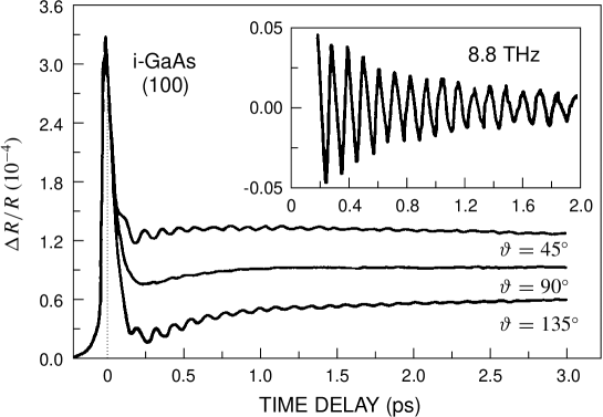
Figure 3: Reproduction of the time-resolved reflectivity changes in GaAs, as reported by Cho, Kütt, and Kurz in Ref. [51].

Such phenomenon has been attributed to the generation of coherent lattice vibrations, and several theoretical approaches have been reported [54-56]. A clear description, on phenomenological bases, which captures the essential physics of the problem, is reported in Ref. [55], and in Ref. [57] is presented an analysis based on nesef, where the different physical aspects of the problem are discussed. It is evidenced that the oscillatory effect is provided by the displacive excitation of the polar lattice vibrations, arising out of the coupling of the carrier-charge density and polar modes, and its decay is mainly governed by the cooling down of the carriers. We briefly describe the experiment and all the pertaining nesef-based calculations in continuation.

Let us consider a direct-gap polar semiconductor in a pump-probe experiment. We recall that the exciting intense laser pulse produces the so-called highly excited plasma in semiconductors, namely, electron-hole pairs in the metallic side of Mott transition (that is, they are itinerant carriers, and we recall that this requires concentrations of these photoinjected quasi-particles of order of $10^{16}$ cm^-3 and up), which compose a two-component Fermi fluid, moving in the lattice background. It constitutes a highly nonequilibrated system where the photoexcited carriers rapidly redistribute their energy in excess of equilibrium via, mainly, the strong long-range Coulomb interaction (pico- to subpico- second scale), followed by the transfer of energy to the phonon field (predominantly to the optical phonons, and preferentially to the lo phonons via Fröhlich interaction), and finally via acoustic phonons to the external thermal reservoir. Along the process the carrier density diminishes in recombination processes (nanosecond time scale) and through ambipolar diffusion out of the active volume of the sample (ten-fold picosecond time scale).

Moreover, a probe interacting weakly with the heps is used to obtain an optical response, namely the reflectivity of the incoming laser photons with frequency $\omega$ and wave vector $\mathbf{Q}$. From the theoretical point of view, such measurement is to be analyzed in terms of, as already noted, the all important and inevitable use of correlation functions in response function theory. The usual application in normal probe experiments performed on a system initially in equilibrium had a long history of success, and a practical and elegant treatment is based on the method of the double-time (equilibrium) thermodynamic Green functions [45,46]. In the present case of a pump-probe experiment we need to resort to a theory of such type but applied to a system whose macroscopic state is in nonequilibrium conditions and evolving in time as a result of the dissipative processes that are developing while the sample is probed. This is, resorting to the theory of previous section, and we recall that the response function theory for nonequilibrium systems needs be coupled to the kinetic theory that describes the evolution of the nonequilibrium state of the system. We resort here to such theory for the study of the reflectivity experiments of Ref. [51].

The time-dependent (because it keeps changing along with the evolution of the macrostate of the nonequilibrated system) reflectivity $R(\omega,\mathbf{Q}|t)$ is related to the index of refraction $\eta(\omega,\mathbf{Q}|t)+i\kappa(\omega,\mathbf{Q}|t)$ through the well-known expression

$$R(\omega,\mathbf{Q}|t)=\frac{\left[\eta(\omega,\mathbf{Q}|t)-1\right]^{2}+\left[\kappa(\omega,\mathbf{Q}|t)\right]^{2}}{\left[\eta(\omega,\mathbf{Q}|t)+1\right]^{2}+\left[\kappa(\omega,\mathbf{Q}|t)\right]^{2}}\;,$$ (157)

and the refraction index is related to the time-evolving frequency- and wave vector-dependent dielectric function by

$$\epsilon(\omega,\mathbf{Q}|t) = \epsilon^{\prime}(\omega,\mathbf{Q}|t)+i\epsilon^{\prime\prime}(\omega,\mathbf{Q}|t)$$ (158)

$$= \left[\eta(\omega,\mathbf{Q}|t)+i\kappa(\omega,\mathbf{Q}|t)\right]^{2}\;,$$

where $\eta$ and $\epsilon^{\prime}$, and $\kappa$ and $\epsilon^{\prime\prime}$, are the real and imaginary parts of the refraction index and of the dielectric function respectively.

We call the attention to the fact that the dielectric function depends on the frequency and the wave vector of the radiation involved, and $t$ stands for the time when a measurement is performed. Once again we stress that this dependence on time is, of course, the result that the macroscopic state of the non-equilibrated plasma is evolving in time as the experiment is performed.

Therefore it is our task to calculate this dielectric function in the nonequilibrium state of the system. First, we note that according to Maxwell equations in material media (that is, Maxwell equations now averaged over the nonequilibrium statistical ensemble) we have that

$$\epsilon^{-1}(\omega,\mathbf{Q}|t)-1=\frac{n(\omega,\mathbf{Q}|t)}{r(\omega,\mathbf{Q})}\;,$$ (159)

where $r(\omega,\mathbf{Q})$ is the amplitude of a probe charge density with frequency $\omega$ and wave vector $\mathbf{Q}$, and $n(\omega,\mathbf{Q}|t)$ is the induced polarization-charge density of carriers and lattice in the media. As shown before the latter can be calculated resorting to the response function theory for systems far from equilibrium (the case is quite similar to the calculation of the time-resolved Raman scattering cross section [48]), and obtained in terms of the nonequilibrium-thermodynamic Green functions, as we proceed to describe.

Using the formalism we have presented to obtain $\epsilon(\omega,\mathbf{Q}|t)$, [cf. Eqs. (98)] it follows that

$$\epsilon^{-1}(\omega,\mathbf{Q})-1=V(\mathbf{Q})\,[G_{cc}(\omega,\mathbf{Q})+G_{ci}(\omega,\mathbf{Q})+G_{ic}(\omega,\mathbf{Q})+G_{ii}(\omega,\mathbf{Q})]\;,$$ (160)

giving the reciprocal of the dielectric function in terms of Green functions given by

$$G_{cc}(\omega,\mathbf{Q})=\langle\!\langle\hat{n}_{c}(\mathbf{Q})\,;\,\hat{n}_{c}^{\dagger}(\mathbf{Q})|\,\omega;t\rangle\!\rangle\;,$$ (161)

$$G_{ci}(\omega,\mathbf{Q})=\langle\!\langle\hat{n}_{c}(\mathbf{Q})\,;\,\hat{n}_{i}^{\dagger}(\mathbf{Q})|\,\omega;t\rangle\!\rangle\;,$$ (162)

$$G_{ic}(\omega,\mathbf{Q})=\langle\!\langle\hat{n}_{i}(\mathbf{Q})\,;\,\hat{n}_{c}^{\dagger}(\mathbf{Q})|\,\omega;t\rangle\!\rangle\;,$$ (163)

$$G_{ii}(\omega,\mathbf{Q})=\langle\!\langle\hat{n}_{i}(\mathbf{Q})\,;\,\hat{n}_{i}^{\dagger}(\mathbf{Q})|\,\omega;t\rangle\!\rangle\;,$$ (164)

where $V(\mathbf{Q})=4\pi ne^{2}/V\varepsilon_{0}Q^{2}$ is the matrix element of the Coulomb potential in plane-wave states and $\hat{n}_{c}(\mathbf{Q})$, and $\hat{n}_{i}(\mathbf{Q})$, refer to the $\mathbf{Q}$-wave vector Fourier transform of the operators for the densities of charge of carriers and the polarization charge of longitudinal optical phonons respectively.

But, the expression we obtain is, as already noticed, depending on the evolving nonequilibrium macroscopic state of the system, a fact embedded in the expressions for the time-dependent distribution functions of the carrier and phonon states. Therefore, they are to be derived within the kinetic theory in nesef, and the first and fundamental step is the choice of the set of variables deemed appropriate for the description of the macroscopic state of the system. In this case a first set of variables needs be the one composed of the carriers’ density and energy, and the phonon population functions, together with the set of associated Lagrange multipliers that, as we have seen, can be interpreted as a reciprocal quasitemperature and quasi-chemical potentials of carriers, and reciprocal quasitemperatures of phonons, one for each mode [42,58,59]. But in the situation we are considering we need to add, on the basis of the information provided by the experiment, the amplitudes of the lo-lattice vibrations and the carrier charge density; the former because it is clearly present in the experimental data (the oscillation in the reflectivity) and the latter because of the lo-phonon-plasma coupling clearly present in Raman scattering experiments [60,61]). Consequently the chosen basic set of dynamical quantities is

$$\{\hat{H}_{c},\hat{N}_{e},\hat{N}_{h},\hat{n}_{\mathbf{kp}}^{e},\hat{n}_{\mathbf{kp}}^{h},\hat{\nu}_{\mathbf{q}},a_{\mathbf{q}},a_{\mathbf{q}}^{\dagger},H_{B}\}\;,$$ (165)

where

$$\hat{H}_{c}=\sum_{\mathbf{k}}\left[\varepsilon_{\mathbf{k}}^{e}\,c_{\mathbf{k}}^{\dagger}\,c_{\mathbf{k}}+\varepsilon_{\mathbf{k}}^{h}\,h_{-\mathbf{k}}^{\dagger}\,h_{-\mathbf{k}}\right]\;,$$ (166)

$$\hat{\nu}_{\mathbf{q}}=a_{\mathbf{q}}^{\dagger}\,a_{\mathbf{q}}\;,$$ (167)

$$\hat{N}_{e}=\sum_{\mathbf{k}}c_{\mathbf{k}}^{\dagger}c_{\mathbf{k}}\,\,,\qquad\hat{N}_{h}=\sum_{\mathbf{k}}h_{-\mathbf{k}}^{\dagger}\,h_{-\mathbf{k}}\,\,,$$ (168)

$$\hat{n}_{\mathbf{kp}}^{e}=c_{\mathbf{k}+\mathbf{p}}^{\dagger}c_{\mathbf{k}}\,\,,\qquad\hat{n}_{\mathbf{kp}}^{h}=h_{-\mathbf{k}-\mathbf{p}}h_{-\mathbf{k}}^{\dagger}\,\,,$$ (169)

with $c$ ($c^{\dagger}$), $h$ ($h^{\dagger}$), and $a$ ($a^{\dagger}$) being as usual annihilation (creation) operators in electron, hole, and lo-phonon states respectively ($\mathbf{k},\mathbf{p},\mathbf{q}$ run over the Brillouin zone). Moreover, the effective mass approximation is used and Coulomb interaction is dealt with in the random phase approximation, and then $\epsilon_{\mathbf{k}}^{e}=E_{G}+\hbar^{2}|\mathbf{k}|^{2}/2m_{e}$ and $\epsilon_{\mathbf{k}}^{h}=\hbar^{2}|\mathbf{k}|^{2}/2m_{h}$. Finally $H_{B}$ is the Hamiltonian of the lattice vibrations different from the lo one. We write for the nesef-nonequilibrium thermodynamic variables associated to the quantities of Eq. (165)

$$\{\beta_{c}(t),\;-\beta_{c}(t)\mu_{e}^{\ast}(t),\;-\beta_{c}(t)\mu_{h}^{\ast}(t),\;F_{\mathbf{kp}}^{e}(t),\;\\ F_{\mathbf{kp}}^{h}(t),\;\hbar\omega_{\mathbf{q}}\beta_{\mathbf{q}}(t),\;\varphi_{\mathbf{q}}(t),\varphi_{\mathbf{q}}^{\ast}(t),\;\beta_{0}\}\;,$$ (170)

respectively, where $\mu_{e}^{\ast}$ and $\mu_{h}^{\ast}$ are the quasi-chemical potentials for electrons and for holes; we write $\beta_{c}(t)=1/k_{B}T_{c}^{\ast}(t)$ introducing the carriers’ quasitemperature $T_{c}^{\ast}$; $\beta_{\mathbf{q}}(t)=1/k_{B}T_{\mathbf{q}}^{\ast}(t)$ introducing the lo-phonon quasitemperature per mode ($\omega_{\mathbf{q}}$ is the dispersion relation), $\beta_{0}=1\,/\,k_{B}\,T_{0}$ with $T_{0}$ being the temperature of the thermal reservoir. We indicate the corresponding macrovariables, that is, those which define the nonequilibrium thermodynamic Gibbs space as

$$\{E_{c}(t),\;n(t),\;n(t),\;n_{\mathbf{kp}}^{e}(t),\;n_{\mathbf{kp}}^{h}(t),\nu_{\mathbf{q}}(t),\;\langle a_{{}_{\mathbf{q}}}|t\rangle,\;\langle a_{\mathbf{q}}^{\dagger}|t\rangle=\langle a_{\mathbf{q}}|t\rangle^{\ast},\;E_{B}\}\;,$$ (171)

which are the statistical average of the quantities of Eq. (165), that is

$$E_{c}(t)=Tr\bigl{\{}\hat{H}_{c}\,\varrho_{\epsilon}(t)\times\varrho_{R}\bigr{\}}\;,$$ (172)

$$n(t)=Tr\bigl{\{}\hat{N}_{e(h)}\,\varrho_{\epsilon}(t)\times\varrho_{R}\bigr{\}}\;,$$ (173)

and so on, where $\varrho_{R}$ is the stationary statistical distribution of the reservoir and $n(t)$ is the carrier density, which is equal for electrons and for holes since they are produced in pairs in the intrinsic semiconductor. The volume of the active region of the sample (where the laser beam is focused) is taken equal to $1$ for simplicity.

Next step is to derive the equation of evolution for the basic variables that characterize the nonequilibrium macroscopic state of the system, and from them the evolution of the nonequilibrium thermodynamic variables. This is done according to the generalized nesef-based nonlinear quantum transport theory already described, but in the second-order approximation in relaxation theory. This is an approximation which retains only two-body collisions but with memory being neglected, consisting in the Markovian limit of the theory. It is sometimes referred to as the quasi-linear approximation in relaxation theory [43,44], a name we avoid because of the misleading word linear which refers to the lowest order in dissipation, however the equations are highly nonlinear.

The nesef-auxiliary (“instantaneously frozen”) statistical operator is in the present case given, in terms of the variables of Eq. (165) and the nonequilibrium thermodynamic variables of Eq. (171), by

$$\bar{\varrho}(t,0) = \exp\Bigl{\{}-\phi(t)-\beta_{c}^{\ast}(t)[\hat{H}_{c}-\mu_{e}^{\ast}(t)\,\hat{N}_{e}-\mu_{h}^{\ast}(t)\,\hat{N}_{h}]-$$ (174)

$$\sum_{\mathbf{kp}}[F_{\mathbf{kp}}^{e}(t)\,\hat{n}_{\mathbf{kp}}^{e}(t)+F_{\mathbf{kp}}^{h}(t)\,\hat{n}_{\mathbf{kp}}^{h}(t)]-$$

$$\sum_{\mathbf{q}}[\beta_{\mathbf{q}}^{\ast}(t)\,\hbar\,\omega_{\mathbf{q}}\,\hat{\nu}_{\mathbf{q}}+\varphi_{\mathbf{q}}(t)\,a_{\mathbf{q}}+\varphi_{\mathbf{q}}^{\ast}(t)\,a_{\mathbf{q}}^{\dagger}]-\beta_{0}\,H_{B}\Bigr{\}}\;,$$

where $\phi(t)$ ensures the normalization of $\bar{\varrho}(t,0)$.

Using such statistical operator the Green functions that define the dielectric function [cf. Eq. (160)] can be calculated. This is an arduous task, and in the process it is necessary to evaluate the occupation functions

$$f_{\mathbf{k}}(t)=Tr\{c_{\mathbf{k}}c_{\mathbf{k}}\varrho_{\varepsilon}(t)\}\;,$$ (175)

which is dependent on the variables of Eq. (171). The (nonequilibrium) carrier quasitemperature $T_{c}^{\ast}$ is obtained, and its evolution in time shown in Fig. 4.

Figure 4: Evolution of the carrier’s quasitemperature, calculated in the conditions of the experiment in the caption to Fig. 3.

Finally, in Fig. 5, leaving only as an adjustable parameter the amplitude – which is fixed fitting the first maximum –, is shown the calculated modulation effect which is compared with the experimental result (we have only placed the positions of maximum and minimum amplitude taken from the experimental data, which are indicated by the full squares).

Figure 5: The theoretically evaluated modulation of the time-resolved reflectivity in the conditions of Ref. [51], compared with the experimental data. For simplicity we have drawn only the positions of the maxima and minima of the figure in the inset of Fig. 3.

This demonstrates the reason of the presence of the observed modulating phenomenon in the reflectivity spectra, occurring with the frequency of the near zone center lo-phonon (more precisely the one of the upper $L_{+}$ hybrid mode [61]) with wave vector $\mathbf{Q}$, the one of the photon in the laser radiation field. The amplitude of the modulation is determined by the amplitude of the laser-radiation-driven carrier charge density which is coupled to the optical vibration, and then an open parameter in the theory to be fixed by the experimental observation. This study has provided, as shown, a good illustration of the full use of the formalism of nesef, with an application to a quite interesting experiment and where, we recall, the observed signal associated to the modulation is seven orders of magnitude smaller than the main signal on which is superimposed.

VI.2 Charge Transport in Doped Semiconductors

NESEF is particularly appropriate do describe the transient and steady state of semiconductors in the presence of intermediate to strong electric fields (say tens to hundreds of kV/cm), fields which drive the system far-from equilibrium. The question has large technological interest because of the presence of such situation in the integrated circuits of electronic and optoelectronic devices.

Let us consider a n-doped direct-gap polar semiconductor, in condition such that the extra electrons act as mobile carriers in the conduction band. We use the effective-mass approximation, and therefore parabolic band; this implies that in explicit applications it needs be controlled the fact that there exists an upper limiting value for the electric field strength, such that below this limit we are working with field intensities for which intervalley scattering can be neglected. The Hamiltonian of the system is

$$\hat{H}=\hat{H}_{0}+\hat{H}_{1}+\hat{H}_{AN}+\hat{H}_{CF}+\hat{W}\,,$$ (176)

where

$$\hat{H}_{0}=\sum\limits_{\mathbf{k}}(\hbar^{2}k^{2}/2m_{e}^{\ast})c_{\mathbf{k}}^{\dagger}c_{\mathbf{k}}\text{ }+\sum\limits_{\mathbf{q},\gamma}\hbar\omega_{\mathbf{q},\gamma}(b_{\mathbf{q}_{\gamma}}^{\dagger}b_{\mathbf{q}_{\gamma}}+1/2)\,,$$ (177)

is the Hamiltonian of free electrons and phonons in branches $\gamma=$ lo,ac, and

$$\hat{H}_{1}=\sum\limits_{\mathbf{k},\mathbf{q},\gamma,\sigma}[M_{\gamma}^{\sigma}(\mathbf{q})b_{\mathbf{q}_{\gamma}}c_{\mathbf{k}+\mathbf{q}_{\gamma}}^{\dagger}c_{\mathbf{k}}+M_{\gamma}^{\sigma\ast}(\mathbf{q})b_{\mathbf{q}_{\gamma}}^{\dagger}c_{\mathbf{k}}^{\dagger}c_{\mathbf{k}+\mathbf{q}_{\gamma}}\,]\,,$$ (178)

is the interaction Hamiltonian between them. In these equations $c(c^{\dagger})$ and $b(b^{\dagger})$ are annihilation (creation) operators in electron states $|\mathbf{k}>$, and of phonons in mode $|\mathbf{q}_{\gamma}>$ and branches $\gamma=$lo,ac (for longitudinal optical and acoustical ones respectively; to-phonons are ignored once they do not interact with the electrons in the conduction band). Quantity M~(q) is the matrix element of the interaction between carriers and $\gamma$-type phonons, with superscript $\sigma$ indicating the kind of interaction (polar, deformation potential, piezoelectric). Moreover, $\hat{H}_{AN}$ stands for the anharmonic interaction in the phonon system, and

$$\hat{H}_{CF}=-\sum\limits_{i}e\mathbf{E}\cdot\mathbf{r}_{i},$$ (179)

is the interaction of the electrons (with charge $-e$ and positions $\mathbf{r}_{i}$) with an electric field $\mathbf{F}$ of intensity $\mathcal{E}$. The interaction of the system with an external reservoir is taken care of by $\hat{W}$ in Eq. (35); the reservoir is taken as an ideal one – what is satisfactory in most cases – and then has its macroscopic (thermodynamic) state characterized by a canonical statistical distribution with temperature $T_{0}$.

Consider now the nonequilibrium thermodynamic state of the system: the presence of the electric field changes the energy of the electrons (they acquire energy in excess of equilibrium), and these carriers keep transferring this excess to the lattice and from the lattice to the thermal reservoir, and an electrical current (flux of electrons) follows. Thus, we need to choose as basic variables

$$\bigl{\{}E_{e}(t),N_{e}(t),\mathbf{P}_{e}(t),E_{LO}(t),E_{AC}(t),E_{R}\bigr{\}},$$ (180)

that is, respectively, the energy, number, and linear momentum of the carriers, the energies of the lo and ac phonons, and the energy of the reservoir; the latter is constant in time for being considered as an ideal one. The corresponding dynamical quantities are

$$\bigl{\{}\hat{H}_{e},\hat{N}_{e},\mathbf{\hat{P}}_{e},\hat{H}_{LO},\hat{H}_{AC},\hat{H}_{R}\bigr{\}},$$ (181)

i.e. the Hermitian operators for the partial Hamiltonians, the electron number and the linear momentum. We noticed that the above choice implies in disregarding electro-thermal effects, whose inclusion would require to introduce the flux of energy (heat current) of the carriers; it has a minor influence on the results to be reported.

According to the nonequilibrium statistical ensemble formalism described in section 2 of the preceding article, the nonequilibrium thermodynamic state of the system, in an alternative description to the one provided by the variables of Eq. (181), can be completely characterized by a set of intensive nonequilibrium thermodynamic variables (Lagrange multipliers that the variational construction of the formalism provides), namely

$$\bigl{\{}F_{e}(t),F_{ne}(t),\mathbf{F}_{e}(t),F_{LO}(t),F_{AC}(t),\beta_{0}\}\bigr{\}},$$ (182)

The variables in this Eq. (182) are present in the auxiliary statistical operator which the formalism introduces, in this case given by

$$\bar{\varrho}(t,0) = \exp\bigl{\{}-\phi(t)-F_{ne}(t)\hat{N}_{e}-F_{e}(t)\hat{H}_{e}-$$ (183)

$$-\mathbf{F}_{e}(t)\cdot\mathbf{\hat{P}}_{e}-F_{LO}(t)\hat{H}_{LO}-F_{AC}(t)\hat{H}_{AC}]\times\varrho_{R}\bigr{\}},$$

where $\varrho_{R}$ is the canonical distribution of the reservoir at temperature $T_{0}$. We recall that the operator of Eq. (183) is not the statistical operator describing the macroscopic state of the system, which is a superoperator of this one, and $\phi(t)$ (playing the role of a logarithm of a nonequilibrium partition function) ensures the normalization of $\bar{\varrho}(t,0)$ (see Appendix A).

The intensive nonequilibrium thermodynamic variables of Eq. (182) are usually redefined as

$$F_{e}(t)=\beta_{e}^{\ast}(t)=[k_{B}T_{e}^{\ast}(t)]^{-1},$$ (184)

$$F_{ne}(t)=-\beta_{e}^{\ast}(t)\mu_{e}^{\ast}(t),$$ (185)

$$\mathbf{F}_{e}(t)=-\beta_{e}(t)\mathbf{v}_{e}(t),$$ (186)

$$F_{LO}(t)=\beta_{LO}^{\ast}(t)=[k_{B}T_{LO}^{\ast}(t)]^{-1},$$ (187)

$$F_{AC}(t)=\beta_{AC}^{\ast}(t)=[k_{B}T_{AC}^{\ast}(t)]^{-1},$$ (188)

and we recall that $\beta_{0}$ [in Eq. (182)] is $[k_{B}T_{0}]^{-1}$. These Eqs. (184) to (188) introduce the so-called quasitemperatures, $T_{e}^{\ast}(t)$, $T_{LO}^{\ast}(t)$, $T_{AC}^{\ast}(t)$, of electrons and phonons, and the quasi-chemical potential $\mu_{e}^{\ast}(t)$ and the drift velocity $\mathbf{v}_{e}(t)$ of the electrons; $k_{B}$ is as usual Boltzmann constant.

Proceeding with the calculations of the equations of evolution of the basic variables, the corresponding set of equations of evolution are obtained, which have expressions of the form [42,59,62]

$$\frac{d}{dt}E_{e}(t)=-\frac{e}{m_{e}^{\ast}}\mathbf{E}\cdot\mathbf{P}_{e}(t)-J_{E_{e}}^{(2)}(t)\,\,,$$ (189)

$$\frac{d}{dt}\mathbf{P}_{e}(t)=-nVe\mathbf{E}+\mathbf{J}_{\mathbf{P}_{e}}^{(2)}(t)+\mathbf{J}_{\mathbf{P}_{e},imp}^{(2)}(t)\,\,,$$ (190)

$$\frac{d}{dt}E_{LO}(t)=J_{E_{LO}}^{(2)}(t)-J_{LO,AN}^{(2)}(t)\,\,,$$ (191)

$$\frac{d}{dt}E_{AC}(t)=J_{E_{AC}}^{(2)}(t)+J_{LO,AN}^{(2)}(t)-J_{AC,dif}^{(2)}(t)\,\,,$$ (192)

where, we recall, $E_{e}(t)$ is the carriers’ energy and $\mathbf{P}_{e}(t)$ the linear momentum; $E_{LO}(t)$ the energy of the lo phonons which strongly interact with the carriers via Fröhlich potential in these strong-polar semiconductors (hence it predominates over the nonpolar-deformation potential interaction and then the latter is disregarded); $E_{AC}(t)$ is the energy of the acoustic phonons playing the role of a thermal bath; and $\mathbf{E}$ stands for the constant electric field.

Let us analyze these equations term by term. In Eq. (189) the first term on the right accounts for the rate of energy transferred from the electric field to the carriers, and the second term accounts for the transfer of the resulting excess energy of the carriers to the phonons. In Eq. (190) the first term on the right is the driving force generated by the presence of the electric field. The second term is the rate of momentum transfer due to the interaction with the phonons, and the last one is a result of scattering by impurities (these two terms are then momentum relaxation contributions). In Eq. (191) and Eq. (192) the first term on the right describes the rate of change of the energy of the phonons due to interaction with electrons. More precisely they account for the gain of the energy transferred to them from the hot carriers and then the sum of contributions $J_{E_{LO}}^{(2)}(t)$ and $J_{E_{AC}}^{(2)}(t)$ is equal to the last in Eq. (189), but accompanied with a change of sign. The second term in Eq. (191) accounts for the rate of transfer of energy from the optical phonons to the acoustic ones, via anharmonic interaction. The contribution $J_{LO,AN}^{(2)}(t)$ is the same but with different sign in Eq. (191) and Eq. (192). Finally, the diffusion of heat from the ac phonons to the reservoir is accounted for in the last term in Eq. (192). The detailed expression for the collision operators are given in Ref. [42] (quantities $J$ are positive).

The solution of these equations allows for a detailed analysis of the nonequilibrium thermodynamic state and transport properties of these materials. Let us consider first the III-Nitride compounds, which nowadays present a particular interest as a result of their potential use in lasers and diodes emitting in the blue and ultraviolet region (see for example [63]).

Let us consider the steady state which follows very rapidly (in a hundred-fold femtosecond time scale), what can be understood on the basis of the action of the intense Fröhlich interaction in these strong polar semiconductors, with the rate of transfer of energy from carriers to lo phonons rapidly equalizing the rate of energy pumping from the external field of intensity $\mathcal{E}$, even at high fields. It is then characterized by the constant-in-time variables quasitemperature, $T_{e}^{\ast}$, drift velocity, $\mathbf{v}_{e}$, and quasi-chemical potential, $\mu_{e}^{\ast}$, all referring to the electron system, and $T_{LO}^{\ast}$, the quasitemperature of the lo phonons, and ta, the quasitemperature of the acoustic phonons. In Fig. 6 it is shown the dependence of $T_{e}^{\ast}$ with the electric field, while in Fig. 7 is presented such dependence for the drift velocity for n-doped GaN, with $n=$ 10¹⁷cm^-3. The quasi-chemical potential is determined by the values of the concentration and the electron quasitemperature, and the deviation of $T_{LO}^{\ast}$ and $T_{A}$ from the value in equilibrium is small and can be neglected.

Figure 6: Dependence of the quasitemperature $T_{e}^{\ast}$ with the electric field in the steady state of n-doped GaN. We have used $m^{\ast}=0.19m_{0}$, $\varepsilon_{0}=9.5$, a carrier concentration $n=$ 10¹⁷cm^-3, and the thermal bath temperature is $T_{0}=300$ K. After Ref. [64]

We can now proceed to calculate the cross section for scattering of light by electrons in the electric field $\mathcal{E}$. Taking into account that the interaction of electrons and radiation is given by

$$V_{ER}\mathbf{Q}=G(\mathbf{Q})\hat{n}_{\mathbf{Q}}+H.c.\,,$$ (193)

where $\hbar\mathbf{Q}$ is the momentum of the photon, $G(\mathbf{Q})$ is the matrix element of the interaction, and

$$\hat{n}_{\mathbf{Q}}=\sum\limits_{\mathbf{k}}\hat{n}_{\mathbf{kQ}}=\sum\limits_{\mathbf{k}}c_{\mathbf{k+Q}}^{{\dagger}}c_{\mathbf{k}}\,,$$ (194)

the cross section of Eq. (143), in first order in the scattering operator, is given by

$$\frac{d^{2}\sigma(\mathbf{Q},\omega)}{d\omega d\Omega}=\frac{V^{2}}{(2\pi\hbar)^{3}}\frac{\hbar\omega^{2}}{c^{4}}|G(\mathbf{Q})|^{2}\int\limits_{-\infty}^{\infty}d\tau e^{-i\omega\tau}Tr\{n_{\mathbf{Q}}^{{\dagger}}n_{\mathbf{Q}}\mathcal{R}_{\varepsilon}\}\,,$$ (195)

and we recall that the system is in a steady state, and, moreover, both integrals in Eq. (143) can be combined in the given form above, and we have used that $g(\omega)=\hbar^{3}\omega^{2}/c^{3}$ and $v_{0}=c$.

Figure 7: Dependence of the drift velocity of the electrons with the electric field in the steady state of n-doped GaN, in the same experimental conditions indicated in the caption to Fig. 6. After Ref. [64].

We can now use the generalized fluctuation-dissipation theorem of the preceding section. Using the approximation of keeping only what we have termed as the relevant part, i.e., taking $\mathcal{\bar{R}}$ of Eq. (183) instead of $\mathcal{R}_{\varepsilon}$, in the steady state, we find that

$$\frac{d^{2}\sigma(\mathbf{Q},\omega)}{d\omega d\Omega}\sim[1-e^{-\beta(\hbar\omega-\mathbf{Q}\cdot\mathbf{v}_{e})}]^{-1}Im\,\epsilon^{-1}(\mathbf{Q},\omega|\mathcal{E})\,,$$ (196)

In this Eq. (196), $\epsilon(\mathbf{Q},\omega|\mathcal{E})$ is the dielectric function at wave vector $\mathbf{Q}$ and frequency $\omega$ (the momentum and energy transfer in the scattering event as we have seen), once we use that

$$\epsilon(\mathbf{Q},\omega|\mathcal{E})=1-\mathcal{V}(\mathbf{Q})\sum\limits_{\mathbf{k}}\frac{f(\mathbf{k+Q}|\mathcal{E})-f(\mathbf{k}|\mathcal{E})}{\mathcal{E}(\mathbf{k+Q})-\mathcal{E}(\mathbf{k})-\hbar(\omega+is)}\,,$$ (197)

where in the effective mass approximation $\mathcal{E}(\mathbf{k})=\hbar^{2}k^{2}/2m_{e}^{\ast}$, and Eq. (197) is of the form of Lindhardt (RPA) dielectric function, but in terms of the nonequilibrium distribution functions $f(\mathbf{k}|\mathcal{E})$. They have an expression of a drifted Fermi-Dirac-like distribution (with the presence of the electric field-dependent quasitemperature and quasi-chemical potential), which in the usual experimental condition can be appropriately approximated by a drifted Maxwell-Boltzmann-like distribution, namely

$$f(\mathbf{k}|\mathcal{E})=A\exp\{-\beta(\mathcal{E})[E(\mathbf{k})-\mathbf{E}\cdot\hbar\mathbf{k}]\}\,,$$ (198)

with

$$\beta_{e}^{\ast}(\mathcal{E})=\frac{1}{k_{B}T^{\ast}(\mathcal{E})}\,,$$ (199)

$$A(\mathcal{E})=\frac{8\pi^{3}n\hbar^{3}[\beta_{e}^{\ast}(\mathcal{E})]^{3/2}}{(2\pi m_{e}^{\ast})^{3/2}}\,,$$ (200)

where it has been used that $\mathcal{V}(\mathbf{Q})=4\pi e^{2}/(V\epsilon_{0}Q^{2})$ is the Fourier transform of the Coulomb potential with $\epsilon_{0}$ being the static dielectric constant and $V$ the volume of the system. Moreover, $s$ is a positive infinitesimal which is taken in the limit of going to $+0$ to produce the real and imaginary parts of $\epsilon(\mathbf{Q},\omega)=\epsilon_{1}(\mathbf{Q},\omega)+i\epsilon_{2}(\mathbf{Q},\omega)$. Going over the continuum, i.e., transforming the summation in Eq. (197) in an integral and using spherical coordinates $k$, $\theta$, $\varphi$ we find for the real part of the dielectric function [65]

$$\epsilon_{1}(\mathbf{Q},\omega)=1-\frac{\mathcal{V}(\mathbf{Q})}{4\pi^{3}}F(\mathbf{Q},\omega)\,,$$ (201)

where

$$F(\mathbf{Q},\omega)=-\frac{n\pi^{3}\sqrt{2^{5}m_{e}^{\ast}\beta_{e}^{\ast}}}{\hbar Q}[D(y_{1})+D(y_{2})]\,,$$ (202)

with

$$D(y)=\exp(-y^{2})\int\limits_{0}^{y}\exp(x^{2})dx\,,$$ (203)

which is Dawson’s integral, and

$$y_{1}=\sqrt{\frac{\beta_{e}^{\ast}\hbar^{2}}{2m_{e}^{\ast}}}\left[\frac{Q}{2}+\frac{m_{e}^{\ast}}{\hbar Q}(\omega-\mathbf{Q}\cdot\mathbf{v}_{e})\right]\,,$$ (204)

$$y_{2}=\sqrt{\frac{\beta_{e}^{\ast}\hbar^{2}}{2m_{e}^{\ast}}}\left[\frac{Q}{2}-\frac{m_{e}^{\ast}}{\hbar Q}(\omega-\mathbf{Q}\cdot\mathbf{v}_{e})\right]\,,$$ (205)

Substituting Eq. (202) in Eq. (201), we obtain that

$$\epsilon_{1}(\mathbf{Q},\omega)=1+\sqrt{\frac{2m_{e}^{\ast}}{\beta_{e}^{\ast}}}\frac{k_{DH}^{2}}{\hbar Q^{3}}[D(y_{1})+D(y_{2})]\,,$$ (206)

where

$$k_{DH}^{2}=\frac{4\pi e^{2}n}{\epsilon_{0}k_{B}T_{e}^{\ast}}\,,$$ (207)

is the Debye-Huckel screening factor. On the other hand, the imaginary part is given by

$$\epsilon_{2}(\mathbf{Q},\omega)=\frac{\pi\sqrt{m_{e}^{\ast}}k_{DH}^{2}}{2\beta_{e}^{\ast}\hbar Q^{3}}[\exp(-y_{2}^{2})-\exp(-y_{1}^{2})]\,.$$ (208)

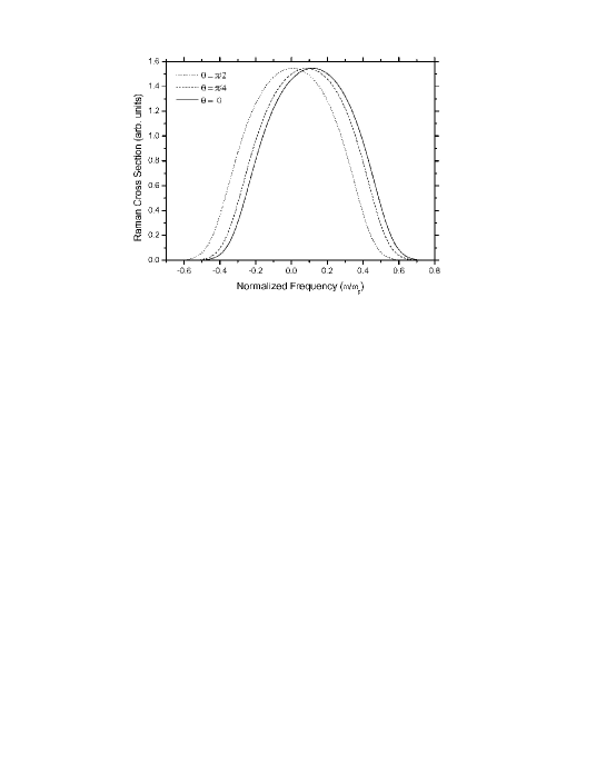
Figure 8: The Raman band due to scattering by the single-particle elementary excitations: $\mathcal{E}=$ 100 kV/cm, $Q=1.8\times 10^{5}$cm^-1, the thermodynamic state as characterized by Figs. 6 and 7 for the given $\mathcal{E}$, and the three scattering angles, $\theta=0$ (full line), $\theta=\pi/4$ (dashed line), and $\theta=\pi/2$ (dotted line). After Ref. [65].

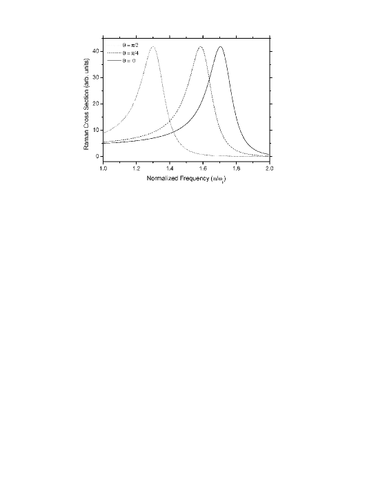
Figure 9: The Raman band due to scattering by the plasma excitation: same specifications as in the caption to Fig. 8, but for $Q=5\times 10^{4}$cm^-1. After Ref. [65].

Let us consider the case of GaN in the steady-state thermodynamic conditions indicated in Figs. 6 and 7, in the case: $\mathcal{E}=100$ kV/cm, and three experimental geometries, i.e. three values of the scattering angle $\theta$. The scattering spectrum is composed of two contributions, namely, scattering, in Fig. 8 with $Q=1.8\times 10^{5}$cm^-1, by individual electrons at low $\omega$, and in Fig. 9 scattering, with $Q=5\times 10^{4}$cm^-1, by collective excitations (plasmons) around the plasma frequency $\omega^{2}_{p}=4\pi ne^{2}/\epsilon_{0}m_{e}^{\ast}$. In these Figs. 8 and 9 it can be noticed a shift in the scattering bands, depending on the scattering angle. This is a result of the presence of the term $\mathbf{Q}\cdot\mathbf{v}_{e}$ in Eq. (196), which is null for the experimental geometry in which the momentum transfer $\mathbf{Q}$ is perpendicular to the drift velocity, which is in the direction of the electric field ($\mathbf{v}_{e}=\mathcal{M}_{e}\mathbf{E}$, where $\mathcal{M}_{e}$ is the electron mobility), and maximum when $\mathbf{Q}$ and $\mathbf{v}_{e}$ are parallel. This has a quite interesting consequence, consisting in that the shift in frequency permits a measurement of the drift velocity, and then of the mobility in the conditions of the experiment. If we call $\Delta\omega_{peak}$ the difference of frequencies at the peak positions of the bands for scattering by plasmons, for $\theta=0$ o and $\theta=\pi/2$ (Fig. 9), then $v_{e}=\Delta\omega_{peak}/Q$ and $\mathcal{M}_{e}=v_{e}/\mathcal{E}=\Delta\omega_{peak}/Q\mathcal{E}$.

VII Final Remarks

We have presented a Response Function Theory, accompanied of a Fluctuation Dissipation Theorem, and a Theory of Scattering adapted to deal with systems arbitrarily away from equilibrium, including situations of time and space experimental resolution.

Such theory was built within the framework of a Gibbs-style Non-Equilibrium Statistical Formalism. The general form of the generalized susceptibility (space and time dependent) is obtained in the form of space and time dependent correlation functions defined over the nonequilibrum ensemble. Moreover it is dependent on the variables that characterized the nonequilibrium thermodynamic state of the system. Therefore, the generalized susceptibility of the corresponding experimental situation is coupled to the equations of evolution of the nonequilibrium thermodynamic variables. It is also presented the method eventually useful for calculations, of nonequilibrium thermodynamic Green functions, that is, the extension to arbitrary nonequilibrium conditions of Bogoliubov-Tyblikov thermodynamic Green functions.

A Fluctuation-Dissipation theorem in the context of the Nonequilibrium Ensemble Formalism has been presented in Section III (see also subsection IV.A), which is an extension to arbitrary nonequilibrium conditions of Kubo’s one.

In Section V we have presented a Theory of Scattering appropriate for scattering experiments done on systems which are arbitrarily away from equilibrium. A space and time dependent scattering cross section is obtained, which, as in the case of the generalized susceptibility of Response Function, is dependent on the nonequilibrium thermodynamic state of the system, and then the scattering cross section is coupled to the equations of evolution of the nonequilibrium variables.

Finally, in section VI we have presented some illustrative examples of the working of the theory in the analysis of several experimental situations, namely, in ultrafast laser spectroscopy and charge transport in doped polar semiconductors.

Acknowledgments: The authors would like to acknowledge partial financial support received from the São Paulo State Research Agency (FAPESP) and the Brazilian National Research Council (CNPq): The authors are CNPq Research Fellows.

Appendix A The Nonequilibrium Statistical Operator

Construction of nonequilibrium statistical ensembles, that is, a Nonequilibrium Statistical Ensemble Formalism, NESEF for short [8-11], consisting in, basically, the derivation of a nonequilibrium statistical operator (probability distribution in the classical case) has been attempted along several lines. In a brief summarized way we descrive the construction of NESEF within a heuristic approach, and, first, it needs to be noticed that for systems away form equilibrium, several important points need to be carefully taken into account in each case under consideration:

1. The choice of the basic variables (a wholly different choice than in equilibrium when it suffices to take a set of those which are constants of motion), which is to be based on an analysis of what sort of macroscopic measurements and processes are actually possible, and moreover, one is to focus attention not only on what can be observed but also on the character and expectative concerning the equations of evolution for these variables [11,66]. We also notice that even though at the initial stage we would need to introduce all the observables of the system, an eventually variances, as time elapses more and more contracted descriptions can be used when it enters into play Bogoliubov’s principle of correlation weakening and the accompanying hierarchy of relaxation times [67].

2. The question of irreversibility (or Eddington’s arrow of time) on what Rudolf Peierls stated that: ”In any theoretical treatment of transport problems, it is important to realize at what point the irreversibility has been incorporated. If it has not been incorporated, the treatment is wrong. A description of the situation that preserves the reversibility in time is bound to give the answer zero or infinity for any conductivity. If we do not see clearly where the irreversibility is introduced, we do not clearly understand what we are doing” [68].

3. Historicity needs be introduced, that is, the idea that it must be incorporated all the past dynamics of the system (or historicity effects), all along the time interval going from a starting description of the macro-state of the sample in the given experiment, say at $t_{0}$, up to the time $t$ when a measurement is performed. This is a quite important point in the case of dissipative systems as emphasized among others by John Kirkwood, Green, Robert Zwanzig and Hazime More [15-19]. It implies in that the history of the system is not merely the series of events in which the system has been involved, but it is the series of transformations along time by which the system progressively comes into being at time $t$ (when a measurement is performed), through the evolution governed by laws of mechanics. [69]

Concerning the question of the choice of the basic variables, differently to the case in equilibrium, immediately after the open system of $N$ particles, in contact with external sources and reservoirs, has been driven out of equilibrium, it would be necessary to describe its state in terms of all its observables and, eventually, introducing direct and cross-correlation. But, as time elapses Bogoliubov’s principle of correlation weakening allow us to introduced increasing contractions of descriptions. Let us say that we can introduce a description based on the observables $\{\hat{P}_{j}\}$, $j=1,2,...,n$, on which depends the noneuilibrium statistical operator.

On the question of irreversibility Nicolai S. Krylov [21] considered that there always exists a physical interaction between the measured system and the external world that is constantly ”jolting” the system out of its exact microstate. Thus, the instability of trajectories and the unavoidable finite interaction with the outside would guarantee the working of a ”crudely prepared” macroscopic description. In the absence of a proper way to introduce such effect, one needs to resort to the interventionist’s approach, which is grounded on the basis of such ineluctable process of randomization leading to the asymmetric evolution of the macro-state.

The ”intervention” consists into introducing in the Liouville equation of the statistical operator, of the otherwise isolated system, a particular source accounting for Krylov’s ”jolting” effect, in the form (written for the logarithm of the statistical operator)

$$\frac{\partial}{\partial t}\ln\Re_{\varepsilon}(t)+\frac{1}{i\hbar}[\ln\Re_{\varepsilon}(t),\hat{H}]=-\varepsilon[\ln\Re_{\varepsilon}(t)-\ln\bar{\Re}(t,0)],$$ (209)

where $\varepsilon$ (kind of reciprocal of a relaxation time) is taken to go to $+0$ after the calculations of average values has been performed. Such mathematically inhomogeneous term, in the otherwise normal Liouville equation, implies in a continuous tendency of relaxation of the statistical operators towards a referential distribution, $\bar{\Re}$, which, as discussed below, represents an instantaneous quasi-equilibrium condition.

We can see that Eq. (A.1) consists of a regular Liouville equation but with an infinitesimal source, which provides Bogoliubov’s symmetry breaking of time reversal and is responsible for disregarding the advanced solutions [8,11,70]. This is described by a Poisson distribution and the result at time $t$ is obtained by averaging over all $t^{\prime}$ in the interval $(t_{0},t)$, once the solution of Eq. (A.1) is

$$\Re_{\varepsilon}(t)=\exp\left\{-\hat{S}(t,0)+\int\limits_{t_{0}}^{t}dt^{\prime}e^{\varepsilon(t^{\prime}-t)}\frac{d}{dt^{\prime}}\hat{S}(t^{\prime},t^{\prime}-t)\right\},$$ (210)

where

$$\hat{S}(t,0)=-\ln\bar{\Re}(t,0),$$ (211)

$$\hat{S}(t^{\prime},t^{\prime}-t)=\exp\left\{-\frac{1}{i\hbar}(t^{\prime}-t)\hat{H}\right\}\hat{S}(t^{\prime},0)\exp\left\{\frac{1}{i\hbar}(t^{\prime}-t)\hat{H}\right\},$$ (212)

and the initial-time condition at time $t_{0}$, when the formalism begins to be applied, is

$$\Re_{\varepsilon}(t_{0})=\bar{\Re}(t_{0},0).$$ (213)

In $\bar{\Re}$ and $\hat{S}$, the first time variable in the argument refers to the evolution of the nonequilibrium thermodynamic variables and the second to the time evolution of the dynamical variables, both of which have an effect on the operator.

This time $t_{0}$, of initiation of the statistical description, is usually taken in the remote past ($t_{0}\rightarrow-\infty$) introducing an adiabatic switching-on of the relaxation process, and in Eq. (A.2) the integration in time in the interval $(t_{0},t)$ is weighted by the kernel $\exp\{\varepsilon(t^{\prime}-t)\}$. The presence of this kernel introduces a kind of evanescent history as the system macro-state evolves toward the future from the boundary condition of Eq. (A.5) at time ($t_{0}\rightarrow-\infty$) a fact evidenced in the resulting kinetic theory [8-11,14,17] which clearly indicates that it has been introduced a fading memory of the dynamical process. It can be noticed that the statistical operator can be write in the form

$$\Re_{\varepsilon}(t)=\bar{\Re}(t,0)+\Re^{\prime}_{\varepsilon}(t)\;.$$ (214)

involving the auxiliary probability distribution $\bar{\Re}(t,0)$, plus $\Re^{\prime}_{\varepsilon}(t)$ which contains the historicity and irreversibility effects. Moreover, in most cases we can consider the system as composed of the system of interest (on which we are performing an experiment) in contact with ideal reservoirs. Thus, we can write

$$\bar{\Re}(t,0)=\bar{\rho}(t,0)\times\rho_{R}\;.$$ (215)

and

$$\Re_{\varepsilon}(t)=\rho_{\varepsilon}(t)\times\rho_{R}\;,$$ (216)

where $\rho_{\varepsilon}(t)$ is the statistical operator of the nonequilibrium system, $\bar{\rho}$ the auxiliary one, and $\rho_{R}$ the stationary one of the ideal reservoirs, with $\rho_{\varepsilon}(t)$ given then by

$$\rho_{\varepsilon}(t)=\exp\left\{-\hat{S}(t,0)+\int\limits_{-\infty}^{t}dt^{\prime}e^{\varepsilon(t^{\prime}-t)}\frac{d}{dt^{\prime}}\hat{S}(t^{\prime},t^{\prime}-t)\right\}\;,$$ (217)

having the initial value $\bar{\rho}(t_{0},0)$ ($t_{0}\rightarrow-\infty$), and where

$$\hat{S}(t,0)=-\ln\bar{\rho}(t,0)\;,$$ (218)

Finally, it needs be provided the auxiliary statistical operator $\bar{\rho}(t,0)$. It defines an instantaneous distribution at time $t$, which describes a ”frozen” equilibrium defining at such given time the macroscopic state of the system, and for that reason is sometimes dubbed as the quasi-equilibrium statistical operator. On the basis of this (or, alternatively, via the extremum principle procedure [11,71-76], and considering the description of the non-equilibrium state of the system in terms of the basic set of dynamical variables $\hat{P}_{j}$, the reference or instantaneous quasi-equilibrium statistical operator is taken as a canonical-like one given by

$$\bar{\rho}(t,0)=\exp\{-\phi(t)-\sum\limits_{j}^{n}F_{j}(t)\hat{P}_{j}\}\;,$$ (219)

in the classical case, with $\phi(t)$ ensuring the normalization of $\bar{\rho}$ and playing the role of a kind of a logarithm of a partition function, say, $\phi(t)=\ln\bar{Z}(t)$. Moreover, in this Eq. (A.11), $F_{j}$ are the nonequilibrium thermodynamic variables associated to each kind of basic dynamical variables $\hat{P}_{j}$. The nonequilibrium thermodynamic space of states is composed by the basic variables $\{Q_{j}(t)\}$ consisting of the averages of the $\{\hat{P}_{j}\}$ over the nonequilibrium ensemble, namely

$$Q_{j}(t)=Tr\{\hat{P}_{j}\rho_{\varepsilon}(t)\}\,,$$ (220)

which are then functionals of the $\{F_{j}(t)\}$ and there follow the equations of state

$$Q_{j}(t)=-\frac{\delta\phi(t)}{\delta F_{j}(t)}=-\frac{\delta\ln\bar{Z}(t)}{\delta F_{j}(t)}\,,$$ (221)

where $\delta$ stands for functional derivative.

Moreover

$$\bar{S}(t)=Tr\{\hat{\bar{S}}(t,0)\bar{\rho}(t,0)\}=-Tr\{\bar{\rho}(t,0)\ln\bar{\rho}(t,0)\}\,,$$ (222)

is the so-called informational entropy characteristic of the distribution $\bar{\rho}$, a functional of the basic variables $\{Q_{j}(t)\}$, and it is verified the alternative form of the equations of state given by

$$-\frac{\delta\bar{S}(t)}{\delta Q_{j}(t)}=F_{j}(t)\,,$$ (223)

References

• (1) Kubo R 1978 Oppening address at the Oji seminar Prog. Theor. Phys. (Japan) 64
• (2) Stix S 2001 Little big science: an overview, and articles thereafter Scientific American 285(3) 26
• (3) Family F and Vicsek T 1991 Dynamics of Fractal Surfaces (World Scientific, Singapore)
• (4) Luzzi R, Vasconcellos A R and Ramos J G 2007 Non-equilibrium statistical mechanics of complex systems: an overview Riv. Nuovo Cimento 30(3) 95
• (5) Renyi A 1961 On measures of entropy and information (Proc. 4th Berkeley Symposium Math. Stat. Prob. vol 1) p 547.
• (6) Renyi A 1970 Probability Theory (North Holland, Amsterdam, The Netherlands)
• (7) Jizba P and Arimitzu T 2004 The world according to Renyi Ann. Phys. (NY) 312 17
• (8) Zubarev D N 1974 Non Equilibrium Statistical Thermodynamics (Consultants Bureau, New York, USA)
• (9) Zubarev D N, Morozov V and Röpke G 1996 Statistical Mechanics of Non Equilibrium Processes I (Academie Verlag-Wiley VCH, Berlin, Germany)
Zubarev D N, Morozov V and Röpke G 1997 Statistical Mechanics of Non Equilibrium Processes II (Academie Verlag-Wiley VCH, Berlin, Germany)
• (10) Akhiezer A and Peletminskii S 1981 Methods of Statistical Physics (Pergamon, Oxford, UK)
• (11) Luzzi R, Vasconcellos A R and Ramos J G 2002 Predictive Statistical Mechanics: A Non-Equilibrium Ensemble Formalism (Kluwer Academic, Dordrecht, The Netherlands)
Luzzi R, Vasconcellos A R and Ramos J G 2006 Riv. Nuovo Cimento 29(2), 1-82
• (12) Kalos M H and Whitlock P A 2007 Monte Carlo Methods (Wiley-Interscience, New York, USA)
• (13) Adler B J and Tildesley D J 1987 Computer Simulation of Liquids (Oxford Univ. Press, Oxford, UK)
• (14) Lauck L, Vasconcellos A R and Luzzi R 1990 A non-linear quantum transport theory Physica A 168 789
• (15) Kirkwood J G 1946 The statistical mechanical theory of transport processes: I. General Theory J. Chem. Phys. 14 180
• (16) Green M S 1952 Markoff random processes and the statistical mechanics of time-dependent phenomena J. Chem. Phys. 20 1281
• (17) Mori H, Oppenheim I and Ross J 1962 Some topics in quantum statististics in Studies in Statistical Mechanics I edited by J de Boer and G E Uhlenbeck (North Holland, Amsterdam, The Netherlands)
• (18) Mori H 1965 Transport, collective motion, and Brownian motion Progr. Theor. Phys. (Japan) 33 423
• (19) Zwanzig R 1961 Statistical mechanics of irreversibility in: Lectures in Theoretical Physics vol 3 edited by W E Brittin, B W Downs and J Downs (Wiley-Interscience, New York, USA)
• (20) Salam A, Vladimorov V S and Logunov A A 1993 Tribute in memoriam of Nicolai N. Bogoliubov Theor. Math. Phys. 92 817
• (21) Krylov N S 1979 Works on The Foundations of Statistical Mechanics (Princeton Univ. Press, Princeton, USA)
• (22) Peletminski S V and Yatsenko A A 1968 Contribution to the quantum theory of kinetic and relaxation processes JETP 26 773
• (23) Zubarev D N and Kalashnikov V P 1970 Extremal properties of the nonequilibrium statistical operator Theor. Math. Phys. 96 108
• (24) Jaynes E T 1983 in: E. T. Jaynes: papers on probability, statistics and statistical physics edited by R. D. Rosenkrantz (Reidel, Dordrecht, The Netherlands)
• (25) Jaynes E T 1986 Predictive statistical mechanics in: Frontiers of Non Equilibrium Statistical Physics edited by G. T. Moore and M. O. Scully, (Plenum, New York, USA) 33-55
• (26) Shannon C E 1948 A mathematical theory of communication Bell Sys. Tech. J. 27 379-423
• (27) Shannon C E and W. Weaver 1949 The Mathematical Theory of Communication (Univ. Illinois Press, Urbana, USA)
• (28) Martin P C 1968 Measurements and Correlation Functions, in Many-Body Physics edited by C D Witt and R Balian (Gordon and Breach, New York, USA) 37-136
• (29) Hove L 1954 Correlations in space and time and Born approximation scattering in systems of interacting particles Phys. Rev. 95 249 and 1374
• (30) Kreuzer H J 1981 Non Equilibrium Thermodynamics and its Statistical Foundations (Claredon, Oxford, UK)
• (31) Kalashnikov V P 1971 Response to a mechanical perturbation and the Green’s functions for nonequilibrium systems Theor. Math. Phys. 9 1003
• (32) Kalashnikov V P 1978 Equations of motion, Green’s functions, and thermodynamic relations in theories of linear relaxation with various sets of macroscopic variables Theor. Math. Phys. 35 362
• (33) Luzzi R and Vasconcellos A R 1980 Response function theory for far-from-equilibrium statistical systems J. Stat. Phys. 23 539
• (34) Nyquist H 1928 Themal agitation of electric charge conductors Phys. Rev. 32 110
• (35) Callen H B and Welton T A 1951 Irreversibility and generalized noise Phys. Rev. 83 34
• (36) Kubo R 1957 Statistical mechanics theory of irreversible processes J. Phys. Soc. Japan 12 570
Kubo R 1966 The fluctuation-dissipation theorem Rep. Prog. Phys. 29 255
• (37) Zon R and Cohen E G D 2003 Extension of the Fluctuation Theorem Phys. Rev. Lett. 91 110601
• (38) Evans D J and Searles D J 2002 The Fluctuation Theorem Adv. Phys. 51 1529
• (39) Luzzi R, Vasconcellos A R, Casas-Vazquez J and Jou D 1997 Thermodynamic variables in the context of a nonequilibrium statistical approach J. Chem. Phys. 107 7383
• (40) Luzzi R, Vasconcellos A R, Casas-Vazquez J and Jou D 1997 Characterization and measurements of a nonequilibrium temperature-like variable in irreversible thermodynamics Physica A 234 699
• (41) Luzzi R, Vasconcellos A R, Casas-Vazquez J and Jou D 1998 On the selection of the state space in nonequilibrium thermodynamics Physica A 248 111
• (42) Rodrigues C G, Vasconcellos A R and Luzzi R 2000 A kinetic theory for nonlinear quantum transport Transp. Theor. Stat. Phys. 29 733
• (43) Kalashnikov V P 1972 Response to a mechanical pertubation and the Green’s function for nonequilibrium system Theor. Math. Phys. 9 1003
• (44) Kalashnikov V P 1978 Equations of motion, Green’s functions and thermodynamic relations in theories of linear relaxation Theor. Math. Phys. 35 362
• (45) Zubarev D N 1960 Double-time Green’s functions in statistical mechanics Uspekhi 3 320
• (46) Tyablikov V L 1974 Methods in The Quantum Theory of Magnestism (Plenum, New York, USA)
• (47) Madureira J R, Vasconcellos A R, Luzzi R and Lauck L 1998 Markovian kinetic equations in a nonequilibrium statistical ensemble formalism Phys. Rev. E 57 3637
• (48) Luzzi R and Vasconcellos A R 1981 Time-resolved Raman spectra of photoexcited semiconductor plasma J. Raman Spectrosc. 10 28
• (49) Vasconcellos A R and Luzzi R 1983 Plasma-phonon coupling effects in picosecond Raman scattering of nonequilibrium semiconductor plasma J. Raman Spectrosc. 14 39
• (50) Hove L 1961 in Quantum Theory of Many-Particle Systems edited by L van Hove, N M Hugenholtz and L P Howland (Benjamin, New York, USA)
• (51) Cho G L, Kütt W and Kurz H 1990 Subpicosecond time-resolved coherent-phonon oscillations in GaAs Phys. Rev. Lett. 65 764
• (52) Albrecht W, Kruse T and Kurz H 1992 Time-resolved observation of coherent phonons in superconducting YBa2Cu3O7-δ thin-films Phys. Rev. Lett. 69 1451-1454
• (53) Pfeifer T, Kütt W and Scholz R 1992 Generation and detection of coherent optical phonons in germanium Phys. Rev. Lett. 69 3248
• (54) Scholz R, Pfeifer T and Kurz H 1993 Density-matrix theory of coherent phonon oscillation in germanium Phys. Rev. B 47 16229
• (55) Zeiger H J, Vidal J, Cheng T. K, Ippen E P, Dresselhaus G and Dresselhaus M S 1992 Theory of displacive excitation of coherent phonons Phys. Rev. B 45 768
• (56) Kutnevsov A V and Stanton C J 1994 Theory of coherent phonon oscillation in semiconductors Phys. Rev. Lett. 73 3243
• (57) Vasconcellos A R, Luzzi R and Madureira A J 2000 Optical properties of semiconductors via pump probe experiments: statistical thermodynamic approach, hot plasma and coherent phonon states J. Phys.: Condens. Matter 12 5325
• (58) Algarte A C, Vasconcellos A R and Luzzi R 1996 Ultrafast kinetics of evolution of optical phonons in a photoinjected highly excited plasma in semiconductors Phys. Rev. B 54 11311
Algarte A C, Vasconcellos A R and Luzzi R 1996 Ultrafast phenomena in the photoinjected plasma in semiconductors Braz. J. Phys. 26 543
• (59) Rodrigues C G, Vasconcellos A R, Luzzi R 2005 Ultrafast relaxation kinetics of photoinjected plasma in III-nitrides. J. Phys. D: Appl. Phys. 38 3584-3589
Rodrigues C G, Vasconcellos A R, Luzzi R 2006 Nonlinear transport in n-III-nitrides: selective amplification and instability of the LO-phonon system Solid State Commun. 140 135-140
• (60) Wolff P 1969 in Light Scattering Spectra of Solids edited by G B Wright (Springer, New York, USA)
• (61) Mooradian A 1969 in Light Scattering Spectra of Solids edited by G. B. Wright (Springer, New York, USA)
• (62) Silva A A P, Algarte A C, Vasconcellos A R and Luzzi R 2001 Relaxation dynamics of hot carriers and phonons in semiconductors: Influence of the excitation conditions J. Appl. Phys. 90 3973
• (63) Johnson N M, Nurmikko A V and DenBoars S P 2000 Blue Diode Lasers Phys. Today 53(10) 31
Rodrigues C G, Silva A A P, Silva C A B, Vaconcellos A R, Ramos J G, Luzzi R 2010 The role of nonequilibrium thermo-mechanical statistics in modern technologies and industrial processes: an overview Braz. J. Phys. 40 63-91
• (64) Rodrigues C G, Vasconcellos A R and Luzzi R 2009 Optical properties of III-nitrides in electric fields Eur. Phys. J. B 72(1) 67
• (65) Neto A V A, Vasconcellos A R, Freire V N and Luzzi R, Ultrafast carrier transport in semiconductors studied via optical spectroscopy: application to III-nitrides, unpublished.
• (66) Zwanzig R 1981 Where we go from here? in Perspectives in Statistical Mechanics edited by H J Raveché (North Holland, Amsterdam, The Netherlands)
• (67) Bogoliubov N N 1962 Problems of a dynamical theory in statistical physics in Studies in Statistical Physics edited by J de Boer and G E Uhlenbeck (North Holland, Amsterdam, The Netherlands)
• (68) Peierls R 1974 Some simple remarks on the basis of transport theory, in transport phenomena in Lecture Notes in Physics vol. 31 edited by J Ehlers, K Hepp and H A Weidenmuller (Springer, Berlin, Germany)
• (69) Mori H, Oppenheim I and Ross J 1962 Some topics in quantum statistics in Studies in Statistical Mechanics I edited by J de Boer and G E Uhlenbeck (North Holland, Amsterdam, The Netherlands)
• (70) Bogoliubov N N 1967 Lectures in Quantum Mechanics vol. 1 (Gordon and Breach, New York, USA)
Bogoliubov N N 1970 Lectures in Quantum Mechanics vol. 2 (Gordon and Breach, New York, USA)
• (71) Elsasser W M 1937 On quantum measurements and the role of the uncertainty relations in statistical mechanics Phys. Rev. 52 987
• (72) Jaynes E T 1993 in Physics and Probability edited by W T Grandy and P W Milonni (Cambridge Univ. Press, Cambridge, UK) 261-275.
• (73) Jaynes E T 1991 in Maximum Entropy and Bayesian Methoods edited by W.T. Grandy and L. H. Schick (Kluwer Academic Dordrecht, The Netherlands) 1-13.
• (74) Robertson B 1966 Equations of motion in nonequilibrium statistical mechanics Phys. Rev. 144, 151-161
Robertson B 1967 Equations of motion in nonequilibrium statistical mechanics. II. Energy transport Phys. Rev. 160 175-183
• (75) Jaynes E T 2002 Probability Theory as Extended Logic (Cambridge Univ. Press, Cambridge, UK)
• (76) Bricmont J 2001 in Chance in Physics edited by J. Bricmont et al. (Springer, Heidelberg, Germany)
Bricmont J 1995 Science of chaos or chaos in science? Physicalia Magazine 17 159-208
Bricmont J 1996 in The Flight from Science and Reason, Annals New York Academy of Sciences vol. 775 (NYAS, New York, USA) 131-175