Development and application of a particle-particle particle-mesh Ewald method for dispersion interactions

Abstract

For inhomogeneous systems with interfaces, the inclusion of long-range dispersion interactions is necessary to achieve consistency between molecular simulation calculations and experimental results. For accurate and efficient incorporation of these contributions, we have implemented a particle-particle particle-mesh (PPPM) Ewald solver for dispersion ($r^{-6}$) interactions into the LAMMPS molecular dynamics package. We demonstrate that the solver’s $\mathcal{O}(N\log N)$ scaling behavior allows its application to large-scale simulations. We carefully determine a set of parameters for the solver that provides accurate results and efficient computation. We perform a series of simulations with Lennard-Jones particles, SPC/E water, and hexane to show that with our choice of parameters the dependence of physical results on the chosen cutoff radius is removed. Physical results and computation time of these simulations are compared to results obtained using either a plain cutoff or a traditional Ewald sum for dispersion.

I Introduction

Despite their weak $r^{-6}$ scaling, dispersion forces “play a role in a host of important phenomena such as adhesion; surface tension; physical adsorption; wetting; the properties of gases, liquids, and thin films; the strength of solids; the flocculation of particles in liquids; and the structures of condensed macromolecules such as proteins and polymers.”Israelachvili (2011) Unsurprisingly, their contributions to intermolecular interactions are accounted for in the vast majority of the nonbonded potentials applied in molecular simulations. Typically, dispersion interactions are only considered within a cutoff of around 1 nm. For homogeneous systems, the contributions of long-ranged interactions can be estimated efficiently and accurately.Allen and Tildesley (1987) For inhomogeneous systems, however, these corrections are inaccurate, and computational requirements has precluded the inclusion of long-range dispersion interactions, even though, as can be seen from the applications above, they are especially relevant for these systems. The necessity of incorporating the long-range effects of dispersion forces has been shown in numerous studies on surface simulationsChapela, Saville, and Thompson (1977); Blokhuis et al. (1995); Guo, Peng, and Lu (1997); Guo and Lu (1997); Mecke, Winkelmann, and Fischer (1997); Janeček (2006); López-Lemus et al. (2006); in ’t Veld, Ismail, and Grest (2007); Ismail et al. (2007) of which only some are referenced here, but also in simulations near the critical point,Ou-Yang et al. (2005) and in simulations of protein-ligand binding.Shirts et al. (2007)

Various correction methods have been proposed for incorporating long-range dispersion contributions. Most molecular simulation packages already include energy and pressure corrections assuming homogeneous systems. Similar “on-line” methods that can be applied during simulations have been presented by Guo et al.Guo, Peng, and Lu (1997); Guo and Lu (1997) for Monte Carlo and by Mecke et al.Mecke, Winkelmann, and Fischer (1997) and JanečekJaneček (2006) for molecular dynamics (MD) simulations. Chapela et al.Chapela, Saville, and Thompson (1977) and Blokhuis et al. Blokhuis et al. (1995) have developed a tail correction for simulated surface tensions that can be added after the end of the simulations. The aformentioned correction methods are applicable only to simulations with planar interfaces. The use of a twin-range cutoff has been proposed by Lagüe et al.Lagüe, Pastor, and Brooks (2003) Wu and BrooksWu and Brooks (2005) present the isotropic periodic sum for electrostatic interactions, but the method can be extended to incorporate long-range dispersion forces.

An alternative to these “correction”-based schemes is to include the long-range interactions explicitly using Ewald summation, which was originally developed for the treatment of Coulomb forces.Ewald (1921) This method was developed for dispersion by Williams,Williams (1970) Perram,Perram, Petersen, and Leeuw (1988) and Karasawa and Goddard,Karasawa and Goddard (1989) and later applied to surface simulations by López-Lemus et al.,López-Lemus et al. (2006) Grest and co-workers,in ’t Veld, Ismail, and Grest (2007); Ismail et al. (2007) Ou-Yang et al.,Ou-Yang et al. (2005) and Alejandre and Chapela.Alejandre and Chapela (2010) Among the previously mentioned methods for treating long-range dispersion interactions, the Ewald sum is usually the most accurate, most reliable, and most versatile. However, its $\mathcal{O}(N^{3/2})$ scalingPerram, Petersen, and Leeuw (1988) prohibits its application in large-scale simulations. This problem can be overcome by applying grid-based Ewald summation methods,Hockney and Eastwood (1988); Darden, York, and Pedersen (1993); Essmann et al. (1995); Deserno and Holm (1998a) whose scaling, because of the use of fast Fourier transforms (FFT), is $\mathcal{O}(N\log N)$. While frequently used for Coulomb interactions, such methods have also been applied to dispersion interaction by Essman et al.Essmann et al. (1995) and Shi et al.Shi, Sinha, and Dhir (2006) In the former work, the dispersion part is only adressed very briefly for particle-mesh Ewald (PME), and not for PPPM. The latter puts a stronger focus on the PPPM and dispersion interactions. We feel, however, that the description is incomplete; for example, the equations for the energy and virial and the exact formulation of the true reference force are not given. Furthermore, we provide a simpler method for calculating the pressure tensor required for calculating surface tensions, and outline reasons why their simulated surface tensions do not agree with other reported results for SPC/E water.

We present the results of the development and implementation of a particle-particle particle-mesh (PPPM) solver for $r^{-6}$ dispersion interaction in the LAMMPSPlimpton (1995) molecular dynamics package. The theory is given in Section II. Error estimates for the real and reciprocal space contributions, as well as a discussion on the limits of the error estimate, are presented in section III. The scaling behavior of the developed algorithm is presented in Section IV. We have performed a variety of interfacial simulations, as long-range dispersion interactions are known to have a significant effect on simulated surface tensions. The theory for calculating surface tensions is briefly reviewed in Section V. A set of parameters for performing successful simulations with the PPPM for dispersion is determined in Section VI. We use these parameters in Section VII to study the surface tension of Lennard-Jones (LJ) particles, hexane, and SPC/E water. Section VIII contains a brief comparison of the simulation time of different solvers. We summarize our findings in the final section.

II Formulation of the mesh-based dispersion sum

Excellent reviews on traditional and mesh-based Ewald sums are given by Hockney and Eastwood,Hockney and Eastwood (1988) Essmann et al.,Essmann et al. (1995) and Deserno and Holm.Deserno and Holm (1998a) Karasawa et al.Karasawa and Goddard (1989) provide a comprehensive description of the traditional Ewald sum for dispersion interactions. To make the presentation as self-contained as possible, we provide a complete summary of the PPPM algorithm as applied to dispersion interactions, compiled from the above references.

Because of its physical origin in the overlap of electron hulls, the repulsive (often $r^{-n}$, where typically $n\geq 9$) part of pair potentials is very short-ranged and can be neglected beyond a typical cutoff length of 1 nm. We therefore exclude the repulsive term from further consideration. The attractive part between two atomic sites of some commonly used pair potentials, such as the LJ or Buckingham potential,Stone (1997) can be expressed as

$$u_{\mathrm{attr}}(r_{ij})=-\frac{C_{ij}}{r^{6}},$$ (1)

where $r$ is the distance between particles $i$ and $j$ and $C_{ij}$ is the dispersion coefficient describing the strength of the interaction. The goal of the Ewald summation is to split this potential into a fast-decaying potential, whose contribution can be neglected beyond a cutoff, and a slowly decaying potential, whose contribution can be accounted for in Fourier space, as shown in Figure 1. Its calculation requires a Fourier transform of the dispersion coefficients into the reciprocal space.

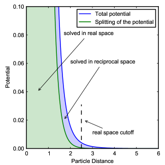
Figure 1: Total potential and split potential for $r^{-6}$. When not using the Ewald sum, the whole area under the blue curve is solved in real space, whereas only the area under the green curve is solved in real space when using the Ewald sum. The error in the calculation is related to the area under the curves beyond the cutoff. Using the Ewald technique is thus more accurate.

The benefit of mesh-based Ewald methods, such as PPPM, is that the dispersion coefficients are distributed onto a grid, which permits application of the FFT for the calculation of the dispersion coefficient density. The calculation of the mesh Ewald sums in reciprocal space requires additional steps. The dispersion coefficients have to be distributed onto a grid and transformed into reciprocal space to calculate their interactions in Fourier space. The resulting potential must then be derived and backinterpolated onto the atomic sites to obtain the forces.

The dispersion energy of a system with the potential above is given byKarasawa and Goddard (1989); Deserno and Holm (1998a)

$$E_{6}= \frac{\beta^{6}}{2}\sum_{i,j}C_{ij}\left(1+\beta^{2}r_{ij}^{2}+\frac{\beta^{4}r_{ij}^{4}}{2}\right)\frac{\exp\left(-r_{ij}^{2}\beta^{2}\right)}{\beta^{6}r_{ij}^{6}}$$

$$+\frac{1}{2V}\sum_{\mathbf{k}\in\mathbb{M}}\hat{G}(\mathbf{k})\hat{\mathcal{S}}_{6}^{2}(\mathbf{k})$$

$$+\frac{\pi^{3/2}\beta^{3}}{6V}\sum_{i,j}C_{ij}-\frac{\beta^{6}}{12}\sum_{i}C_{ii},$$ (2)

where $\beta$ is the Ewald parameter for dispersion interactions, $r_{ij}$ is the distance between particle $i$ and the nearest image of particle $j$, and $V$ is the volume of the simulation box. $\hat{G}$ is the optimum dispersion influence function, which has a different form than the electrostatic influence function. $\hat{\mathcal{S}}_{6}^{2}$ is a function of the location and strength of the dispersion sites. The $\mathbf{k}$ vectors form the discrete set $\left\{2\pi\mathbf{n}/L\right\}$, where $L$ is the length of the box vectors and the components of ${\bf n}=(n_{x},n_{y},n_{z})$ are integer values that are zero for the center node of the grid. The first sum in equation II is over all pairs of atoms. However, as the potential decays quickly with increasing interparticle distance, it is only evaluated for particles whose $r_{ij}$ is smaller than a chosen cutoff. The second sum is over the reciprocal vectors of all grid points.

The expression for the optimum influence function, which minimizes the error in the calculated forces, isHockney and Eastwood (1988); Deserno and Holm (1998a)

$$\hat{G}(\mathbf{k})=\frac{\mathbf{\tilde{D}}(\mathbf{k})\sum_{\mathbf{m}\in\mathbb{Z}^{3}}\tilde{U}^{2}\left(\mathbf{k}+\frac{2\pi}{h}\mathbf{m}\right)\mathbf{\tilde{R}}\left(\mathbf{k}+\frac{2\pi}{h}\mathbf{m}\right)}{|\tilde{\mathbf{D}}(\mathbf{k})|^{2}\left[\sum_{\mathbf{m}\in\mathbb{Z}^{3}}\tilde{U}^{2}\left(\mathbf{k}+\frac{2\pi}{h}\mathbf{m}\right)\right]^{2}},$$ (3)

with

$$\tilde{U}(\mathbf{k})=\frac{\tilde{W}^{(P)}(\mathbf{k})}{V},$$ (4)

where $P$ is the interpolation order and

$$\tilde{W}^{(P)}=h^{3}\left(\frac{\sin(k_{x}h/2)}{k_{x}h/2}\frac{\sin(k_{y}h/2)}{k_{y}h/2}\frac{\sin(k_{z}h/2)}{k_{z}h/2}\right)^{P}$$ (5)

is the Fourier transform of the interpolation function $W^{(P)}$, which is described, for example, in Ref. Deserno and Holm, 1998a, and $h$ is the grid spacing. $\mathbf{\tilde{D}}$ is the Fourier transform of the differentiation operator required for the force calculation. In this study, we use differentiation in Fourier space

$$\mathbf{\tilde{D}}(\mathbf{k})=i\mathbf{k}.$$ (6)

$\mathbf{\tilde{R}}$ is the Fourier transform of the true reference force and can, for dispersion interaction, be calculated asDeserno and Holm (1998a); Essmann et al. (1995)

$$\mathbf{\tilde{R}}(\mathbf{k})=i\mathbf{k}\frac{\pi^{3/2}\beta^{3}}{3}\left[\left(1-2b^{2}\right)e^{-b^{2}}+2b^{3}\sqrt{\pi}\mathrm{erfc}\left(b\right)\right],$$ (7)

with $b={|\mathbf{k}|}/{2\beta}$.

For our choice of $\tilde{U}$, the denominator in equation 3 can be evaluated analytically, as shown by Hockney and EastwoodHockney and Eastwood (1988) or in a more explicit form by Pollock et al.Pollock and Glosli (1996) The sum in the numerator is usually sufficiently converged when terms with $|\mathbf{m}|\leq 2$ are included. As the influence function is independent of the particle coordinates, it needs to be calculated only at the beginning of a simulation or when the volume has changed.

When the dispersion coefficient of a pair of atoms can be expressed using a geometric mixing rule,

$$C_{ij}=\sqrt{C_{ii}C_{jj}}=c_{i}c_{j},$$ (8)

as in, for example, the OPLS potential,Jorgensen and Tirado-Rives (1988) the function $\hat{\mathcal{S}}_{6}^{2}(\mathbf{k})$ can be expressed as

$$\hat{\mathcal{S}}_{6}^{2}(\mathbf{k})=\hat{S}_{6}(\mathbf{k})\hat{S}_{6}^{*}(\mathbf{k}),$$ (9)

where $\hat{S}_{6}^{*}$ is the complex conjugate of the structure factor $\hat{S}_{6}$, which is the discrete Fourier transform of the dispersion coefficient density $c_{M}$ on the grid points:

$$\hat{S}_{6}(\mathbf{k})=\sum_{\mathbf{r_{p}}\in\mathbb{M}}c_{M}(\mathbf{r_{p}})\exp\left(-i\mathbf{k\cdot r_{p}}\right).$$ (10)

When using an LJ potential, the dispersion coefficients of unlike sites are often determined via the Lorentz-Berthelot mixing rule as

$$C_{ij}=4\sqrt{\epsilon_{i}\epsilon_{j}}\left(\frac{\sigma_{i}+\sigma_{j}}{2}\right)^{6},$$ (11)

where $\epsilon$ and $\sigma$ are LJ parameters. Equation 8 cannot be used in this case; instead, $\hat{\mathcal{S}}_{6}^{2}(\mathbf{k})$ must be calculated byin ’t Veld, Ismail, and Grest (2007)

$$\hat{\mathcal{S}}_{6}^{2}(\mathbf{k})=\sum_{i=0}^{6}\hat{S}_{6,k}(\mathbf{k})\hat{S}_{6,k}^{*}(\mathbf{k}),$$ (12)

with

$$\hat{S}_{6,k}(\mathbf{k})=\sum_{\mathbf{r_{p}}\in\mathbb{M}}c_{k,M}(\mathbf{r_{p}})\exp\left(-i\mathbf{k\cdot r_{p}}\right),$$ (13)

where $c_{k,M}$ is the dispersion coefficient density on the mesh points obtained from interpolating the dispersion coefficients

$$c_{i,k}=\frac{1}{4}\sigma_{i}^{k}\sqrt{\binom{6}{k}\epsilon_{i}}$$ (14)

onto a grid. Because of their symmetry only four of the seven addends in equation 12 have to be calculated. Although the imaginary part of each addend is not necessarily zero, the imaginary parts of the sum will cancel out identically.

Additional steps are required for calculating the mesh-based forces. For $i{\mathbf{k}}$ differentiation, the dispersion field can be calculated asDeserno and Holm (1998a)

$$\mathbf{E}(\mathbf{r_{p}})=-\overleftarrow{\mathrm{FFT}}\left(i\mathbf{k}\frac{1}{V}\hat{S}_{6}\hat{G}\right)(\mathbf{r_{p}}),$$ (15)

where $\overleftarrow{\mathrm{FFT}}$ indicates the reverse fast Fourier transform. The total force on particle $i$, based on the the real and the reciprocal part, can then be calculated asKarasawa and Goddard (1989); Deserno and Holm (1998a)

$$\mathbf{F}_{i}= \sum_{j}C_{ij}\left(\frac{6}{r_{ij}^{8}}+\frac{6\beta^{2}}{r_{ij}^{6}}+\frac{3\beta^{4}}{r_{ij}^{4}}+\frac{\beta^{6}}{r_{ij}^{2}}\right)\times$$

$$\exp\left(-r_{ij}^{2}\beta^{2}\right)\mathbf{r}_{ij}+c_{i}\sum_{\mathbf{r_{p}}\in\mathbb{M}}\mathbf{E}(\mathbf{r_{p}})W(\mathbf{r}_{i}-\mathbf{r_{p}}).$$

It should be noted that equation 15 and the second term in equation II have to be calculated for each of the seven structure factors when the Lorentz-Berthelot mixing rule is used.

The instantaneous stress is given byKarasawa and Goddard (1989)

$$V\Pi_{\alpha\beta}= \frac{1}{2}\sum_{i,j}C_{ij}\left(\frac{6}{r_{ij}^{8}}+\frac{6\beta^{2}}{r_{ij}^{6}}+\frac{3\beta^{4}}{r_{ij}^{4}}+\frac{\beta^{6}}{r_{ij}^{2}}\right)\times$$

$$\exp\left(-r_{ij}^{2}\beta^{2}\right)\mathbf{r}_{ij,\alpha}\mathbf{r}_{ij,\beta}+\frac{1}{2V}\sum_{\mathbf{k}\in\mathbb{M}}\hat{G}(\mathbf{k})\hat{\mathcal{S}}_{6}^{2}(\mathbf{k})\times$$

$$\left(\delta_{\alpha\beta}-\frac{3}{k^{2}}\frac{2b^{3}\sqrt{\pi}\mathrm{erfc}(b)-2b^{2}e^{-b^{2}}}{2b^{3}\sqrt{\pi}\mathrm{erfc}(b)+(1-2b^{2})e^{-b^{2}}}k_{\alpha}k_{\beta}\right)$$

$$+\frac{\pi^{2/3}\beta^{3}}{6V}\sum_{i,j}C_{ij}\delta_{\alpha\beta},$$ (17)

where $\delta_{\alpha\beta}$ is the Kronecker delta.

III Formulation of an Error Measure

Several parameters can be tuned to influence the accuracy of the dispersion PPPM: the chosen cutoff radius $r_{c}$ for the sum in real space, the Ewald parameter $\beta$, the grid size, and the order of the interpolation function for distributing the dispersion coefficient onto a grid. The qualitative influence of the parameters can be understood easily. The real space error arises from truncating the pair potential. Increasing the cutoff radius or the Ewald parameter, which leads to a faster decaying real space potential, increases the accuracy in real space. The precision in reciprocal space depends on the Ewald parameter, the grid spacing, and the interpolation order. Decreasing either of the first two or increasing the latter of these parameters will lead to higher accuracy in the reciprocal space contribution.

To choose the tunable parameters effectively, a more quantitative understanding of the parameters’ influence is required. The following sections present estimates for the error of real and reciprocal space contribution to the forces.

III.1 Error measure for the real-space contribution

To describe the real space error, we extend the derivation of Kolafa and PerramKolafa and Perram (1992) for Coulomb interaction to $r^{-6}$ potentials. The sum of the square of the real-space contribution of the dispersion interaction of the particles beyond the cutoff $r_{c}$ on a single particle can be expressed as

$$\Delta F_{i}^{2} = c_{i}^{2}\sum_{j:r_{ij}>r_{c}}c_{j}^{2}\left(\frac{6}{r_{ij}^{8}}+\frac{6\beta^{2}}{r_{ij}^{6}}+\frac{3\beta^{4}}{r_{ij}^{4}}+\frac{\beta^{6}}{r_{ij}^{2}}\right)^{2}\times$$ (18)

$$\exp\left(-2r_{ij}^{2}\beta^{2}\right)r_{ij}^{2}.$$

Assuming that the particles are randomly distributed beyond the cutoff, the sum can be replaced by an integral to arrive at

$$\Delta F_{i}^{2} = c_{i}^{2}\sum_{j}c_{j}^{2}\frac{1}{V}\int_{r_{c}}^{\infty}\left(\frac{6}{r_{ij}^{6}}+\frac{6\beta^{2}}{r_{ij}^{4}}+\frac{3\beta^{4}}{r_{ij}^{2}}+\beta^{6}\right)^{2}\times$$

$$\exp\left(-2r_{ij}^{2}\beta^{2}\right)4\pi\mathrm{d}r.$$

Using

$$\int_{A}^{\infty}\exp(-Bx^{2})f(x)\mathrm{d}x\approx\exp(-BA^{2})\frac{f(A)}{2BA},$$

which is valid for $B>0$, and

$$\frac{\mathrm{d}(f(x)/2Bx)}{\mathrm{d}x}\leq f(x)$$

for $x\geq A$, we arrive at

$$\Delta F_{i}^{2} = c_{i}^{2}\sum_{j}c_{j}^{2}\frac{\pi\beta^{10}}{Vr_{c}}\left(\frac{6}{r_{c}^{6}\beta^{6}}+\frac{6}{r_{c}^{4}\beta^{4}}+\frac{3}{r_{c}^{2}\beta^{2}}+1\right)^{2}\times$$ (19)

$$\exp\left(-2r_{c}^{2}\beta^{2}\right),$$

which leads to the averaged error in the force

$$\Delta F_{\mathrm{real}} = \sqrt{\frac{1}{N}\sum_{i}\Delta F_{i}^{2}}$$ (20)

$$= \frac{\mathcal{C}\sqrt{\pi}\beta^{5}}{\sqrt{NVr_{c}}}\left(\frac{6}{r_{c}^{6}\beta^{6}}+\frac{6}{r_{c}^{4}\beta^{4}}+\frac{3}{r_{c}^{2}\beta^{2}}+1\right)\times$$

$$\exp\left(-r_{c}^{2}\beta^{2}\right),$$

where $N$ is the number of particles and

$$\mathcal{C}=\sum_{i}c_{i}^{2}.$$

III.2 Formulation of an estimate for the reciprocal space error

The following sections present an estimate for the error of reciprocal space contribution to the forces that is an extension to $r^{-6}$ potentials of the analytical error measure by Deserno and HolmDeserno and Holm (1998b) for Coulomb interactions.

Following the reasoning from Deserno and Holm,Deserno and Holm (1998b) the error in the forces in reciprocal space can be expressed by

$$\Delta F_{\mathrm{reciprocal}}=\mathcal{C}\sqrt{\frac{Q}{NV}},$$ (21)

where $Q$ can, for the optimum choice of the influence function, be calculated as

$$Q= \frac{1}{V}\sum_{\mathbf{k}\in\mathbb{M}}\left\{\sum_{\mathbf{m}\in\mathbb{Z}^{3}}\left|\mathbf{\tilde{R}}\left(\mathbf{k}+\frac{2\pi}{h}\mathbf{m}\right)\right|^{2}\right.$$

$$-\left.\frac{|\mathbf{\tilde{D}}(\mathbf{k})\sum_{\mathbf{m}\in\mathbb{Z}^{3}}\tilde{U}^{2}\left(\mathbf{k}+\frac{2\pi}{h}\mathbf{m}\right)\mathbf{\tilde{R}}^{*}\left(\mathbf{k}+\frac{2\pi}{h}\mathbf{m}\right)|^{2}}{|\tilde{\mathbf{D}}(\mathbf{k})|^{2}\left[\sum_{\mathbf{m}\in\mathbb{Z}^{3}}\tilde{U}^{2}\left(\mathbf{k}+\frac{2\pi}{h}\mathbf{m}\right)\right]^{2}}\right\}.$$ (22)

In the following, we will derive an approximation for $Q$ that can be rapidly calculated. This approximation is restricted to cubic systems with the same number of mesh points $N_{m}$ in each direction and the $i\mathbf{k}$ differentiation scheme employed in this study. It is based on the assumption that $h\beta$ is small.

Like Deserno and Holm,Deserno and Holm (1998b) we exploit the fast-decaying form of $\mathbf{\tilde{R}}$ to make the approximation that it is sufficient to retain only $|\mathbf{m}|=0$ in the inner sums containing $\mathbf{\tilde{R}}$. Following the same steps, we thus arrive at

$$Q\approx \frac{\pi\beta^{6}}{12}\int_{r=0}^{\infty}\Bigg{[}\left(r^{2}-\frac{r^{4}}{2\beta^{2}}\right)\exp\left(\frac{-r^{2}}{4\beta^{2}}\right)+$$

$$\frac{2r^{5}}{8\beta^{3}}\sqrt{\pi}\mathrm{erfc}\left(\frac{r}{2\beta}\right)\Bigg{]}^{2}\times$$

$$\sum_{m=0}^{P-1}c_{m}^{(P)}\left(\frac{rh}{2}\right)^{2(P+m)}\frac{2}{2(P+m)+1}\mathrm{d}r,$$ (23)

where $c_{m}^{(P)}$ are coefficients given in Table 1.Deserno and Holm (1998b) This equation corresponds to Equation (32) in Ref. Deserno and Holm, 1998b before changing the sum to an integral. Performing the integration leads to the final result

$$Q \approx \frac{\pi^{\frac{3}{2}}}{12}\beta^{11}\sum_{m=0}^{P-1}c_{m}^{\left(P\right)}\left(\frac{h\beta}{2}\right)^{2\left(P+m\right)}\frac{2}{2\left(P+m\right)+1}\times$$ (24)

$$\left\{\mathrm{T_{1}+T_{2}+T_{3}+T_{4}+T_{5}+T_{6}}\right\},$$

with

$$\mathrm{T_{1}} = \frac{\left[2\left(P+m\right)+3\right]!!}{\sqrt{2}},$$

$$\mathrm{T_{2}} = -\frac{\left[2\left(P+m\right)+5\right]!!}{\sqrt{2}},$$

$$\mathrm{T_{3}} = \frac{\left[2\left(P+m\right)+7\right]!!}{4\sqrt{2}},$$

$$\mathrm{T_{4}} = 2^{P+m+3}\left[2\left(P+m+3\right)\right]!!\times\mathcal{P}_{4},$$

$$\mathrm{T_{5}} = -2^{P+m+3}\left[2\left(P+m+4\right)\right]!!\times\mathcal{P}_{5},$$

$$\mathrm{T_{6}} = \frac{2^{P+m+3}}{2\left(P+m+5\right)+1}\left[2\left(P+m+5\right)\right]!!\times\mathcal{P}_{6},$$

where $x!!$ is the double factorial function

$$x!!=x(x-2)!!,\left(0\right)!!=\left(-1\right)!!=1,$$

and $\mathcal{P}_{l}$ is given by

$$\mathcal{P}_{l}=1-\sqrt{2}\sum_{i=0}^{P+m+l-1}\frac{\left(2i-1\right)!!}{\left(2i\right)!!2^{i+1}}.$$ (25)

Table 1: Coefficients required for the calculation of the reciprocal space error estimate. (Reprinted from Ref. Deserno and Holm, 1998b.)

$P$	$c_{0}^{P}$	$c_{1}^{P}$	$c_{2}^{P}$	$c_{3}^{P}$	$c_{4}^{P}$	$c_{5}^{P}$	$c_{6}^{P}$
1	$\frac{2}{3}$
2	$\frac{2}{45}$	$\frac{8}{189}$
3	$\frac{4}{945}$	$\frac{2}{225}$	$\frac{8}{1\,485}$
4	$\frac{2}{4\,725}$	$\frac{16}{10\,395}$	$\frac{5\,528}{3\,869\,775}$	$\frac{32}{42\,525}$
5	$\frac{4}{93\,555}$	$\frac{2\,764}{11\,609\,325}$	$\frac{8}{25\,515}$	$\frac{7\,234}{32\,531\,625}$	$\frac{350\,936}{3\,206\,852\,775}$
6	$\frac{2\,764}{638\,512\,875}$	$\frac{16}{467\,775}$	$\frac{7\,234}{119\,282\,625}$	$\frac{1\,403\,744}{25\,196\,700\,375}$	$\frac{1\,396\,888}{40\,521\,009\,375}$	$\frac{2\,485\,856}{152\,506\,344\,375}$
7	$\frac{8}{18\,243\,225}$	$\frac{7\,234}{1\,550\,674\,125}$	$\frac{701\,872}{65\,511\,420\,975}$	$\frac{2\,793\,776}{225\,759\,909\,375}$	$\frac{1\,242\,928}{132\,172\,165\,125}$	$\frac{1\,890\,912\,728}{352\,985\,880\,121\,875}$	$\frac{21\,053\,792}{8\,522\,724\,574\,375}$

III.3 Numerical Tests

We performed test runs to examine the accuracy of the real space and reciprocal space error estimates. We placed 2000 LJ particles randomly in a box with box length 15 $\sigma$ in each direction to create a bulk system. In order to test the error estimates for surface systems, we placed 4000 LJ particles randomly in a $30\times 30\times 10\sigma^{3}$ box and extended the length of the shortest box edge to 30 $\sigma$ afterwards without changing the particle coordinates. We calculated the real and reciprocal space forces on the particles for these configurations seperately using different values for the Ewald parameter, the grid size, the interpolation order, and the real space cutoff. Interpolation orders $P=3,\ldots,6$ and $2^{k}$ mesh points, $k=2,\ldots,6$ in each direction were used. Real-space cutoffs of 2.0, 3.0, and 4.0 $\sigma$ were used. The error in the forces is calculated as

$$\Delta F=\sqrt{\frac{1}{N}\sum_{i=1}^{N}(\mathbf{F}_{i}^{\mathrm{PPPM}}-\mathbf{F}_{i}^{\mathrm{exact}})^{2}},$$ (26)

where $\mathbf{F}_{i}^{\mathrm{PPPM}}$ is the force calculated with the PPPM and $\mathbf{F}_{i}^{\mathrm{exact}}$ is the “exact” force calculated with an Ewald summationin ’t Veld, Ismail, and Grest (2007) in which we used a large cutoff and a large number of recirpocal vectors to ensure proper conversion.

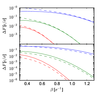
Figure 2: Real space error in the forces measured and estimated with equation 20 for (top) bulk system and (bottom) interfacial system. Measured errors are depicted as solid lines, estimated errors as dashed lines. From top to bottom, the real space cutoff is (blue) $2.0\sigma$, (green) $3.0\sigma$, and (red) $4.0\sigma$. The estimate works well for the bulk system, but fails for the interfacial system.

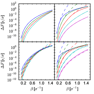
Figure 3: Measured and estimated reciprocal space errors. for (top) a bulk system and (bottom) an interfacial system. The graphs on the left show increasing interpolation order from $P=3$ at the top to $P=6$ at the bottom, with a fixed grid containing 32 grid points in each direction. The graphs on the right show grid density increasing from $2^{2}$ points in each direction at the top to $2^{6}$ points at the bottom, for fixed interpolation order $P=5$. Measured errors are depicted as solid lines. Errors estimated with equations 21 and 24 are depicted as dashed lines, those estimated with equations 21 and III.2 are depicted as dotted lines.

The results of the real space error estimate are given in Figure 2. Results for the reciprocal space error estimates are shown in Figure 3. Except for small values of $\beta$, the real space error estimate works well for the bulk system. In contrast, the error is underestimated in surface simulations. For bulk phase systems, the reciprocal space error estimate with equations 21 and III.2 provides very good results. The approximation with equation 24 strongly overestimates the reciprocal space error when the assumption that $h\beta$ is small is violated. For the interfacial system, the error estimates underpredict the simulation error. Yet, as can be seen from these figures and from Figure 6, the error estimates can be useful for determining the value of the Ewald parameter for which the accuracies in real and reciprocal space are equal, if this information is needed.

The results shown above demonstrate that the error estimates presented here should only be applied to homogeneous bulk systems. Additionally, it should be noted that the error estimate for the real space contribution assumes that the errors in the forces partly cancel. This cancellation of errors cannot occur for the real space contribution to either energy or pressure. This can be easily seen from the following example: Consider three equal, collinear particles, with particle 2 equidistant between particles 1 and 3. The distance between particle 2 and the other particles is larger than the chosen real-space cutoff, so that none of the real-space forces, energies, or pressures are calculated. If the chosen cutoff radius were larger, so that the interactions should be calculated, the force on particle 2 would be zero, because the contributions from particles 1 and 3 cancel. The energy and the pressure that are exerted on particle 2, however, do not cancel but instead are additive. The reason for this behavior is that dispersion interactions, unlike Coulomb interactions, are always attractive. Contributions to the energy thus always have the same sign. As the distance vectors and force vectors for pairwise interactions always point in opposite directions, the contributions to the diagonal components of the virial tensor always have the same sign, too. This in turn means that pressures and energies can be underestimated, even when forces are calculated accurately.

Thus, usage of the above error estimates to set the Ewald and grid parameters is only recommended for bulk systems in which neither the energy nor the pressure is relevant, such as in simulations for determining diffusivities. We show how to determine parameters for interfacial simulations in Section VI.

IV Scaling of the algorithm

The main benefit of mesh-based Ewald methods over traditional Ewald sums is the improved scaling behavior of the mesh-based approach. To examine the scalability of the implemented solver, we have performed simulations with $2^{n}\times 10^{3}$ LJ particles, where $n=0,1,\ldots,10$, with the dispersion PPPM solver and the Ewald summation. The density was $3.64\sigma^{-3}$ in all simulations. The boxes were always cubic. An energy minimization and equilibration over 50 000 timesteps in the $NVT$ ensemble at a reduced temperature $T^{*}=0.85$ was followed by a simulation over 1 000 timesteps in the $NVE$ ensemble. The simulation time of the last 1 000 timesteps was used to measure the performance. These simulations were executed on a single core of an Intel Harpertown E5454 processor with eight 3.0 GHz Xeon cores.

Automated parameter generation was applied in simulations with the Ewald sum.in ’t Veld, Ismail, and Grest (2007) The mesh parameters for the PPPM were set using the error estimate presented in the previous section in the following way. The real space cutoff was chosen as 3.0 $\sigma$. The real space error estimate was then used to set the Ewald parameter to obtain a desired accuracy of 0.01 $\epsilon/\sigma$ in the calculated real space forces. The interpolation order was set to $P=5$. Using these data, the grid spacing was chosen in a way that the accuracy of the reciprocal space forces was smaller then 0.01 $\epsilon/\sigma$ by using equation 24. As the conditions for the validity of the error estimates are fulfilled for the chosen simulations, the comparison we draw here is for different system sizes run with the same accuracy.

As can be seen from Figure 4, which shows the computation time per timestep, the dispersion PPPM approaches the expected scaling behavior of $\mathcal{O}(N\log N)$ with increasing numbers of particles. Its performance becomes several magnitudes faster than the traditional Ewald sum and is thus far more suitable for large-scale simulations. The comparison between the different solvers drawn here should be considered qualitative, as we did not examine whether the two different solvers were run with the same accuracy.

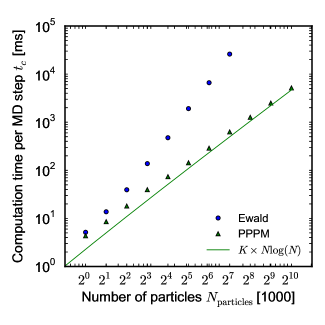
Figure 4: Scaling of the Ewald sum and the PPPM method for dispersion interactions

V Determination of surface tensions from MD simulation

As the need for incorporating long-range dispersion is especially acute for interfacial systems, we have run simulations with explicit interfaces on LJ particles, SPC/E water, and hexane to test the efficiency and accuracy of the dispersion PPPM algorithm. This section briefly summarizes the method applied to simulate surface tensions. Surface tensions can be obtained from MD simulations via two-phase simulations. We use the approach, developed by TolmanTolman (1948) and Kirkwood and Buff,Kirkwood and Buff (1949) in which the surface tension is expressed via

$$\gamma_{p}=\frac{1}{2}\int_{-\infty}^{\infty}\left(p_{\perp}(z)-p_{\parallel}(z)\right)\mathrm{d}z,$$ (27)

where $p_{\perp}(z)=p_{z}(z)$ is the pressure component normal to the surface and $p_{\parallel}(z)=(p_{x}(z)+p_{y}(z))/2$ is the pressure component parallel to the surface. Replacing the integral with an ensemble average leads to

$$\gamma_{p}=\frac{L_{z}}{2}\left(p_{\perp}-p_{\parallel}\right)=\frac{L_{z}}{2}\left[\left\langle p_{z}\right\rangle-\frac{\left\langle p_{x}\right\rangle+\left\langle p_{y}\right\rangle}{2}\right],$$ (28)

where $L_{z}$ is the box dimension in the $z$-direction. The outer factor of $1/2$ takes into account that the simulated system contains two interfaces.

If a cutoff is introduced for the pair potential, the surface tensions calculated with Equation 28 will underestimate the correct surface tension of the simulated material. This error can be estimated by adding a “tail correction” $\gamma_{\mathrm{tail}}$ to the simulated surface tension to provide a better estimate of the correct surface tension

$$\gamma\approx\gamma_{p}+\gamma_{\mathrm{tail}}$$ (29)

from the simulation. The correction can be calculated asChapela, Saville, and Thompson (1977); Blokhuis et al. (1995)

$$\gamma_{\mathrm{tail}} = \frac{\pi}{2}\int_{-\infty}^{\infty}\int_{-1}^{1}\int_{r_{c}}^{\infty}r^{3}\frac{\mathrm{d}U(r)}{\mathrm{d}r}g(r)(1-3s^{2})$$ (30)

$$\times\left(\rho(z)\rho(z-sr)-\left(\rho_{\mathrm{G}}(z)\right)^{2}\right)\mathrm{d}r\mathrm{d}s\mathrm{d}z,$$

where $U(r)$ is the pair potential, $g(r)$ is the radial distribution function, $\rho(z)$ is the simulated density profile, $r_{c}$ is the cutoff radius for the pair potential, and $\rho_{\mathrm{G}}(z)$ is the Gibbs dividing surface

$$\rho_{\mathrm{G}}(z)=\rho_{c}+\frac{\Delta\rho}{2}\mathrm{sgn}(z),$$ (31)

where $\rho_{c}$ is the mean and $\Delta\rho$ is the difference of the densities of the coexisting phases. $g(r)$ was assumed to be unity beyond the cutoff in the calculations of the tail correction. The values for $\rho_{c}$ and $\Delta\rho$, which were also used to calculate the liquid and vapor densities in this study, were obtained from fitting an error function to the simulated density profile.Huang and Webb (1969); Beysens and Robert (1987); Sides, Grest, and Lacasse (1999)

VI Influence of the Ewald and grid parameters on physical properties

The parameters used by the dispersion PPPM have a strong influence on both the efficiency and the accuracy of the simulations. As the presented error estimates fail to describe systems with interfaces, we have run test simulations to determine a set of parameters that can provide both accurate results and acceptable performance for interfacial simulations. These parameters were determined for Lennard-Jones particles and hexane, a nonpolar fluid whose intermolecular interactions are dominated by dispersion. Hexane was modeled using the OPLS-AAJorgensen, Maxwell, and Tirado-Rives (1996) force field.

Simulations with hexane contained 689 hexane molecules that were placed using PackmolMartínez et al. (2009) in a subvolume around the center of the box with volume $50\times 50\times 150$ ų. After an energy minimization with a soft potential and several runs with restricted movement of the particles, the simulations were equilibrated for 1 000 000 timesteps with a timestep of $\Delta t=1$ fs. The temperature was set to $T=300$ K using a Nosé-HooverShinoda, Shiga, and Mikami (2004) thermostat with a damping factor of 0.1 ps. A PPPMHockney and Eastwood (1988) with a real space cutoff of $r_{c}=10$ Å, an Ewald parameter of $\beta=0.17$ Å^-1 and fifth-order interpolation ($P=5$) was used to calculate the electrostatic potential. The grid dimension was set to $20\times 20\times 45$.

The parameters of the PPPM for dispersion are the real space cutoff, the Ewald parameter, the interpolation order, and the grid spacing in each dimension. The influence of the different parameters is already described at the beginning of Section III. Instead of exploring this six-dimensional parameter space, we set the interpolation order to $P=5$ and the real space cutoff $r_{c}=10.0$ Å for the hexane system. This choice of parameters was made because these values are commonly used in MD simulations, although they are in principle arbitrary. We do not claim that these are the optimal choices. For example, using the long-range dispersion solver allows experimenting with smaller values for the real space cutoff and might in this way improve the performance of the calculations. Furthermore, the grid spacing was equal in all three dimensions in the simulations described below, as near cubic grids usually provide most accuracte calculations.

This reduction of the parameter space allows for determining suitable simulation parameters with less effort, but permits reaching a wide range of accuracy in either real or reciprocal space. As the real space cutoff is fixed, the real space accuracy depends only on the Ewald parameter, which is therefore used in the following simulations to tune the real space accuracy. In principle, we could also have fixed the Ewald parameter beforehand and modified the real-space cutoff in our simultations to tune the real-space accuracy, but we decided against it to have better control over the real space calculation time. For a given Ewald parameter and the other parameters fixed, the grid spacing can be altered to tune the reciprocal space accuracy, even though the reachable reciprocal-space accuracy is not unlimited for a fixed Ewald parameter.

We performed surface tension calculations with different settings for the two remaining parameters, the Ewald parameter and the uniform grid spacing. We examined the resulting surface tensions and liquid densities. In addition we determined the rms error in the total forces as well as the real and reciprocal space contributions to the error by comparing the forces calculated for a single snapshot of an equilibrated systems to forces that were calculated using a large real-space cutoff and a very small grid spacing.

Figure 5: Surface tension and density of hexane as a function of the total error in the calculated forces. The arrows point in the direction of increasing Ewald parameter.

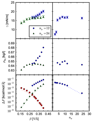
Figure 6: Surface tension, density, and errors in the forces in simulations of hexane. In the lower left graph, the red squares correspond to the real space error, while the triangles and circles correspond to the reciprocal space error when using the fine grid and coarse grids, respectively. The circles in the lower right graph correspond to the reciprocal space error. The Ewald parameter is $\beta=0.28$ Å^-1 in all figures on the right side. Dotted lines are error estimates calculated with Equations 20, 21, and III.2.

The results for the surface tension and density of hexane are given as a function of the total rms error in the forces in Figure 5. In simulations with fewer grid points, the total error is always dominated by the reciprocal space error. In simulations with smaller grid spacings, where the number of grid points in the $x$-direction $n_{x}=24$, the real and reciprocal space error are approximately equal for the highest achieved total accuracy at $\beta=0.28$ Å^-1. As can be seen from Figure 6, the real space error dominates for smaller values of the Ewald parameter $\beta$, whereas the reciprocal space error dominates for larger values of $\beta$.

As the total error decreases, the simulated surface tensions and densities plateau, indicating that further increases in accuracy, which can be obtained by using even finer grids and larger values for the Ewald parameter, will offer little benefit in the accuracy of the measured quantities. Decreasing the Ewald parameter, thereby increasing the real space error, strongly influences the simulated quantities. In contrast, increasing the Ewald parameter and in this way increasing the reciprocal space error has less influence on the results. Physical data begin to change for reciprocal space errors above approximately 0.01 kcal mol^-1 Å^-1. For the examined quantities, the real space error has a stronger influence on the results than the reciprocal space error. The reason for this observation is that an increasing real space error leads to increasing underprediction of the cohesion of a simulated system. For simulations of quantities in which the cohesion does not influence the reults, the influence of the real and reciprocal space error will possibly be different.

The data given in Figure 5 are also given on the left side of Figure 6 as a function of the Ewald parameter. These results, in combination with those from Figure 5, show that an Ewald parameter of approximately $\beta=0.28$ Å^-1 in combination with a real space cutoff $r_{c}=10$ Å provides a sufficient real space accuracy for the performed simulations.

As the results from Figure 5 indicate that increasing the reciprocal space error does not alter the obtained physical data strongly, we have performed further simulations with fixed Ewald parameter with varying grid spacings. Results of these simulations are given on the right side of Figure 6. Increasing the number of grid points $n_{x}$ in the $x$-direction beyond 12 does not alter either the simulated density or surface tensions, although the error in the forces continues to decrease. However, the extended running times required for the finer meshes make these higher fidelity calculations computationally undesirable.

Therefore, we choose $\beta=0.28$ Å^-1 and the grid spacing $h\approx 4.17$ Å as these parameters provide sufficient accuracy. Examining the influence of the parameters of the LJ system provided similar results as those described above. The parameters we obtain for the LJ system are $\beta=1.1\sigma^{-1}$ and $h\approx 1.22\sigma$ for Interpolation order $P=5$ and a real space cutoff of $r_{c}=3\sigma$. The corresponding simulations and results are described in the supporting information support .

VII Application of the solver

To compare our algorithms to existing implementations—a plain cutoff or the Ewald sumin ’t Veld, Ismail, and Grest (2007)—we have performed simulations with systems of LJ particles, SPC/E water,Berendsen, Grigera, and Straatsma (1987) and hexane modeled with the OPLS all-atom force field.Jorgensen, Maxwell, and Tirado-Rives (1996) These systems cover a model system as well as realistic systems in which Coulomb interactions (water) and dispersion interactions (hexane) dominate. Furthermore, these systems have already been studied and allow comparison to results from the literature.in ’t Veld, Ismail, and Grest (2007); Ismail et al. (2007); Chen and Smith (2007); Wang and Zeng (2009); Sakamaki et al. (2011) A comparison with results from Shi et al.Shi, Sinha, and Dhir (2006) is of special interest, as they have also used a PPPM dispersion method to determine the surface tension of SPC/E water.

VII.1 Lennard-Jones particles

The Lennard-Jones simulations were performed in a box with volume $11.01\times 11.01\times 176.16\sigma^{3}$ and 4000 particles that were placed randomly in a subvolume at the center of the box. After minimization using a soft potential, the system was equilibrated for 100 000 timesteps. The timestep was set to 0.005 $\tau$, where $\tau=\sigma\sqrt{m/\epsilon}$. Simulations were executed at reduced temperatures $T^{*}=k_{\mathrm{B}}T/\epsilon\in\{0.7,0.85,1.1,1.2\}$ using a Nosé-HooverShinoda, Shiga, and Mikami (2004) thermostat with damping factor 10 $\tau$. The equations of motion were solved using a velocity Verlet algorithm.Tuckermann et al. (2006) Afterwards, simulations were run for another 1 000 000 timesteps with the same conditions. During that time, instantaneous surface tensions were calculated every timestep. Configurations were stored every 1 000 timesteps to calculate the density profile. For simulations without a long-range dispersion solver, we examined cutoffs of $2.5\sigma$, $5\sigma$, and $7.5\sigma$. Simulations with an Ewald solver were performed with cutoffs of $3\sigma$, $4\sigma$, and $5\sigma$. We relied on automatic generation of the Ewald parameter and the cutoff for the $\mathbf{k}$ vectors. We used the value of 0.05 as the desired relative accuracy in the forces.in ’t Veld, Ismail, and Grest (2007) The resulting Ewald parameters were $0.60\sigma^{-1}$, $0.45\sigma^{-1}$, and $0.36\sigma^{-1}$; the number of $\mathbf{k}$ vectors were 1616, 677, and 320 for the different cutoffs. In simulations with the dispersion PPPM we used cutoffs of $3\sigma$, $4\sigma$, and $5\sigma$. We used $P=5$, $\beta=1.1\sigma^{-1}$ and a grid with $9\times 9\times 144$ mesh points in agreement with our results from Section VI.

Table 2: Results of the validation runs for the LJ particles. Uncertainties given in parentheses

				Surface tension, $\epsilon\sigma^{-2}$
$T^{*}$	solver	$r_{c}$ ($\sigma$)	$\rho_{\mathrm{liq}}$ ($\sigma{-3}$)	$\gamma_{p}$	$\gamma_{t}$	$\gamma$	$t_{c}$ (ms)
0.7	cutoff	2.5	0.7865	0.588(30)	0.327	0.915(30)	3.7
		5.0	0.8349	1.006(30)	0.125	1.131(30)	24.8
		7.5	0.8390	1.112(30)	0.057	1.169(30)	80.2
	Ewald	3.0	0.8332	1.085(30)	-	1.085(30)	123.2
		4.0	0.8371	1.121(30)	-	1.121(30)	77.5
		5.0	0.8393	1.134(30)	-	1.134(30)	87.63
	PPPM	3.0	0.8404	1.158(30)	-	1.158(30)	19.59
		4.0	0.8407	1.167(30)	-	1.167(30)	32.83
		5.0	0.8408	1.157(30)	-	1.157(30)	52.67
0.85	cutoff	2.5	0.6996	0.341(22)	0.221	0.562(22)	3.1
		5.0	0.7672	0.700(26)	0.098	0.798(26)	22.6
		7.5	0.7730	0.781(32)	0.046	0.827(32)	73.2
	Ewald	3.0	0.7651	0.742(24)	-	0.742(24)	122.2
		4.0	0.7706	0.799(26)	-	0.799(26)	75.0
		5.0	0.7732	0.803(28)	-	0.803(28)	76.0
	PPPM	3.0	0.7748	0.817(26)	-	0.817(26)	18.81
		4.0	0.7758	0.829(24)	-	0.829(24)	30.00
		5.0	0.7756	0.829(28)	-	0.829(28)	48.24
1.1	cutoff	2.5	n.a.	0.023(26)	n.a.	0.023(26)	1.4
		5.0	0.6282	0.278(26)	0.042	0.320(26)	15.5
		7.5	0.6385	0.293(24)	0.026	0.319(24)	50.7
	Ewald	3.0	0.6243	0.270(26)	-	0.270(26)	118.2
		4.0	0.6354	0.293(24)	-	0.293(24)	68.4
		5.0	0.6452	0.315(26)	-	0.315(26)	56.2
	PPPM	3.0	0.6451	0.314(24)	-	0.314(24)	15.69
		4.0	0.6448	0.330(26)	-	0.330(26)	23.57
		5.0	0.6462	0.302(22)	-	0.302(22)	37.19
1.2	cutoff	2.5	n.a.	0.001(20)	n.a.	0.001(20)	1.4
		5.0	0.5613	0.113(20)	0.025	0.138(20)	11.8
		7.5	0.5725	0.159(26)	0.013	0.172(26)	38.8
	Ewald	3.0	0.5497	0.128(24)	-	0.128(24)	118.9
		4.0	0.5647	0.141(26)	-	0.141(26)	65.4
		5.0	0.5728	0.159(24)	-	0.159(24)	49.9
	PPPM	3.0	0.5767	0.164(24)	-	0.164(24)	13.73
		4.0	0.5757	0.155(22)	-	0.155(22)	21.10
		5.0	0.5766	0.154(26)	-	0.154(26)	32.24

Results are given in Table 2. Overall, we find good agreement with results from the literature.in ’t Veld, Ismail, and Grest (2007); Wang and Zeng (2009) The simulated densities and surface tensions show a strong dependence on the chosen cutoff in simulation without a long-range dispersion solver. For simulations at higher temperatures, systems with small cutoffs were so close to the critical point that error functions were no longer appropriate for describing the density profile, as can be seen from Figure 7. Agreement between simulated data with and without long-range dispersion solver can only be obtained when using a large cutoff in simulations without the long-range solver.

Unlike the simulations with a long-range cutoff, the results for the dispersion PPPM method do not show a dependence on the switching radius. For the Ewald sum, a slight dependence of the physical data remains, which we attribute to the automated parameter generation routine in combination with the specified accuracy.

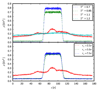
Figure 7: Measured density profiles for simulations of LJ particles: (top) simulations with cutoff $r_{c}=2.5\sigma$ and (bottom) simulations at a reduced temperature of $T^{*}=1.1$.

VII.2 SPC/E water

Simulations with SPC/E water were performed with 5 000 water molecules in a box of $50\times 50\times 150$ ų. The initial configurations of the particles were created using Packmol.Martínez et al. (2009) If not explicitly given in the following, the simulation settings were as those for hexane described in Section VI.

Simulations were executed at 300, 350, and 400 K. For each solver, we used cutoffs of 10, 12, and 16 Å for the sum in real space for dispersion and Coulomb interaction. The SHAKE algorithmRyckaert, Berendsen, and Ciscotti (1977) was used to constrain the bond lengths and bond angles.

A PPPMHockney and Eastwood (1988) solver was used for long-range electrostatics in simulations with a plain cutoff for dispersion interaction. We picked interpolation order $P=5$ and a grid of $24\times 24\times 54$ mesh points as grid parameters. The Ewald parameter was $\beta$ = 0.255, 0.226, and 0.184 Å^-1 for the three different cutoffs. In simulations with the traditional Ewald sum for dispersion and Coulomb interactions, the Ewald parameter and number of $\mathbf{k}$ vectors were generated for a desired relative accuracy of 0.05. The Ewald parameters were set to approximately 0.18, 0.15, and 0.11 Å^-1 and the number of $\mathbf{k}$ vectors were 748, 436, and 183 for the different cutoffs. In simulations with a PPPM solver for dispersion, we used interpolation order $P=5$. Following our results from Section VI, a grid with $12\times 12\times 36$ mesh points was used for the dispersion interactions. The Ewald parameter for dispersion was set to $\beta$ = 0.28 Å^-1 for all cutoffs. The parameters used for the long-range solver for the Coulomb interaction were the same as those in simulations with a plain cutoff for dispersion.

Table 3: Results of the validation runs for the SPC/E water. Simulation marked with a dagger was run with higher precision.

				Surface tension, mN/m
$T$ (K)	solver	$r_{c}$ (Å)	$\rho_{\mathrm{liq}}$ (kg/L)	$\gamma_{p}$	$\gamma_{t}$	$\gamma$	$t_{c}$ (ms)
300	cutoff	10.0	0.9882	54.59(100)	5.27	59.86(100)	169
		12.0	0.9918	56.38(100)	3.72	60.10(100)	259
		16.0	0.9944	57.51(84)	2.12	59.63(84)	531
	Ewald	10.0	0.9964	59.39(100)	-	59.39(100)	455
		12.0	0.9962	60.84(100)	-	60.84(100)	474
		16.0	0.9967	60.56(100)	-	60.56(100)	756
	PPPM	10.0	0.9965	60.72(90)	-	60.72(90)	229
		12.0	0.9964	60.11(80)	-	60.11(80)	364
		16.0	0.9963	59.64(90)	-	59.64(90)	737
		10.0	0.9964	61.06(80)	-	61.06(80) †	-
350	cutoff	10.0	0.9539	47.40(60)	4.81	52.21(60)	166
		12.0	0.9576	48.71(60)	3.42	52.13(60)	254
		16.0	0.9607	49.78(70)	1.96	51.74(70)	517
	Ewald	10.0	0.9617	52.55(80)	-	52.55(80)	448
		12.0	0.9622	51.72(70)	-	51.72(70)	531
		16.0	0.9626	52.13(70)	-	52.13(70)	743
	PPPM	10.0	0.9629	53.29(60)	-	53.29(60)	239
		12.0	0.9631	52.35(70)	-	52.35(70)	350
		16.0	0.9630	52.30(70)	-	52.30(70)	737
400	cutoff	10.0	0.9067	39.89(60)	4.20	44.09(60)	165
		12.0	0.9114	40.42(60)	3.02	43.44(60)	244
		16.0	0.9151	41.36(58)	1.75	43.11(58)	494
	Ewald	10.0	0.9164	42.97(60)	-	42.97(60)	438
		12.0	0.9168	43.71(70)	-	43.71(70)	512
		16.0	0.9172	43.34(60)	-	43.34(60)	716
	PPPM	10.0	0.9177	43.98(60)	-	43.98(60)	240
		12.0	0.9178	43.89(60)	-	43.89(60)	345
		16.0	0.9178	43.44(60)	-	43.44(60)	710

Table 3 shows the results of the simulations. When not using a long range solver, the simulated density shows slight dependence on the chosen cutoff radius, whereas practically no dependence can be observed when using a long-range solver for dispersion. For simulated surface tensions, neither the cutoff nor the chosen dispersion solver have a strong influence. The weak or non-existent influence on physical properties of the way dispersion interactions are calculated is due to the fact that Coulomb, and not dispersion, interactions are the dominant contribution to the interactions in this system.

Again, our results are in good agreement with the majority of the literature; in ’t Veld, Ismail, and Grest (2007); Chen and Smith (2007); Wang and Zeng (2009); Sakamaki et al. (2011) however, they differ substantially from those reported by Shi et al.Shi, Sinha, and Dhir (2006), who performed simulations of SPC/E with a PPPM for dispersion, too. For example, their result for the surface tension at 300 K is more than 70 mN/m (read from Fig. 6 in Ref. Shi, Sinha, and Dhir, 2006), whereas the surface tensions in our simulations are always about 60 mN/m, consistent with other studies. To ensure the validity of our results we have run an additional simulation with increased accuracy, in which we set the Ewald parameter for dispersion to $\beta=0.3$ Å^-1, the interpolation order to $P=5$ and the grid spacing to $h\approx 1.56$ Å corresponding to $32\times 32\times 96$ mesh points. Results of this simulation, marked with a dagger in Table 3, are in good agreement with the rest of our results. The increased value for the surface tension in simulations by Shi et al. might be related to the small number of water molecules (800) in their simulation or the choice of the Ewald parameter (0.9, units not given), but is most likely caused by their short sampling time of only 100 000 timesteps, as substantially longer run times are required to achieve equilibration for water at an interface.Ismail, Grest, and Stevens (2006)

VII.3 Hexane

If not given in the following, all settings for the hexane simulations were as those reported in Section VI. We studied temperatures of 300, 350, and 400 K and cutoffs of 10, 12, and 16 Å.

In simulations with a plain cutoff for dispersion, a PPPM solver was used for electrostatics. The grid dimension was set to $20\times 20\times 45$ and the interpolation order to $P=5$. The Ewald parameter was approximately $\beta$ = 0.17, 0.16, and 0.14 Å^-1 for the different cutoffs. The desired precision was set to 0.05 in simulations with the Ewald method for dispersion and Coulomb interactions. The resulting Ewald parameters and number of $\mathbf{k}$ vectors were the same as those in simulations with SPC/E water. In simulations with the PPPM for dispersion, the interpolation order was set to $P=5$, the grid size was set to $12\times 12\times 36$ and the Ewald parameter was set to $\beta$ = 0.28 Å^-1 in all simulations. Coulomb interactions were treated in a same way as in simulations with a cutoff for dispersion.

Table 4: Results of the validation runs for the OPLS hexane

				Surface tension, mN/m
$T$ (K)	solver	$r_{c}$ (Å)	$\rho_{\mathrm{liq}}$ (kg/L)	$\gamma_{p}$	$\gamma_{t}$	$\gamma$	$t_{c}$ (ms)
300	cutoff	10.0	0.6058	7.83(50)	4.59	12.42(50)	137
		12.0	0.6251	10.21(50)	3.75	13.96(50)	207
		16.0	0.6367	13.00(50)	2.34	15.34(50)	421
	Ewald	10.0	0.6368	14.40(50)	-	14.40(50)	409
		12.0	0.6385	14.91(50)	-	14.91(50)	414
		16.0	0.6410	14.91(56)	-	14.91(56)	634
	PPPM	10.0	0.6434	16.41(50)	-	16.41(50)	201
		12.0	0.6439	16.16(50)	-	16.16(50)	352
		16.0	0.6453	15.89(50)	-	15.89(50)	601
350	cutoff	10.0	0.5237	2.18(40)	2.13	4.31(40)	118
		12.0	0.5534	4.78(40)	2.20	6.98(40)	182
		16.0	0.5721	7.44(50)	1.71	9.15(50)	383
	Ewald	10.0	0.5722	8.09(50)	-	8.09(50)	384
		12.0	0.5778	8.52(40)	-	8.52(40)	438
		16.0	0.5805	9.03(40)	-	9.03(40)	575
	PPPM	10.0	0.5823	9.97(44)	-	9.97(44)	183
		12.0	0.5839	9.77(60)	-	9.77(60)	276
		16.0	0.5851	9.89(44)	-	9.89(44)	547
400	cutoff	10.0	n.a	-1.55(32)	n.a.	-1.55(32)	92
		12.0	0.4467	0.30(36)	0.74	1.04(36)	149
		16.0	0.4905	1.83(36)	0.85	2.68(36)	316
	Ewald	10.0	0.4881	2.26(50)	-	2.26(50)	368
		12.0	0.5037	3.07(32)	-	3.07(16)	402
		16.0	0.5039	3.43(40)	-	3.43(40)	498
	PPPM	10.0	0.5099	4.59(36)	-	4.59(36)	158
		12.0	0.5106	4.66(40)	-	4.66(40)	234
		16.0	0.5157	4.45(46)	-	4.45(46)	452

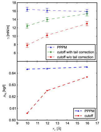
Figure 8: Surface tensions and densities simulated when using a PPPM or a plain cutoff for dispersion. Results obtained when not using a long-range solver strongly depend on the chosen cutoff and approach the results of the simulation with the PPPM with increasing cutoff size.

The results are summarized in Table 4. The chosen cutoff radius has a strong influence on the results in simulations without a long-range dispersion solver. In contrast, the results for Ewald summation show weak and the results for the PPPM show no dependence on the chosen cutoff radius. Our results for the PPPM are in good agreement with those from Ismail et al.Ismail et al. (2007) in simulations with an Ewald sum for dispersion. This, and the fact that the chosen cutoff does not influence the results, confirms the validity of our simulations and the good choice of the Ewald and grid parameters. Our simulations with Ewald sums provide lower surface tensions, which is caused by insufficient accuracy in these simulations. As can be seen from Figure 8, the simulation results when not using a long-range dispersion solver approach those obtained with the PPPM when increasing the cutoff. However, even those with a cutoff of 16 Å provide surface tensions and densities that are below those obtained from PPPM simulations.

VIII Performance Comparison

To measure the simulation time, each of the simulations in Section VII was run for 1 000 timesteps on a single core. The resulting computation times per timestep $t_{c}$ are given in the last column of Tables 2 to 4. The simulations were executed on Intel Harpertown E5454 processors with eight 3.0 GHz Xeon cores.

For a fair comparison between the different solvers, one should consider different solvers at the same temperature with the cutoff that provides the results that are obtained in the limit of high accuracy simulations. If for a given solver and temperatures different cutoffs provided accurate results, the fastest of those simulations should be used.

A quick comparison of the PPPM with the Ewald shows that simulations with the PPPM were faster in all cases. As the Ewald sum was always slower than the PPPM, we omit comparisons between the Ewald solver and the plain cutoff and continue with comparing simulations with a PPPM to those with a plain cutoff. For the LJ system, accurate surface tensions and densities were obtained only in simulation in which the cutoff was $r_{c}=7.5\sigma$ in simulations without long-range dispersion solvers. For simulations with the PPPM for dispersion $r_{c}=3\sigma$ provides proper results with maximum efficiency. Comparing the corresponding simulation times shows the computational superiority of using the PPPM for dispersion.

In simulations with water, the results of the comparison are different when examining the simulated surface tensions or simulated densities. As surface tensions were approximately the same throughout all simulations, the PPPM was outperformed by the plain cutoff for this comparison. The reason for the observed behavior is not the choice of parameters, but the dominance of Coulomb interaction in the examined system. When comparing the simulation times it has to be kept in mind that the simulations with a plain cutoff are incorrect during the simulations and are only corrected a posteriori. If this correction is not possible after the simulations, or if a correct value of the surface tension is required during the simulations for any reason, a larger cutoff is required in simulations with a plain cutoff. Simulations with a PPPM are more efficient in such cases. The increase in simulation time is about 35 percent when using the PPPM for dispersion compared to a plain cutoff.

If highly accurate simulated densities are important, then the cutoff for dispersion interactions should be chosen to be at least $r_{c}=12$ Å in simulations without long-range dispersion solvers. Comparing the simulation time of these simulations to those with a PPPM with a cutoff $r_{c}=10$ Å shows that using the PPPM is computationally favorable in this case.

For simulations of hexane, in which dispersion interactions dominate, the largest cutoff has to be selected in simulations without long-range dispersion solvers, whereas a small cutoff is sufficient in simulations with the PPPM. As a consequence, the simulations with the PPPM were much faster than those without a long-range dispersion solver.

We would like to note that simulations with the long-range dispersion solver were run without tabulating the pair potential. Including this tabulation will results in additional speed-up of the simulations and might change the comparison above.

IX Conclusions and Outlook

We present a PPPM algorithm for dispersion interactions that calculates long-range dispersion forces accurately and efficiently for inhomogeneous systems. When used correctly, this solver strongly reduces the error that is caused when truncating the pair potential at a plain cutoff and thus provides a better description of the physics of a simulated system.

We derived and tested error estimates that describe the effect of the parameters of the PPPM on simulation results. The presented error estimates are only valid for bulk phase systems and should not be relied on when simulated energies or pressures are relevant.

For not having to rely on the presented error measures, we explored the parameter space to provide parameters that can be used in future simulations. For real physical systems of surfaces, a combination of the Ewald parameter $\beta=0.28$ Å^-1, the interpolation order $P=5$, the grid spacing $h\approx 4.17$ Å, and the real space cutoff $r_{c}=10.0$ Å provided good results for different materials at different temperatures.

We have applied the developed algorithm to study the surface tension of LJ particles, SPC/E water, and hexane. The described algorithm outperforms Ewald summation for all systems that were examined in this study in terms of simulation time.

Comparing the PPPM to simulations with a plain cutoff show that the PPPM is favorable when correction methods cannot be applied or correction methods do not work properly, as for example near the critical point or in some of our hexane and LJ simulations. In systems that are dominated by dispersion, the PPPM outperforms simulations without long-range solvers in tems of computation time, as latter simulations require larger cutoffs.

For strongly charged systems, the PPPM provides a benefit in simulation time only if densities are needed at a high accuracy. In other cases a plain cutoff is favorable in terms of computation time here. However, the advantage of correctness during the simulation and the applicability to arbitrarily shaped surfaces remains.