Recent theoretical improvement of hadronic $B_{(s)}$ decays

Abstract

In this mini-review, we show that a lot of theoretical efforts have been made for the theoretical study of two body hadronic $B_{(s)}$ and $B_{c}$ decays. In addition to many next-to-leading order or even next-to-next-to leading order $\alpha_{s}$ corrections made, we also study many of the previously unknown next-to-leading order power corrections. While the former corrections are theoretically solid, the latter corrections are phenomenologically more important. In the QCD factorization approach based on collinear factorization, there is difficulty to deal with the power correction diagrams due to the endpoint singularity. Thus many of these analysis use phenomenological method. In the perturbative QCD approach based on $k_{T}$ factorization, the endpoint singularity is killed by including the quark transverse momentum. Therefore we can calculate the annihilation type diagrams quantitatively, which give the right sign for the direct CP asymmetry parameters. More and more $B_{(s)}$ decays channels, especially the pure annihilation type decays have been measured by the recent experiments to confirm our theoretical predictions. More channels are predicted for future experiments, such as the charmless and charmed $B_{s}$ and $B_{c}$ hadronic decays and the decays involving a scalar, axial vector, even a tensor meson in the final states.

I Introduction

In the LHC era of particle physics, heavy flavor physics is still one of the hot topics in particle physics. Most of the standard model free parameters belong to the flavor part. One of the four experiments, the LHCb experiment focus mainly on the B physics, although other two experiments-ATLAS and CMS also providing us rich data of B physics. In fact, while the two B factories continue to analyze data, two new super B factories are preparing for 100 more luminosity. With the big achievements in experiments, the theoretical improvement of B physics has been a little bit slow down.

Although many of the next-to-leading order or even next-to-next-to-leading order $\alpha_{s}$ corrections have been done in the perturbative QCD approach pirho , the QCD factorization approach and the soft-collinear-effective theory studynext , the phenomenologically more important power corrections have not been systematically studied in these approaches. It has been demonstrated that in many non-leptonic B decays, the previously missed power correction, such as annihilation type diagrams are very important in the direct CP asymmetry and polarization study of vector meson final states cheng . As pointed out, these power corrections are not calculable in the QCD factorization approach with endpoint singularity bbns . In fact, the well defined perturbative QCD approach with $k_{T}$ factorization pqcd can calculate all of these kinds of diagrams without ambiguity.

In two body hadronic $B_{(s)}$ decays, the light final state mesons and their constituent quarks inside are collinear objects at the rest frame of $B_{(s)}$ meson. The light spectator quark in the $B_{(s)}$ meson is rather soft. Therefore a hard gluon is needed to transform it into a collinear object. The dominant contribution is perturbative. However, the calculation is sometimes divergent at the endpoint of the meson distribution amplitudes. To deal with this unphysical singularity, one leaves the form factor diagrams to non-perturbative contributions in QCD factorization approach and soft-collinear effective theory (SCET)scet . For the annihilation type diagrams, the QCD factorization approach just parameterizes it as free parameters; while SCET argues it as small power corrections. In fact, the quark carries very little longitudinal momentum at the endpoint, therefore the transverse momentum of quark is no longer negligible. In the perturbative QCD approach, we keep the transverse momentum of quark, which acts as a natural regulator of the endpoint divergence. Including another momentum scale (transverse momentum) in QCD will produce large double logarithms in the perturbative calculations, so that we have to use the renormalization group equation to do the resummation. A Sudakov factor is produced, which suppresses the endpoint contributions to keep the perturbative calculation healthy.

In this paper, we will show that many of the leading order and also next-to-leading order perturbative QCD calculations of $B_{(s)}$ and $B_{c}$ decays have been tested in the experiments and more and more channels are predicted for future experiments. All of the charmless or charmed meson decays of $B_{s}$ meson have been studied some years ago in the perturbative QCD approach bs ; 08031073 and the QCD factorization approach cheng ; bbns . Some of the charmless $B_{s}$ decays are also discussed in the soft-collinear effective theory SCETBs ; scetvp . Recently, a scalar meson, axial vector meson, or tensor meson involved in the final states are also studied. Since the LHC experiment will produce numerous $B_{c}$ mesons, the intensive study of $B_{c}$ meson hadronic decays are also studied, which include the charmless final states, one or two D mesons in the final states and even final states involving scalar or tensor mesons.

II Factorization method in QCD for hadronic $B_{(s)}$ decays

All the hadronic $B_{(s)}$ decays are weak decays. In the quark level, the weak transitions are summarized as effective four quark operators with QCD corrections. The weak effective Hamiltonian $\mathcal{H}_{eff}$ can be written as rmp681125

$$\mathcal{H}_{eff}= \frac{G_{F}}{\sqrt{2}}\left\{\sum_{q=u,c}V_{qb}^{*}V_{qX}\left[C_{1}(\mu)O_{1}^{q}(\mu)+C_{2}(\mu)O_{2}^{q}(\mu)\right]-V_{tb}^{*}V_{tX}\left[\sum_{i=3}^{10}C_{i}(\mu)O_{i}(\mu)\right]\right\},$$ (1)

with $V_{qb(X)}$ and $V_{tb(X)}$ ($X=d,s$) the Cabibbo-Kobayashi-Maskawa (CKM) matrix elements. The current-current (tree) local four-quark operators are:

$$O_{1}^{q}=(\bar{b}_{\alpha}q_{\beta})_{V-A}(\bar{q}_{\beta}X_{\alpha})_{V-A},\;\;\;O_{2}^{q}=(\bar{b}_{\alpha}q_{\alpha})_{V-A}(\bar{q}_{\beta}X_{\beta})_{V-A};$$ (2)

the QCD penguin operators are

$$O_{3}=(\bar{b}_{\alpha}X_{\alpha})_{V-A}\sum_{q^{\prime}}(\bar{q}^{\prime}_{\beta}q^{\prime}_{\beta})_{V-A},\;\;\;O_{4}=(\bar{b}_{\alpha}X_{\beta})_{V-A}\sum_{q^{\prime}}(\bar{q}^{\prime}_{\beta}q^{\prime}_{\alpha})_{V-A},$$ (3)

$$O_{5}=(\bar{b}_{\alpha}X_{\alpha})_{V-A}\sum_{q^{\prime}}(\bar{q}^{\prime}_{\beta}q^{\prime}_{\beta})_{V+A},\;\;\;O_{6}=(\bar{b}_{\alpha}X_{\beta})_{V-A}\sum_{q^{\prime}}(\bar{q}^{\prime}_{\beta}q^{\prime}_{\alpha})_{V+A},$$ (4)

and the electro-weak penguin operators are

$$O_{7}=\frac{3}{2}(\bar{b}_{\alpha}X_{\alpha})_{V-A}\sum_{q^{\prime}}e_{q^{\prime}}(\bar{q}^{\prime}_{\beta}q^{\prime}_{\beta})_{V+A},\;\;O_{8}=\frac{3}{2}(\bar{b}_{\alpha}X_{\beta})_{V-A}\sum_{q^{\prime}}e_{q^{\prime}}(\bar{q}^{\prime}_{\beta}q^{\prime}_{\alpha})_{V+A},$$ (5)

$$O_{9}=\frac{3}{2}(\bar{b}_{\alpha}X_{\alpha})_{V-A}\sum_{q^{\prime}}e_{q^{\prime}}(\bar{q}^{\prime}_{\beta}q^{\prime}_{\beta})_{V-A},\;\;O_{10}=\frac{3}{2}(\bar{b}_{\alpha}X_{\beta})_{V-A}\sum_{q^{\prime}}e_{q^{\prime}}(\bar{q}^{\prime}_{\beta}q^{\prime}_{\alpha})_{V-A},$$ (6)

where $\alpha$ and $\beta$ are the color indices and $q^{\prime}$ are the active quarks at the scale $m_{b}$, i. e. $q^{\prime}=(u,d,s,c,b)$. The left-handed and right-handed currents are defined as $(\bar{b}_{\alpha}q_{\beta})_{V-A}=\bar{b}_{\alpha}\gamma_{\mu}(1-\gamma_{5})q_{\beta}$ and $(\bar{q}^{\prime}_{\beta}q^{\prime}_{\alpha})_{V+A}=\bar{q}^{\prime}_{\beta}\gamma_{\mu}(1+\gamma_{5})q^{\prime}_{\alpha}$, respectively. The Wilson coefficients $C_{i}^{\prime}$s are calculated by the renormalization group equations to include the next-to-leading order QCD corrections.

When doing the hadronic matrix elements calculations, we need to deal with scales around $\sqrt{\Lambda_{QCD}m_{b}}$, which is usually called factorization scale. Scales below this scale are categorized as non-perturbative physics, which is described by form factors or meson wave functions. In the generalized factorization approach prd58094009 , the QCD corrected Wilson coefficients are scale dependent while the matrix elements described by the form factors are scale independent physical quantities. It is later improved by the QCD factorization approach bbns to remove the scale dependence in the decay amplitudes by including the vertex corrections together with the hard scattering diagrams shown at Fig.1(c) and (d). In this collinear factorization based theory, however, there is endpoint singularity at the higher twist calculation and the annihilation type diagrams shown in Fig2. Those annihilation type diagrams are later proved to be important cheng . Similar to the QCD factorization approach, the soft-collinear effective theory scet also leave part of the soft contribution in the form factor diagrams shown in Fig.1(a) and (b) as non-perturbative contribution. This makes the soft-collinear effective theory less predictive, since it requires more free parameters to be determined by experiments SCETBs ; scetvp .

In the perturbative QCD approach, we keep the transverse momentum of quarks to kill the endpoint divergence. Therefore, we have one more scale, i.e. the quark transverse momentum than the QCD factorization approach and SCET. The factorization formula in pQCD approach is then

$$C(t)\otimes H(x,t)\otimes\Phi(x)\otimes\exp[-s(P,b)-2\int^{t}_{1/b}\frac{d\mu}{\mu}\gamma_{q}(\alpha_{s}(\mu))],$$ (7)

where $C(t)$ are the corresponding Wilson coefficients of four quark operators, which include the dynamics of physics larger than $m_{b}$ scale. The Sudakov evolution $\exp[-s(P,b)]$ npb193381 are from the resummation of double logarithms $\ln^{2}(Pb)$, with P denoting the dominant light-cone component of meson momentum. $\gamma_{q}=-\alpha_{s}/\pi$ is the quark anomalous dimension in axial gauge. All non-perturbative components are organized in the form of hadron wave functions $\Phi(x)$, which may be extracted from experimental data or other non-perturbative method, such as QCD sum rules. Since non-perturbative dynamics has been factored out, one can evaluate all possible Feynman diagrams for the six-quark amplitude straightforwardly, which include both factorizable and non-factorizable emission contributions shown in Fig.1. Factorizable and non-factorizable annihilation type diagrams shown in Fig.2 are also calculable without endpoint singularity.

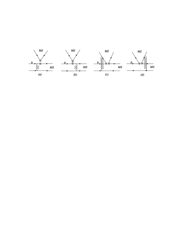
Figure 1: The leading order emission tip Feynman diagrams

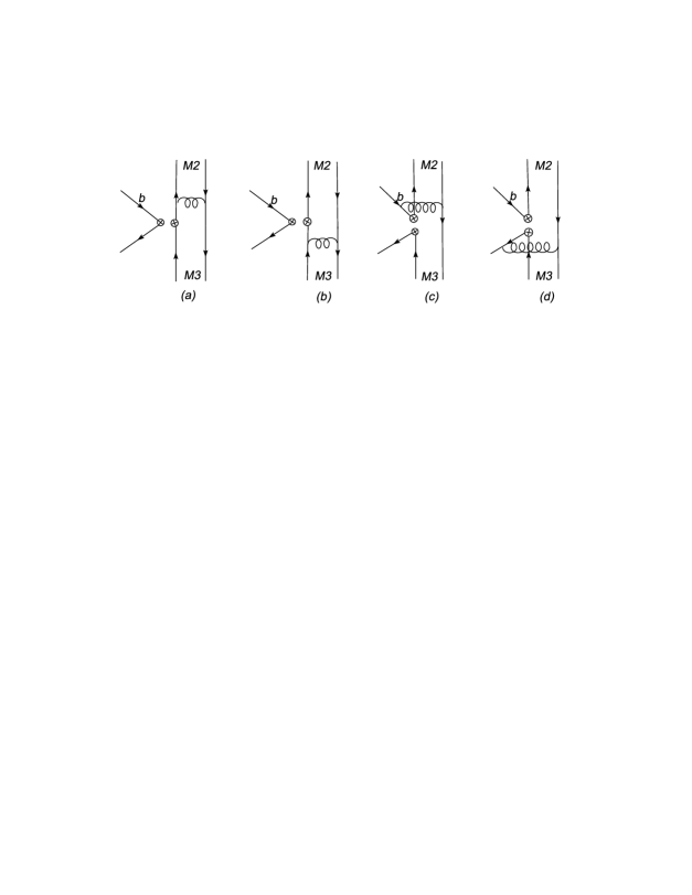
Figure 2: The leading order annihilation type Feynman diagrams

II.1 Wave Functions of the $B_{s}$ Meson

In order to calculate the analytic formulas of the decay amplitudes, we need the light cone wave functions decomposed in terms of the spin structure. In general, the light cone wave functions are decomposed into 16 independent components, $1_{\alpha\beta}$, $\gamma^{\mu}_{\alpha\beta}$, $\sigma^{\mu\nu}_{\alpha\beta}$, $(\gamma^{\mu}\gamma_{5})_{\alpha\beta}$, $\gamma_{5\alpha\beta}$. If the considered meson is the heavy $B$ or $B_{s}$ meson, the $B_{(s)}$ meson light-cone matrix element can be decomposed as grozin ; qiao

$$\int d^{4}ze^{ik_{1}\cdot z}\langle 0|\bar{b}_{\alpha}(0)s_{\beta}(z)|{B_{s}}(P_{B_{s}})\rangle$$ (8)

$$= \frac{i}{\sqrt{6}}\left\{(\not\!P_{B_{s}}+M_{B_{s}})\gamma_{5}\left[\phi_{B_{s}}({k_{1}})-\frac{\not n-\not v}{\sqrt{2}}\bar{\phi}_{B_{s}}({k_{1}})\right]\right\}_{\beta\alpha}.$$

From the above equation, one can see that there are two Lorentz structures in the $B_{s}$ meson distribution amplitudes, that obey the following normalization conditions

$$\int\frac{d^{4}k_{1}}{(2\pi)^{4}}\phi_{B_{s}}({k_{1}})=\frac{f_{B_{s}}}{2\sqrt{6}},~{}~{}~{}\int\frac{d^{4}k_{1}}{(2\pi)^{4}}\bar{\phi}_{B_{s}}({k_{1}})=0.$$ (9)

In general, one should consider these two Lorentz structures in the calculations of $B_{s}$ meson decays. Since the contribution of $\bar{\phi}_{B_{s}}$ is numerically small ly , its contribution can be neglected. With this approximation, we only keep the first term in the square bracket from the full Lorentz structure in Eq. (8)

$$\Phi_{B_{s}}=\frac{i}{\sqrt{6}}(\not\!P_{B_{s}}+M_{B_{s}})\gamma_{5}\phi_{B_{s}}({k_{1}}).$$ (10)

Usually the hard part is always independent of one of the $k_{1}^{+}$ and/or $k_{1}^{-}$. The ${B_{s}}$ meson wave function is then a function of the variables $k_{1}^{-}$ (or $k_{1}^{+}$) and $k_{1}^{\perp}$ only,

$$\phi_{B_{s}}(k_{1}^{-},k_{1}^{\perp})=\int\frac{dk_{1}^{+}}{2\pi}\phi_{B_{s}}(k_{1}^{+},k_{1}^{-},k_{1}^{\perp})~{}.$$ (11)

The $B_{s}$ meson’s wave function in the $b$-space can be expressed by

$$\Phi_{B_{s}}(x,b)=\frac{i}{\sqrt{6}}\left[\not\!P_{B_{s}}\gamma_{5}+M_{B_{s}}\gamma_{5}\right]\phi_{B_{s}}(x,b),$$ (12)

where $b$ is the conjugate space coordinate of the transverse momentum $k^{\perp}$.

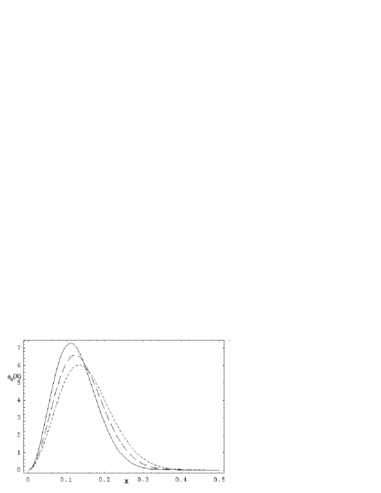
Figure 3: $B_{s}$ meson distribution amplitudes. The solid-, dashed-, and tiny-dashed- lines correspond to $\omega_{B}=0.45~{}\mathrm{GeV}$, $0.5~{}\mathrm{GeV}$, and $0.55~{}\mathrm{GeV}$, respectively.

In this study, we use the model function similar to that of the $B$ meson which is

$$\phi_{B_{s}}(x,b)=N_{B_{s}}x^{2}(1-x)^{2}\exp\left[-\frac{M_{B_{s}}^{2}\ x^{2}}{2\omega_{b}^{2}}-\frac{1}{2}(\omega_{b}b)^{2}\right],$$ (13)

with $N_{B_{s}}$ the normalization factor. In recent years, a lot of studies have been performed for the $B_{d}^{0}$ and $B^{\pm}$ decays in the pQCD approach pqcd . The parameter $\omega_{b}=0.40~{}\mathrm{GeV}$ has been fixed using the rich experimental data on the $B_{d}^{0}$ and $B^{\pm}$ mesons. In the SU(3) limit, this parameter should be the same in $B_{s}$ decays. However, facing the high precision experimental data, one has to consider the small SU(3) breaking effect, i.e. the $s$ quark momentum fraction should be a little larger than that of the $u$ or $d$ quark in the lighter $B$ mesons. The shape of the distribution amplitude is shown in Fig.3 for $\omega_{B}=0.45~{}\mathrm{GeV}$, $0.5~{}\mathrm{GeV}$, and $0.55~{}\mathrm{GeV}$. It is easy to see that the larger $\omega_{b}$ gives a larger momentum fraction to the $s$ quark. We use $\omega_{b}=0.50\pm 0.05~{}\mathrm{GeV}$ in this paper for the $B_{s}$ decays bs .

II.2 $B_{c}$ meson wave function

For $B_{c}$ meson, we only consider the contribution from the first Lorentz structure, like $B_{q}\,(q=u,d,s)$ meson,

$$\Phi_{B_{c}}(x)=\frac{i}{\sqrt{2N_{c}}}(\makebox[-1.5pt][l]{/}P+m_{B_{c}})\gamma_{5}\phi_{B_{c}}(x,b).$$ (14)

Consisting of two heavy quarks (b,c), the $B_{c}$ meson is usually treated as a heavy quarkonium system. In the non-relativistic limit, we adopt the model for the distribution amplitude asbc :

$$\phi_{B_{c}}(x,b)=\frac{f_{B_{c}}}{2\sqrt{2N_{c}}}\,\delta(x-m_{c}/m_{B_{c}})\exp\left[-\frac{1}{2}w^{2}b^{2}\right],$$ (15)

in which $\exp\left[-\frac{1}{2}w^{2}b^{2}\right]$ represents the $k_{T}$ dependence. $f_{B_{c}}$ and $N_{c}=3$ are the decay constant of $B_{c}$ meson and the color number respectively.

For the final state meson wave functions, such as pion and Kaon, we refer the readers to the papers dealing with various decay channels pqcd ; anni . For the heavy $D$ meson in the final states, we utilize the heavy quark symmetry to simplify the Lorentz structure 08031073 .

III Numerical results and discussions

In the numerical calculations, one needs wave function parameters and form factors in the QCD factorization approach as input to give numerical results. To deal with the annihilation type diagrams, one needs more parameters preferably fitted by experiments. In the soft-collinear effective theory, one needs to fix even more parameters by fitting experimental data SCETBs ; scetvp , since there are more contributions such as charming penguins without theoretical predictions. For the perturbative QCD approach discussed more thoroughly in this paper, one needs only wave function parameters. Since some parameters change time to time, one needs to consult the original paper for input parameters for each predictions. We do not list them here one by one.

III.1 Charmless hadronic two body decays of $B_{s}$ meson

In the SU(3) symmetry limit, the $B_{s}$ is very similar to the $B^{0}$ meson, which is also called the U-spin symmetry. However, the precision of current experimental measurement has already reached the size of SU(3) breaking effect in theoretical calculations. In ref.bs , we performed a systematic study of all the charmless $B_{s}\to PP$, $PV$, $VP$ and $VV$ decays (here P and V stand for the light pseudo-scalar and vector mesons, respectively). After our predictions, some of the channels are measured by the experimental data hfag , which are shown in table 1. The theoretical errors for these entries correspond to the uncertainties in the input hadronic quantities, from the scale-dependence, and the CKM matrix elements, respectively. For comparison, we also cite the theoretical estimates of the branching ratios in two kinds of QCD factorization framework: QCDF I bbns & QCDF II cheng , and in SCET SCETBs . Among them, the $B_{s}\to\pi^{+}\pi^{-}$ is the first channel of annihilation type $B_{s}$ decays. The measured value is well consistent with our pQCD predictions. In the soft-collinear effective theory, the annihilation type diagrams are argued to be small and neglected, thus there is no prediction for this pure annihilation type decays. Up to now, there is also no SCET calculations for the two vector final state decays. As mentioned in the introduction, the annihilation type contributions are difficult to predict in QCD factorization approach, since there is endpoint singularity in these diagrams. A new QCD factorization analysis has been performed after the experimental measurement of $B_{s}\to\pi^{+}\pi^{-}$, which confirms that a large annihilation contribution is needed yang . This annihilation $B_{s}$ decay is a further confirmation of other annihilation type $B^{0}$ decays, such as $B^{0}\to D_{s}^{-}K^{+}$, which is also well consistent between pQCD theory and experimental measurements anni .

Table 1: Some of the $CP$-averaged branching ratios ($\times 10^{-6}$) of $B_{s}\to PP$ and $VV$ decays obtained in the pQCD approach (This work); the errors for these entries correspond to the uncertainties in the input hadronic quantities, from the scale-dependence, and the CKM matrix elements, respectively. We have also listed the updated experimental measurements hfag . For comparison, we also cite the theoretical estimates of the branching ratios in two kinds of QCD factorization framework: QCDF I bbns & QCDF II cheng , and in SCET SCETBs .

Modes	Class	QCDF I	QCDF II	SCET	This work	Exp.
${\overline{B}}^{0}_{s}{\to}K^{+}\pi^{-}$	$T$	$10.2^{+4.5+3.8+0.7+0.8}_{-3.9-3.2-1.2-0.7}$	$5.3^{+0.4+0.4}_{-0.8-0.5}$	$4.9\pm 1.2\pm 1.3\pm 0.3$	$7.6^{+3.2+0.7+0.5}_{-2.3-0.7-0.5}$	$5.4\pm 0.6$
$\overline{B}^{0}_{s}\to K^{+}K^{-}$	$P$	$22.7^{+3.5+12.7+2.0+24.1}_{-3.2-~{}8.4-2.0-~{}9.1}$	$25.2^{+12.7+12.5}_{-7.2-9.1}$	$18.2\pm 6.7\pm 1.1\pm 0.5$	$13.6^{+4.2+7.5+0.7}_{-3.2-4.1-0.2}$	$24.5\pm 1.8$
$\overline{B}^{0}_{s}\to\pi^{+}\pi^{-}$	ann	$0.024^{+0.003+0.025+0.000+0.163}_{-0.003-0.012-0.000-0.021}$	$0.26^{+0.00+0.10}_{-0.00-0.09}$	—	$0.57^{+0.16+0.09+0.01}_{-0.13-0.10-0.00}$	$0.73\pm 0.14$
$\bar{B}_{s}\to\phi\phi$	$P$	$21.8^{+1.1+30.4}_{-1.1-17.0}$	$16.7^{+2.6+11.3}_{-2.1-8.8}$	-	$35.3^{+8.3+16.7+0.0}_{-6.9-10.2-0.0}$	$19\pm 5$
$\bar{B}_{s}\to K^{*0}\overline{K}^{*0}$	$P$	$9.1^{+0.5+11.3}_{-0.4-6.8}$	$6.6^{+1.1+1.9}_{-1.4-1.7}$	-	$7.8^{+1.9+3.8+0.0}_{-1.5-2.2-0.0}$	$28.1\pm 7.2$

In addition to the branching ratios, which have large theoretical and experimental uncertainties, there is also a first time direct CP asymmetry measurement in the $B_{s}\to K^{-}\pi^{+}$ decay exp-bs

$$A_{CP}=27\pm 8\pm 2\%.$$ (16)

Our calculations in ref.bs give the direct CP asymmetry as

$$A_{CP}=24.1^{+3.9+3.3+2.3}_{-3.6-3.0-1.2}\%,$$ (17)

while the QCD factorization approach gives a result with a minus sign if not fixing the annihilation digram contribution bbns

$$A_{CP}=-6.7^{+2.1+3.1+0.2+15.5}_{-2.2-2.9-0.4-15.2}\%.$$ (18)

It is easy to see that the pQCD results agree with the experimental measurement quite well, which means that only the pQCD approach gives the right sign of strong phase, since the direct CP asymmetry is proportional to the sine of strong phase difference. This is a further example of the right prediction of direct CP asymmetry in pQCD after the $B^{0}\to K^{+}\pi^{-}$ and $B^{0}\to\pi^{+}\pi^{-}$ decays direct . The last large theoretical uncertainty in the QCD factorization result is from the annihilation type diagram contribution, that is only a non calculable parameter. The later QCD factorization with fixed large contribution from annihilation diagrams gives similar results with the pQCD predictions cheng : $A_{CP}=20.7^{+5.0+3.9}_{-3.0-8.8}\%$.

III.2 Hadronic two body B decays with one tensor meson in the final states

Recently, several experimental measurements about charmless B decay modes involving a light tensor meson (T) in the final states have been observed pdg . These decays have been studied in the naive factorization approach prd67014002 and relativistic quark model qm , with which it can be easily shown that $\langle 0\mid j^{\mu}\mid T\rangle=\,0$, where $j^{\mu}$ is the $(V\pm A)$ or $(S\pm P)$ current zheng2 . The factorizable amplitude with a tensor meson emitted vanishes. So these decays are prohibited in the naive factorization approach. The branching rations predicted in the naive factorization approach are too small compared with the experimental results, which implies the importance of nonfactorizable and annihilation type contributions. The recent QCD factorization (QCDF) approach analysis zheng2 proved this. It is worth of mentioning that the perturbative QCD (PQCD) approach pqcd is almost the only method to calculate these kinds of diagrams, without fitting the experiments.

The numerical results of $B\rightarrow PT$ decays with $\Delta S=1$, together with Isgur-Scora-Grinstein-Wise II (ISGW2) model prd67014002 and QCDF results zheng2 are shown in table 2. The experimental data are from Ref.pdg . The results of $B\rightarrow PT$ decays with $\Delta S=0$ and also the CP asymmetry parameters for all of these decays can be found in ref.b-pt . Among the considered $B\rightarrow PT$ decays, the PQCD predictions for the CP-averaged branching ratios vary in the range of $10^{-5}$ to $10^{-8}$. From the numerical results, we can see that the predicted branching ratios of penguin-dominated $B\rightarrow PT$ decays in PQCD are larger than those of naive factorization prd67014002 by one or two orders of magnitude, but are close to the QCDF predictions zheng2 . For illustration, we classify these decays by their dominant topologies indicated through the symbols T (color-allowed tree), C (color-suppressed tree), P (penguin emission) and PA (penguin annihilation). Although we include also the W annihilation and W exchange diagram contributions, none of these channels has dominant contribution from these two topology. This is different from that of QCD factorization approach zheng2 , where a large annihilation type contribution is introduced by hand to explain the large experimental data for the penguin annihilation channels. For the theoretical uncertainties in our calculation, we estimated three kinds of them: The first errors are caused by the uncertainties of the decay constants of tensor mesons. The second errors are from the decay constant ($f_{B}\,=(\,0.21\,\pm\,0.02)$ GeV) of B meson and the shape parameter ($\omega_{B}\,=\,(0.5\,\pm\,0.05)$ GeV) in the B meson wave function pqcd ; zheng2 . The third errors are estimated from the unknown next-to-leading order QCD corrections and the power corrections, characterized by the choice of the $\Lambda_{QCD}\,=\,(0.25\,\pm\,0.05)$ GeV and the variations of the factorization scales, respectively. One can find that for most channels, the size of three kinds of theoretical uncertainties are comparative.

Table 2: The PQCD predictions of CP-averaged branching ratios (in units of $10^{-6}$) for $B\rightarrow PT$ decays with $\Delta S=1$, together with Isgur-Scora-Grinstein-Wise II (ISGW2) model prd67014002 and QCDF results zheng2 . The experimental data are from Ref.pdg .

Decay Modes	class	This Work	ISGW2 [24]	QCDF [4]	Expt.
$B^{+}\rightarrow K_{2}^{*0}\pi^{+}$	PA	$0.9^{\;+0.2\;+0.2\;+0.3}_{\;-0.2\;-0.2\;-0.2}$	…	$3.1_{-3.1}^{+8.3}$	$5.6_{-1.4}^{+2.2}$
$B^{+}\rightarrow K_{2}^{*+}\pi^{0}$	PA	$0.4^{\;+0.1\;+0.1\;+0.1}_{\;-0.0\;-0.1\;-0.1}$	0.090	$2.2_{-1.9}^{+4.7}$	…
$B^{+}\rightarrow a_{2}^{0}K^{+}$	T,PA	$2.1^{\;+0.7\;+0.6\;+0.6}_{\;-0.6\;-0.5\;-0.5}$	0.31	$4.9_{-4.2}^{+8.4}$	$<45$
$B^{+}\rightarrow a_{2}^{+}K^{0}$	PA	$3.1^{\;+0.9\;+0.9\;+1.1}_{\;-0.8\;-0.8\;-0.9}$	0.011	$8.4_{-7.2}^{+16.1}$	…
$B^{+}\rightarrow f_{2}K^{+}$	T,PA,P	$11.8^{\;+2.7\;+3.2\;+3.0}_{\;-2.4\;-2.8\;-2.7}$	0.34	$3.8_{-3.0}^{+7.8}$	$1.06_{-0.29}^{+0.28}$
$B^{+}\rightarrow f^{\prime}K^{+}$	P,PA	$3.8^{\;+0.4\;+0.9\;+1.0}_{\;-0.4\;-0.8\;-0.8}$	0.004	$4.0_{-3.6}^{+7.4}$	$<7.7$
$B^{+}\rightarrow K_{2}^{*+}\eta$	PA,P	$0.8^{\;+0.2\;+0.3\;+0.3}_{\;-0.2\;-0.2\;-0.3}$	0.031	$6.8_{-8.7}^{+13.5}$	$9.1\pm 3.0$
$B^{+}\rightarrow K_{2}^{*+}\eta^{\prime}$	PA,P	$12.7^{\;+3.7\;+4.5\;+4.0}_{\;-3.2\;-3.5\;-3.5}$	1.41	$12.1_{-12.1}^{+20.7}$	$28.0_{-5.0}^{+5.3}$
$B^{0}\rightarrow K_{2}^{*+}\pi^{-}$	PA	$1.0^{\;+0.2\;+0.2\;+0.3}_{\;-0.2\;-0.2\;-0.2}$	…	$3.3_{-3.2}^{+8.5}$	$<6.3$
$B^{0}\rightarrow K_{2}^{*0}\pi^{0}$	PA	$0.6^{\;+0.2\;+0.1\;+0.2}_{\;-0.1\;-0.1\;-0.1}$	0.084	$1.2_{-1.3}^{+4.3}$	$<4.0$
$B^{0}\rightarrow a_{2}^{-}K^{+}$	T,PA	$5.0^{\;+1.6\;+1.4\;+1.3}_{\;-1.4\;-1.1\;-1.0}$	0.58	$9.7_{-8.1}^{+17.2}$	…
$B^{0}\rightarrow a_{2}^{0}K^{0}$	PA	$2.0^{\;+0.5\;+0.4\;+0.6}_{\;-0.5\;-0.4\;-0.5}$	0.005	$4.2_{-3.5}^{+8.3}$	…
$B^{0}\rightarrow f_{2}K^{0}$	PA,P	$9.2^{\;+2.0\;+2.5\;+2.6}_{\;-1.8\;-2.1\;-2.2}$	0.005	$3.4_{-3.1}^{+8.5}$	$2.7_{-1.2}^{+1.3}$
$B^{0}\rightarrow f_{2}^{\prime}K^{0}$	P,PA	$3.7^{\;+0.3\;+0.7\;+0.9}_{\;-0.4\;-0.8\;-0.9}$	$0.00007$	$3.8_{-3.5}^{+7.3}$	…
$B^{0}\rightarrow K_{2}^{*0}\eta$	PA,P	$1.0^{\;+0.2\;+0.3\;+0.3}_{\;-0.2\;-0.2\;-0.3}$	0.029	$6.6_{-8.7}^{+13.5}$	$9.6\pm 2.1$
$B^{0}\rightarrow K_{2}^{*0}\eta^{\prime}$	PA,P	$11.6^{\;+3.6\;+4.2\;+3.8}_{\;-2.9\;-3.1\;-3.1}$	1.30	$12.4_{-12.4}^{+21.3}$	$13.7_{-3.1}^{+3.2}$

There are large theoretical uncertainties in any of the individual decay mode calculations. However, we can reduce the uncertainties by ratios of decay channels. For example, simple relations among some decay channels are derived in the limit of SU(3) flavor symmetry

$$\mathcal{B}(B^{0}\rightarrow K_{2}^{*0}\pi^{0})\,\sim\,\mathcal{B}(B^{+}\rightarrow K_{2}^{*+}\pi^{0})\,\sim\,\frac{1}{2}\,\mathcal{B}(B^{0}\rightarrow K_{2}^{*+}\pi^{-})$$

$$\sim\,\frac{1}{2}\,\mathcal{B}(B^{+}\rightarrow K_{2}^{*0}\pi^{+}),$$

$$\frac{\mathcal{B}(B^{0}\rightarrow a_{2}^{-}K^{+})}{\mathcal{B}(B^{+}\rightarrow a_{2}^{0}K^{+})}=\frac{\mathcal{B}(B^{+}\rightarrow a_{2}^{+}K^{0})}{\mathcal{B}(B^{0}\rightarrow a_{2}^{0}K^{0})}=2.$$ (19)

One can find from table 2 that our results basically agree with the relation given above within the errors.

For decays involving one tensor meson and one heavy $D^{(*)}$ meson, we also give predictions with large branching ratios b-dt . These $B$ decays include the Cabibbo-Kobayashi-Maskawa- favored $B$ decays through $b\rightarrow c$ transition, and the CKM-suppressed $B$ decays through $b\rightarrow u$ transition. Since there are only tree operator contributions, no CP asymmetry appears in the standard model for these decays. Again, the factorizable diagrams with a tensor meson emitted vanish in the naive factorization. To deal with the large non-factorizable contribution and annihilation type contribution, one has to go beyond the naive factorization, to apply the perturbative QCD approach.

In charmed B decays, there is one more intermediate energy scale, the heavy D meson mass. As a result, another expansion series of $m_{D}/m_{B}$ will appear. The factorization is approved at the leading of $m_{D}/m_{B}$ expansion 08031073 ; 0305335 . It is also proved factorization in the soft collinear effective theory for this kind of decays scet . Among those decays predicted in ref.b-dt , there are some pure annihilation type decays, such as $B^{0}\rightarrow D_{s}^{-}K_{2}^{*+}$ and $B_{s}\rightarrow\bar{D}a_{2}$. There are currently no experimental measurements for these decays. For the first time, our perturbative QCD approach calculations give sizable predictions of branching ratios at the order of $10^{-5}$ and $10^{-6}$, respectively b-dt , which may be measured soon in the experiments.

III.3 Two body hadronic decays of $B_{c}$ meson

From a theoretical point of view nb04:bcre , the non-leptonic decays of $B_{c}$ meson are the most complicated decays due to its heavy-heavy nature and the participation of strong interaction, which complicate the extraction of parameters in SM, but they also provide great opportunities to study the perturbative and nonperturbative QCD, final state interactions and heavy quarkonium property, etc. It is well-known that $B_{c}$ meson is a nonrelativistic heavy quarkonium system. Thus the two quarks in the $B_{c}$ meson are both at rest and non-relativistic. Since the charm quark in the final state $D$ meson is almost at collinear state, a hard gluon is needed to transfer large momentum to the spectator charm quark. In the leading order of $m_{c}/m_{B_{c}}\sim 0.2$ expansion, the factorization theorem is applicable to the $B_{c}$ system similar to the situation of B meson bc . Utilizing the $k_{T}$ factorization instead of collinear factorization, the pQCD approach is free of endpoint singularity. Thus the diagrams including factorizable, nonfactorizable and annihilation type, are all calculable. For the charmed decays of $B$ meson, it has been demonstrated to be applicable in the leading order of the $m_{D}/m_{B}$ expansion 08031073 ; 0305335 .

The two-body non-leptonic charmless decays $B_{c}\to PP,PV/VP,VV$ can occur through the weak annihilation diagrams only. The pQCD predictions bc for the branching ratios vary in the range of $10^{-6}$ to $10^{-8}$, basically agree with the predictions obtained by using the exact SU(3) flavor symmetry. The $B_{c}\to\overline{K}^{*0}K^{+}$ and other decays with a decay rate at $10^{-6}$ or larger could be measured at the LHC experiment. For $B_{c}\to PV/VP,VV$ decays, the branching ratios of $\Delta S=0$ processes are basically larger than those of $\Delta S=1$ ones. Such differences are mainly induced by the CKM factors involved: $V_{ud}\sim 1$ for the former decays while $V_{us}\sim 0.22$ for the latter ones.

Analogous to $B\to K\eta^{(\prime)}$ decays, we find $Br(B_{c}\to K^{+}\eta^{\prime})\sim 10\times Br(B_{c}\to K^{+}\eta)$. This large difference can be understood by the destructive and constructive interference between the $\eta_{q}$ and $\eta_{s}$ contribution to the $B_{c}\to K^{+}\eta$ and $B_{c}\to K^{+}\eta^{\prime}$ decay. Because only tree operators are involved, the CP-violating asymmetries for these considered $B_{c}$ decays are absent naturally. For $B_{c}\to VV$ decays, the longitudinal polarization fractions are around $95\%$ to play the dominant role, except for $B_{c}\to\phi K^{*+}$ ( $f_{L}\sim 86\%$).

For charmless decays involving scalar or axial vector final states, some calculations have already been done, such as $B_{c}\to AP$ decays, $B_{c}\to SP,SV$ decays, $B_{c}\to AV(VA)$ decays in the perturbative QCD approach xiao etc.

Table 3: CP averaged branching ratios and direct CP asymmetries for $B_{c}\rightarrow D_{(s)}P$ decays, together with results from RCQMprd73054024 and LFQM09095028 .

		$\mathcal{BR}(10^{-7})$			$A^{dir}_{CP}(\%)$
channels	Class	This work	RCQM	LFQM	This work	RCQM
$B_{c}\rightarrow D^{0}\pi^{+}$	T	$26.7^{+3.1+6.0+0.8}_{-3.5-5.6-0.6}$	22.9	4.3	$-41.2^{+4.5+11.1+0.8}_{-4.6-7.8-1.2}$	6.5
$B_{c}\rightarrow D^{+}\pi^{0}$	C,A	$0.82^{+0.24+0.55+0.06}_{-0.16-0.41-0.01}$	2.1	0.067	$2.3^{+6.3+1.4+15.0}_{-3.0-0.8-18.8}$	-1.9
$B_{c}\rightarrow D^{0}K^{+}$	A,P	$47.8^{+17.2+2.2+5.4}_{-9.1-1.7-3.6}$	44.5	0.35	$-34.8^{+4.9+7.4+1.8}_{-2.6-3.7-1.3}$	-4.6
$B_{c}\rightarrow D^{+}K^{0}$	A,P	$46.9^{+15.6+0.3+7.4}_{-12.3-0.3-4.6}$	49.3	–	$2.3^{+0.4+0.9+0.0}_{-0.2-0.5-0.0}$	-0.8
$B_{c}\rightarrow D^{+}\eta$	C,A	$0.92^{+0.15+0.21+0.03}_{-0.15-0.25-0.00}$	–	0.087	$40.8^{+0.0+18.4+15.6}_{-2.9-14.0-13.5}$	–
$B_{c}\rightarrow D^{+}\eta^{\prime}$	C,A	$0.91^{+0.12+0.16+0.06}_{-0.10-0.20-0.03}$	–	0.048	$-14.0^{+0.6+4.6+15.9}_{-1.5-5.2-11.9}$	–
$B_{c}\rightarrow D_{s}^{+}\pi^{0}$	C,P	$0.41^{+0.04+0.01+0.02}_{-0.04-0.02-0.02}$	–	0.0067	$46.7^{+1.4+6.3+2.5}_{-1.4-11.8-2.8}$	–
$B_{c}\rightarrow D_{s}^{+}\bar{K}^{0}$	A,P	$2.1^{+0.9+0.3+0.3}_{-0.6-0.3-0.2}$	1.9	–	$54.3^{+6.9+5.3+0.0}_{-7.2-8.0-0.3}$	13.3
$B_{c}\rightarrow D_{s}^{+}\eta$	A,P	$17.3^{+1.7+0.5+3.3}_{-1.8-0.6-1.2}$	–	0.009	$2.8^{+0.0+0.4+1.1}_{-0.1-0.7-1.2}$	–
$B_{c}\rightarrow D_{s}^{+}\eta^{\prime}$	A,P	$51.0^{+4.9+0.4+6.7}_{-5.4-0.3-3.5}$	–	0.0048	$1.1^{+0.1+0.2+0.7}_{-0.0-0.2-0.6}$	–

We calculate the CP averaged branching ratios and direct CP asymmetries for $B_{c}\rightarrow D_{(s)}P$ decays, together with results from the light-front quark model (LFQM) 09095028 and the relativistic constituent quark model (RCQM) prd73054024 , shown in table 3, some of which with large direct CP asymmetry predictions. Generally, our predictions for the branching ratios in the tree-dominant $B_{c}$ decays are in good agreements with that of RCQM model. But we have much larger branching ratios in the color-suppressed, annihilation diagram dominant $B_{c}$ decays, due to the included non-factorizable diagrams and annihilation type diagrams contributions.

Other similar decay channels $B_{c}\rightarrow D_{(s)}V$ and the double charm decays of $B_{c}$ meson are also calculated in ref.bc-dd . We find that the transverse polarization contributions in some channels, which mainly come from the non-factorizable emission diagrams or annihilation type diagrams, are large. The predicted branching ratios range from very small numbers of $\mathcal{O}(10^{-8})$ up to the largest branching fraction of $\mathcal{O}(10^{-5})$. The theoretical uncertainty study in the pQCD approach shows that our numerical results are reliable, which may be tested in the upcoming experimental measurements.

IV Summary

The current running of LHCb and other experiments measure more and more hadronic $B_{s}$ and $B_{c}$ decays, which require a precision theoretical study of these decays. We summarize the recent progress in theoretical study of two body non-leptonic $B_{s}$ and $B_{c}$ decays. Many of the next-to-leading order or even next-to-next-to-leading order $\alpha_{s}$ corrections have been performed in various approaches. Some of them are important in the phenomenological study and factorization study of hadronic B decays. We also emphasize the importance of the large power corrections in the heavy quark expansion, especially the large annihilation type contributions. These power corrections are essential in the study of direct CP asymmetry and polarization fraction study of two vector final states. When study the final states containing at least one scalar or tensor meson, these contributions may give the dominant contribution, especially in the QCD factorization approach. The reason is that the (axial-) vector current or (pseudo-) scalar density in the standard model can not produce a scalar or tensor meson from the vacuum. This makes the factorizable contribution to these decays negligible. Encouraged by the recent experimental confirmation of some $B_{s}$ decays channels, a lot of study of the charmless and charmed $B_{s}$ and $B_{c}$ decays have been performed. Intensive study of decays involving a scalar, axial vector or tensor meson in the final states are also in the market. A future experimental measurement of these decays will give a test of the various factorization approaches.

- (1) H.-n. Li, Y.L. Shen, Y.M. Wang, H. Zou, PRD83 (2011) 054029; HC Hu, Hn Li, arXiv:1204.6708; H.n. Li, Y.L. Shen, Y.M. Wang, PRD85 (2012) 074004 Zhou Rui, Gao Xiangdong, Cai-Dian Lu, Eur. Phys. J. C72 (2012) 1923, e-Print: arXiv:1111.0181 [hep-ph]
- (2) For example,G. Bell, M. Beneke, T. Huber, X-Q Li Nucl. Phys. B843 (2011) 143; M. Beneke, T. Huber, XQ Li, Nucl. Phys. B832 (2010) 109
- (3) Hai-Yang Cheng, Chun-Khiang Chua, Phys. Rev. D80 (2009) 114026, e-Print: arXiv:0910.5237; Hai-Yang Cheng, Chun-Khiang Chua, Phys. Rev. D80 (2009) 114008, e-Print: arXiv:0909.5229
- (4) M. Beneke, G. Buchalla, M. Neubert, C T. Sachrajda, Nucl. Phys. B591 (2000) 313-418, e-Print: hep-ph/0006124; Phys. Rev. Lett. 83 (1999) 1914-1917, e-Print: hep-ph/9905312
- (5) Cai-Dian Lu, Kazumasa Ukai, Mao-Zhi Yang, Phys. Rev. D63 (2001) 074009, e-Print: hep-ph/0004213 [hep-ph]; Yong-Yeon Keum, Hsiang-nan Li, A.I. Sanda, Phys. Lett. B504 (2001) 6-14, e-Print: hep-ph/0004004 [hep-ph]
- (6) C.W.Bauer, S. Fleming, D. Pirjol and I. W. Stewart, Phys. Rev. D 63, 114020 (2001) [arXiv: hep-ph/0011336]; C.W.Bauer, D. Pirjol and I. W. Stewart, Phys. Rev. Lett. 87, 201806 (2001) [arXiv: hep-ph/0107002].
- (7) Cai-Dian Lu, Talk given at Conference: C08-05-05 e-Print: arXiv:0807.3061 [hep-ph] ; Ahmed Ali, Gustav Kramer, Ying Li, Cai-Dian Lu, Yue-Long Shen, Wei Wang, Yu-Ming Wang, Phys. Rev. D76 (2007) 074018, e-Print: hep-ph/0703162
- (8) Run-Hui Li, Cai-Dian Lü, and Hao Zou, Phys. Rev. D 78, 014018 (2008); Run-Hui Li, Cai-Dian Lü, A.I. Sanda and Xiao-Xia Wang, Phys. Rev. D 81, 034006 (2010); Hao Zou, Run-Hui Li, Xiao-Xia Wang, and Cai-Dian Lü, J. Phys. G: Nucl. Part. Phys. 37, 015002 (2010).
- (9) A. Williamson and J. Zupan, Phys. Rev. D74, 014003(2006); Erratum-ibid. D74, 039901 (2006) [hep-ph/0601214].
- (10) Wei Wang, Yu-Ming Wang, De-Shan Yang, Cai-Dian Lu, Phys. Rev. D78 (2008) 034011, e-Print: arXiv:0801.3123; Nucl.Phys.Proc.Suppl. 185 (2008) 75-80, e-Print: arXiv:0805.4695 [hep-ph]
- (11) G. Buchalla, A. J. Buras and M. E. Lautenbacher, Rev. Mod. Phys. 68, 1125 (1996).
- (12) A. Ali, G. Kramer and C.-D, Lü, Phys. Rev. D 58, 094009 (1998)
- (13) J. C. Collins and D. E. Soper, Nucl. Phys. B 193, 381(1981); J. Botts and G. Sterman, Nucl. Phys. B 325,62 (1989).
- (14) A. G. Grozin and M. Neubert, Phys. Rev. D55, 272 (1997) [hep-ph/9607366]; M. Beneke amd T. Feldmann, Nucl. Phys. B592, 3 (2001) [hep-ph/0008255].
- (15) H. Kawamura, J. Kodaira, C. F. Qiao and K. Tanaka, Phys. Lett. B523, 111(2001); B 536, 344 (2002) (E) [hep-ph/0109181]; Mod. Phys. Lett. A18, 799 (2003) [hep-ph/0112174].
- (16) C.-D. Lü, M. Z. Yang, Eur. Phys. J. C28, 515 (2003) [hep-ph/0212373].
- (17) Qin Chang, Xiao-Wei Cui, Lin Han, Ya-Dong Yang, Phys. Rev. D 86, 054016 (2012), arXiv:1205.4325
- (18) Cai-Dian Lu, Kazumasa Ukai, Eur. Phys. J. C28 (2003) 305-312, e-Print: hep-ph/0210206 [hep-ph]; Ying Li, Cai-Dian Lu, J. Phys. G29 (2003) 2115-2124 e-Print: hep-ph/0304288 [hep-ph]
- (19) Till Moritz Karbach, for the LHCb collaboration, arXiv:1205.6579 .
- (20) Bi-Hai Hong, Cai-Dian Lu, Sci. China G49 (2006) 357-366, e-Print: hep-ph/0505020
- (21) Y. Amhis et al., ”Averages of b-hadron, c-hadron, and tau-lepton properties as of early 2012,” arXiv:1207.1158
- (22) J. Beringer et al. (Particle Data Group), Phys. Rev. D86, 010001 (2012)
- (23) C. S. Kim, B. H. Lim and S. Oh, Phys. Rev. D 67, 014002 (2003) [arXiv:hep-ph/0205263].
- (24) D. Ebert, R.N. Faustov, V.O. Galkin, Phys. Rev. D85 (2012) 054006 e-Print: arXiv:1107.1988
- (25) Hai-Yang Cheng and Kwei-Chou Yang, Phys. Rev. D 83, 034001 (2008) [arXiv:1010.3309 [hep-ph]].
- (26) Zhi-Tian Zou, Xin Yu, Cai-Dian Lü, e-Print: arXiv:1203.4120 [hep-ph]
- (27) Zhi-Tian Zou, Zhou Rui, Cai-Dian Lü, e-Print: arXiv:1204.3144 [hep-ph]; Zhi-Tian Zou, Xin Yu, Cai-Dian Lü, e-Print: arXiv:1205.2971 [hep-ph]
- (28) N. Brambilla et al., (Quarkonium Working Group), CERN-2005-005, arXiv:0412158[hep-ph].
- (29) Xin Liu, Zhen-Jun Xiao, and Cai-Dian Lü, Phys. Rev. D 81, 014022 (2010); Zhen-Jun Xiao and Xin Liu, Phys.Rev. D 84, 074033 (2011).
- (30) Cai-Dian Lü, Eur. Phys. J. C 24, 121 (2002); Yong-Yeon Keum, T. Kurimoto, Hsiang-nan Li, Cai-Dian Lü and A.I. Sanda, Phys. Rev. D 69, 094018 (2004).
- (31) Xin Liu, Zhen-Jun Xiao, Phys. Rev. D81 (2010) 074017, e-Print: arXiv:1001.2944 [hep-ph]; Phys. Rev. D82 (2010) 054029, e-Print: arXiv:1008.5201; J. Phys. G38 (2011) 035009; Phys. Rev. D84 (2011) 074033, e-Print: arXiv:1111.6679 [hep-ph]
- (32) Ho-Meoyng Choi and Chueng-Ryong Ji, Phys. Rev D 80, 114003.
- (33) Jia-Fu Liu and Kuang-Ta Chao Phys. Rev. D 56, 4133 (1997); D. Ebert, R.N. Faustov, V.O. Galkin, Phys. Rev. D 68, 094020 (2003), e-Print: hep-ph/0306306; M. A. Ivanov, J. G. K orner and P. Santorelli, Phys. Rev. D 73, 054024 (2006).
- (34) Zhou Rui, Zou Zhitian, Cai-Dian Lu, Phys. Rev. D86, 074019 (2012), e-Print: arXiv:1203.2303 [hep-ph]; Phys. Rev. D86, 074008 (2012), e-Print: arXiv:1112.1257 [hep-ph]