Transmission of information via the non-linear Scroedinger equation:
The random Gaussian input case

Abstract

The explosion of demand for ultra-high information transmission rates over the last decade has necessitated the usage of increasingly high light intensities for fiber optical transmissions. As a result, the fiber non-linearities need to be treated non-perturbatively. Similar analyses in the past have focused on the effects of non-linearities on existing transmission technologies, e.g. WDM. In this paper we take advantage of the fact that, under certain assumptions, light transmission through optical fibers can be described using the non-linear Schroedinger equation, which is exactly integrable. As a particular example, we show that in the low Gaussian noise limit, the Gaussian input distribution has a higher mutual information than the transmission using WDM over the same available bandwidth.

I Introduction

The possibility of light soliton propagation in a silica fiber was first predicted by Hasegawa and Tappert in 1973 Hasegawa and Tappert (1973a, b). Since then a tremendous amount of work has been done on both theoretical and experimental aspects of light soliton propagation. Moreover, optical fiber technology has become the centerpiece of wired telecommunications, with optical fiber networks crossing oceans and webbing continents, carrying the world’s digital communications in the form of light soliton pulses.

The property of the silica fiber that makes soliton propagation possible is the Kerr nonlinearity, i.e. the dependence of the index of refraction $n$ on the intensity of light $I$:

$$n=n_{0}(\omega)+n_{2}I.$$ (1)

From this one can straightforwardly derive the equation that governs the propagation of light inside the fiber, the non-linear Schrödinger equation (NLSE):

$$i\frac{\partial u}{\partial t}+\frac{\partial^{2}u}{\partial x^{2}}+2\kappa|u|^{2}u=0$$ (2)

where $u(x,t)$ is the envelope of the electric field and $\kappa=\pm 1$. The positive value of $\kappa$, describing light propagation in the anomalous dispesion regime, gives the attractive NLSE that admits solitonic solutions with zero boundary conditions (bright solitons). For $\kappa=-1$ we get the repulsive NLSE, which is valid in the normal dispersion regime and admits solitons for nonvanishing boundary conditions (dark solitons). For either sign of $\kappa$, the NLSE is an integrable hamiltonian system. It belongs to a class of nonlinear equations (together with the KdV equation, the sine-Gordon equations and others) that can be solved exactly by means of the inverse scattering transform (IST) technique (see e.g. Drazin and Johnson (1989); Konotop and Vásquez (1994) and references therein).

Optical fiber channels are capable of extremely high data transfer rates and constant technological improvements have led to an almost exponential increase in real-world transmission rates. The question naturally arises then, what is the upper bound imposed on the bit rate by the physics of the optical fiber, irrespective of any particular technological setup? The natural framework in which one can address this question is that of information theory, developed by Shannon Shannon (1948). In any communication channel, the limiting factor for the rate at which it can carry information is the noise that unavoidably enters along the channel and corrupts the data. Shannon introduced the concept of channel capacity, defined as the maximum possible bit-rate for error-free transmission. The channel capacity $C$ is defined by:

$$C=\mbox{max}_{p_{x}}\left\{H[y]-\left\langle H[y|x]\right\rangle_{p_{x}}\right\}$$ (3)

where $y$ is the output (received) signal, $x$ is the input (sent) signal, $p_{x}$ is the probability distribution of “symbols” in $x$ (be it letters, fourier components, soliton modes or what it may), and $H$ is the entropy of information:

$$H[x]\equiv-\int dxp_{x}\log p_{x}$$ (4)

The maximum in (3) is taken among all possible input distributions $p_{x}$. The two quantities that ultimately determine the performance of the channel are the signal to noise ratio (SNR) for the received signal and the bandwidth. For a linear channel (e.g. a copper wire) with additive noise, Shannon’s celebrated result Shannon (1948); Cover and Thomas (1991) states that

$$C=W\log\left(1+\frac{S}{N}\right),$$ (5)

$W$ being the bandwidth and $S$, $N$ the average power of the signal and the noise respectively.

However, modern fiber-optics systems operate in a substantially non-linear regime, rendering the assumption of linearity used to derive (5) invalid. The additive noise in fiber-optics systems comes from periodically spaced amplifiers (usually erbium-doped segments of fiber) that offset the loss in the electric field amplitude along the fiber. These inject noise into the signal, mainly because of amplified spontaneous emission of photons (ASE) Agrawal (1992); Kaminow and Koch (1997). The initial approach to the effects of noise was to determine how the additive amplifier noise perturbs single solitons, and calculate the jitter introduced into the soliton trains. The result is the so called Gordon-Haus jitter Gordon and Haus (1986); Kivshar et al. (1994). For both dark and bright solitons, one finds that the perturbation in the frequency (which is also proportional to the velocity of the soliton) is a zero-mean gaussian with variance proportional to the strength of the amplifier noise and the amplitude of the soliton. This results in a jitter in the soliton arrival times that can cause reading errors at the receiver. A lot of work has been done on overcoming the restrictions in bit rate due to this effect. The mechanisms proposed typically involve some form of optical filters or dispersion compensation, such as sliding-frequency filters Mollenauer et al. (1992), synchronous modulation Nakazawa et al. (1991), optical phase conjugation Forysiak and Doran (1995); Goedde et al. (1995); Essiambre and Agrawal (1997), and dispersion managed solitons Karter et al. (1997); McKinstrie et al. (2002) (there are numerous papers on the subject of suppressing the Gordon-Haus effect, see ch.12 of Kaminow and Koch (1997) for a partial list of references).

This approach is useful when one is considering specific signaling schemes that use soliton trains of fixed amplitude and inter-soliton distance, but to answer the question of maximum achievable channel capacity we need to abandon the single-soliton assumption and venture out towards a more abstract and general method. In Shannon’s theory of linear channels, for an input with a given average power one can show that the the maximal distribution in (3) is the gaussian. For the nonlinear channel under study, the maximal distribution is much harder to find, but one can still obtain bounds that convey the qualitative behavior of $C$ as a function of the SNR by using a gaussian as input Mitra and Stark (2001). Starting with a zero-mean gaussian random electric field with given, constant second moment, we calculate the density of soliton modes produced by it inside the fiber. The soliton modes are the natural degrees of freedom to use, like the Fourier coefficients would be for a linear channel. The distribution of (either dark or bright) soliton modes is calculated as the density of states (density of eigenvalues) of the linear operator associated with the NLSE in the context of the inverse scattering transform. For the NLSE, the associated linear problem is the $2\times 2$ Zakharov-Shabat eigenvalue problem Zakharov and Shabat (1972). The eigenvalue spectrum of the Zakharov-Shabat system includes both continuous and discrete eigenvalues. We are interested in the discrete eigenvalues, because they correspond to soliton modes, and these can be isolated by imposing zero boundary conditions on the eigenstates. One can then use adiabatic perturbation theory based on the IST to compute the statistical uncertainty introduced in the eigevalues by the amplifier noise. This leads to a different distribution at the output, from which the mutual information can be found, and the aforementioned bounds on the capacity $C$ can in principle be computed. The implementation of adiabatic perturbation theory can only be done numerically in the dense soliton limit that we are examining.

II Dark Solitons

For dark solitons, the associated linear eigenvalue problem is hermitian:

$$\begin{array}[]{l}{\mbox{\boldmath{$U_{H}$}}}{\mbox{\boldmath{$\psi$}}}(x)=\lambda{\mbox{\boldmath{$\psi$}}}(x),\\ \\ {\mbox{\boldmath{$U_{H}$}}}=\left(\begin{array}[]{lr}i\frac{\partial}{\partial x}&u^{*}(x,0)\\ u(x,0)&-i\frac{\partial}{\partial x}\end{array}\right),\\ \\ {\mbox{\boldmath{$\psi$}}}(x)=\left(\begin{array}[]{c}\psi_{1}(x)\\ \psi_{2}(x)\end{array}\right).\end{array}$$ (15)

To isolate the soliton modes, we impose the boundary conditions $\psi_{1},\psi_{2}\to 0$ as $x\to\pm\infty$. Hermiticity means that the eigenvalue $\lambda$ is real. For a single soliton, $\lambda$ would give both the velocity and the amplitude of the soliton. In the dense soliton case we are interested in, the eigenvalues are the collective degrees of freedom of the soliton modes. The “potential” $u(x,0)$ is the initial condition of the NLSE (2) or, in the case of optical fibers, where ‘$x$’ denotes time, the envelope of the electric field that goes into the fiber. We choose $u$ to be gaussian random, i.e.

$$u(x)=\frac{1}{\sqrt{2}}\left(u_{1}(x)+iu_{2}(x)\right)$$ (16)

with $u_{1},u_{2}$ real, $\left\langle u_{i}(x)\right\rangle=0$, and $\left\langle u_{i}(x)u_{j}(x^{\prime})\right\rangle=D\delta_{ij}\delta(x-x^{\prime})\;$,$\;\;i,j=1,2$. The constraint on the second moments of $u_{i}$ translates to a power constraint for the ingoing electric field, specifically that it has average power $D$. The DOS of this operator with these boundary conditions has been known in the literature for some time Ovchinnikov and Erikhman (1977); Hayn and John (1987); Gredeskul et al. (1990); Bartosch (2000). The DOS is constant, independent of $\lambda$. In FIG. 1 we see the results of numeric simulations for the DOS. The simulation was done using an adaptation of the modified Ablowitz-Ladik scheme Weideman and Herbst (1997) for the hermitian problem.

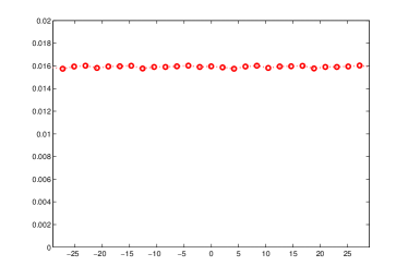
Figure 1: DOS of the hermitian Zakharov-Shabat eigenvalue problem as a function of the eigenvalue $\lambda$. The eigenvalues were found by direct diagonalization, using an adaptation of the modified Ablowitz-Ladik scheme ($D=1$, $\mbox{size}=20$, $\mbox{step}=0.1$, $200$ runs). We see the independence of the DOS from $\lambda$.

Beyond determining the DOS, we want to know whether the eigenvalues are statistically independent, i.e. whether $\rho(\lambda,\lambda^{\prime})=\rho(\lambda)\rho(\lambda^{\prime})$. We were able to show this both analytically and numerically. On the analytical side, we used Halperin’s method Halperin (1965); Frisch and Lloyd (1960). We define the variables $\theta(x)=\mbox{arg}\left(\frac{\psi_{1}(x)}{\psi_{2}(x)}\right)$, $\theta^{\prime}(x)=\mbox{arg}\left(\frac{\psi_{1}^{\prime}(x)}{\psi_{2}^{\prime}(x)}\right)$. Their evolution along $x$ is a Markov process and from (15) we can derive the Fokker-Planck equation for their probability distribution $P(x;\theta,\theta^{\prime})$:

$$\frac{\partial P}{\partial x} = \lambda\frac{\partial P}{\partial\theta}+\lambda^{\prime}\frac{\partial P}{\partial\theta^{\prime}}+D\left(\frac{\partial^{2}P}{\partial\theta^{2}}+\frac{\partial^{2}P}{\partial{\theta}^{2}}\right)$$

$$+ 2D\frac{\partial^{2}}{\partial\theta\partial\theta^{\prime}}\left(\cos(\theta-\theta^{\prime})P\right).$$

We also derive the equation for the quantity $F(x;\theta\theta^{\prime})\equiv\left\langle\frac{\partial\theta}{\partial\lambda}\frac{\partial\theta^{\prime}}{\partial\lambda^{\prime}}\delta(\theta(x)-\theta)\delta(\theta^{\prime}(x)-\theta^{\prime})\right\rangle$ (the brackets denote averaging over the gaussian ensemble of $u$’s)

$$\frac{\partial F}{\partial x} = -H-G+\lambda\frac{\partial F}{\partial\theta}+\lambda^{\prime}\frac{\partial F}{\partial\theta^{\prime}}$$

$$+ D\left(\frac{\partial^{2}F}{\partial\theta^{2}}+\frac{\partial^{2}F}{\partial{\theta}^{2}}\right)+2D\cos(\theta-\theta^{\prime})\frac{\partial^{2}F}{\partial\theta\partial\theta^{\prime}}$$

where $H(x;\theta,\theta^{\prime})$, $G(x;\theta,\theta^{\prime})$ satisfy the same equation as $P(x;\theta,\theta^{\prime})$ but with $-P$ as an extra source term. $F$ grows as $\rho(\lambda,\lambda^{\prime})\times x^{2}$ for large $x$ and from (II),(II) we are able to calculate $\rho(\lambda,\lambda^{\prime})$ and show that it factorizes.

Numerically, we find the distribution of the distances between neighboring eigenvalues. Statistical independence means that the distances must follow a Poisson distribution, and this is indeed what we find. The results are shown in FIG. 2

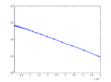
Figure 2: Logarithmic plot of the distribution of the distance between successive eigenvalues of the hermitian Zakharov-Shabat operator ($D=1$, $\mbox{size}=100$, $\mbox{step}=0.1$, $100$ runs). The linearity of the data shows that the distances follow a Poisson distribution, i.e. there is no bias in the magnitude of the distance, in agreement with our theoretical result about statistical independence of eigenvalues even in the dense soliton limit.

The effect of (weak) additive noise coming from periodic amplification on the eigenvalues can be studied in the context of adiabatic perturbation theory and the IST Lashkin (2004). It is thus shown that for white gaussian noise, the disturbance of the eigenvalues is gaussian, with zero mean and a variance $\left\langle\Delta\lambda^{2}\right\rangle$ proportional to the strength of the noise and the inverse participation ratio $\int dx||\psi||^{4}$ of the corresponding (normalized) eigenstates. The inverse participation ratio (IPR)in the many soliton situation that we are interested in is beyond analytical treatment. In the next two figures we show the results of numerical simulations where we calculated the IPR for the eigenstates of $U_{H}$ found using direct diagonalization of $U_{H}$ with a central differences discretization (in order to impose zero boundary conditions at the edges).

In FIG. 3 we see how the IPR (locally averaged for smoothness) behaves as a function of the eigenvalue $\lambda$ for a given $D$. We are actually interested only in the middle, flat section, because the raising of the edges is an artefact of the central difference method that creates an over-concentration of eigenvalues near the edges of the spectrum.

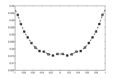
Figure 3: Inverse participation ratio as a function of the eigenvalue $\lambda$, for a given average power of the input ($D=1$, $\mbox{size}=100$, $\mbox{step}=0.1$, $100$ runs).

Averaging over this flat segment for different $D$’s, we see in FIG. 4 the dependence of $\int dx||\psi||^{4}$ on the average input power $D$. The linearity indicates that the IPR is actually proportional to the localization length (the inverse Lyapunov exponent) of $U_{H}$ Bartosch (2000).

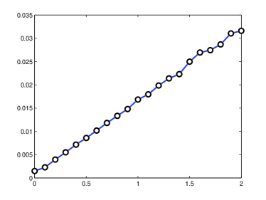
Figure 4: Inverse participation ratio, averaged over the eigenvalues, as a function of the average input power $D$ ($\mbox{size}=100$, $\mbox{step}=0.1$, $100$ runs).

III Bright Solitons

The non-hermitian Zakharov-Shabat eigenvalue problem is defined by the system of equations

$$\begin{array}[]{l}{\mbox{\boldmath{$U$}}}{\mbox{\boldmath{$\psi$}}}(x)=z{\mbox{\boldmath{$\psi$}}}(x),\\ \\ {\mbox{\boldmath{$U$}}}=\left(\begin{array}[]{lr}i\frac{\partial}{\partial x}&u^{*}(x,0)\\ -u(x,0)&-i\frac{\partial}{\partial x}\end{array}\right),\\ \\ {\mbox{\boldmath{$\psi$}}}(x)=\left(\begin{array}[]{c}\psi_{1}(x)\\ \psi_{2}(x)\end{array}\right).\end{array}$$ (28)

on the infinite line, together with the boundary conditions $\psi_{1},\psi_{2}\to 0$ as $x\to\pm\infty$. The star denotes complex conjugation, and the eigenvalue $z=\xi+i\eta$ is generally complex. As in the hermitian case, the “potential” $u(x,0)$ is the envelope of the electric field that goes into the fiber. We want to find the density of states (DOS) of this operator when $u$ is gaussian random, as in (16). The DOS $\rho(\xi,\eta)$ of this random operator determines the entropy of information carried by the gaussian signal through the formula $I=-\int d\xi d\eta\rho(\xi,\eta)\log\rho(\xi,\eta)$.

Contrary to its hermitian counterpart, this DOS is not known in the literature. Halperin’s method Halperin (1965), which works so nice for the hermitian/dark soliton case, fails here because of non-hermiticity. Non-hermitian random operators have received considerable attention in the literature (see Marchetti and Simons (2001) for a list of important references on the subject). They have a wide range of applications, in non-equilibrium statistical mechanics, random classical dynamics, the physics of polymers, QCD, neural networks, and, in the case at hand, soliton physics and communications. Non-hermiticity means that the eigenvalues migrate to the complex plane. This complicates the computation of their statistical properties - most notably their DOS - relative to hermitian operators. The underlying reason for this is that the propagator in the hermitian case is analytic except on branch cuts of the real axis, where the real eigenvalues condense. This introduces constraints that facilitate the computation of the DOS. When the eigenvalues are complex this is no longer true. In many cases however one can obtain approximate results for the DOS. The hermitization method, developed by Feinberg and Zee in Feinberg and Zee (1997) can be applied here. The method gives the self-consistent Born approximation (SCBA) to the density of states. Instead of looking at $U$ directly, one starts with a “hermitized” operator

$${\mbox{\boldmath{$H$}}}=\left(\begin{array}[]{lr}0&{\mbox{\boldmath{$U$}}}-z\\ &\\ {\mbox{\boldmath{$U$}}}^{\dagger}-z^{*}&0\end{array}\right)$$ (32)

and calculates the propagator ${\mbox{\boldmath{$G$}}}=\frac{1}{\mu-{\mbox{\boldmath{$H$}}}}$ in the SCBA. The DOS is then given by the derivative with respect to $z^{*}$ of the trace of the lower-left block of $G$. We omit the details of the calculation and state only the final result. We find the DOS to be uniform inside a uniform band centered around the $\xi$ axis on the complex $z$ plane, with the width being proportional to $D$:

$$\rho(\xi,\eta)=\left\{\begin{array}[]{cl}\frac{1}{2\pi D},&|\eta|\leq D\\ &\\ 0,&|\eta|>D\end{array}\right.$$ (36)

To move beyond the SCBA, and see how the DOS “frays” near the edges of the band, we used the method of optimal fluctuations Zittartz and Langer (1966); Izyumov and Simons (1999). The basic idea is that states outside the band given by the SCBA are created by atypically strong fluctuations of the “potential” $u(x,0)$. Such fluctuations occur with an exponentially small probability $\exp\left[-W/D\right]$, where

$$W=\frac{1}{2}\int dx|u(x,0)|^{2}.$$ (37)

Minimizing the functional $W[u]$ in (37) with respect to $u$, with the additional constraint $\det({\mbox{\boldmath{$U$}}}-z)=0$ enforced as a Lagrange multiplier, we can determine the density of states outside the band with exponential accuracy. The minimization involves the solution of a pair of coupled nonlinear ordinary differential equations and the result for the optimal potential is:

$$u(x)=4i\eta\left(\frac{e^{2\eta x}+e^{-2\eta x}}{e^{4\eta x}+e^{-4\eta x}+2}\right)e^{-2i\xi x}.$$ (38)

From (37,38) we then find that to exponential accuracy, the DOS for $|\eta|\gg D$ is

$$\rho(\xi,\eta)\sim e^{-\frac{4|\eta|}{D}}.$$ (39)

Although these approximate methods provide some measure of knowledge of the DOS (and consequently the entropy of information of the gaussian random signal), an exact expression is always desirable, for obvious reasons. We were able to obtain such a result using a variation of the Thouless formula Thouless (1972), that relates the DOS with the Lyapunov exponent of the operator $U$ in (28). The Lyapunov exponent $\lambda$ measures the rate of exponential increase of the modulus of a typical solution of (28) as one goes towards larger $x$ with no boundary conditions are imposed. One possible definition is:

$$\lambda=\lim_{x\to\infty}\frac{1}{x}\ln\left(|\psi_{1}(x)|^{2}+|\psi_{2}(x)|^{2}\right)^{\frac{1}{2}}.$$ (40)

We were able to show that for any set of finite boundary conditions, a unique, positive Lyapunov exponent exists and it is related to the DOS by the formula

$$\rho(\xi,\eta)=\frac{1}{2\pi}\left(\frac{\partial^{2}}{\partial\xi^{2}}+\frac{\partial^{2}}{\partial\eta^{2}}\right)\lambda(\xi,\eta).$$ (41)

The eigenvalue problem (28) has enough symmetry to make the exact calculation of $\lambda$ (and from this, $\rho$) possible. The details of this calculation are contained in the attached paper (together with the detailed proof of (41) and the relevant references) which has been published in Phys. Rev. E Kazakopoulos and Moustakas (2008). The expression we arrive at for the DOS is:

$$\rho(\xi,\eta)=\frac{2}{\pi D}\frac{\frac{2\eta}{D}\coth\left(\frac{2\eta}{D}\right)-1}{\sinh^{2}\left(\frac{2\eta}{D}\right)}$$ (42)

We have also been able to show that (42)remains valid for large $\xi$ in the case of a purely real gaussian random potential that maximally breaks rotational symmetry (completely polarized input). The comparison of this prediction with numerical simulations is shown in FIG. 5.

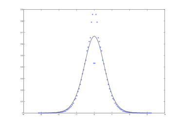
Figure 5: Theoretical curve (solid line) and results of numerical simulations for the profile of the DOS vs. $\eta$. We have used the modified Ablowitz-Ladik diagonalization scheme Weideman and Herbst (1997). The value of $D$ is $1$, the size of the system is $L=135$ and the step size is $0.075$. The disturbance near $\eta=0$ is a finite-size effect. The localization length $l=\lambda^{-1}$ grows as $l\sim 3D/2\eta^{2}$ near $\eta=0$ and so numerical results become unreliable for $|\eta|\lesssim\sqrt{D/L}$ ($\sim 0.1$ here).

This description of the input signal in terms of the density of $\xi$ and $\eta$ is complete only in the cases where one can neglect the effects of jitter in the positions of the solitons and concentrate on the shift in the eigenvalues as the primary cause of signal distortion. If we want to include the positional jitter, we must take into account the information contained in the positions of the solitons. This is done by considering another set of complex numbers $b_{z}$, one for each solitonic excitation, which are associated with soliton positions and together with the eigenvalues fully determine the solitonic part of the signal. Since we study the effects of noise on a random Gaussian input pulse, where all eigenstates are localized in the infinite pulse duration limit, the eigenvalues $z$ and and the corresponding $b_{z}$ give a complete description of the signal.

We were able to compute the distribution of $b_{z}$ resulting from a random gaussian input analytically by using the definition of $b_{z}$ and expressing it in terms of the behavior of the eigenfunctions at the edges of the pulse, which in turn we can express as sums of random variables with calculable distributions. More specifically, the precise asymptotic conditions for the eigenfunctions are:

$$\begin{array}[]{l}{\mbox{\boldmath{$\Psi$}}}_{z}(x)\rightarrow\left(\begin{array}[]{c}0\\ 1\end{array}\right)e^{izx},\;\;\bar{{\mbox{\boldmath{$\Psi$}}}}_{z}(x)\rightarrow\left(\begin{array}[]{c}1\\ 0\end{array}\right)e^{-izx}\;\;\;\;\mbox{as}\;\;x\rightarrow\infty\\ \\ {\mbox{\boldmath{$\Phi$}}}_{z}(x)\rightarrow\left(\begin{array}[]{c}1\\ 0\end{array}\right)e^{-izx},\;\bar{{\mbox{\boldmath{$\Phi$}}}}_{z}(x)\rightarrow\left(\begin{array}[]{c}0\\ 1\end{array}\right)e^{izx}\;\;\;\;\mbox{as}\;\;x\rightarrow-\infty.\end{array}$$ (54)

where the two sets of solutions are related through an S-matrix:

$$\left[\begin{array}[]{c}{\mbox{\boldmath{$\Phi$}}}_{z}(x)\\ \bar{{\mbox{\boldmath{$\Phi$}}}}_{z}(x)\end{array}\right]=\left(\begin{array}[]{cc}b(z)&a(z)\\ \bar{a}(z)&\bar{b}(z)\end{array}\right)\left[\begin{array}[]{c}{\mbox{\boldmath{$\Psi$}}}_{z}(x)\\ \bar{{\mbox{\boldmath{$\Psi$}}}}_{z}(x)\end{array}\right]$$ (61)

with the $a$, $b$’s being the transmission and reflection coefficients respectively. By taking into account the symmetry of the problem under complex conjugation it is possible to show that $a(z^{*})=\bar{a}^{*}(z)$ and $b(z^{*})=-\bar{b}^{*}(z)$, where the star (^∗) denotes the complex conjugate.

When the above solutions correspond to a localized eigenfunction with eigenvalue $z$, the transmission coefficient $a(z)$ has to vanish at that $z$, making the two sets of solutions directly proportional:

$$\begin{array}[]{c}{\mbox{\boldmath{$\Phi$}}}_{z}(x)=b_{z}{\mbox{\boldmath{$\Psi$}}}_{z}(x)\\ \\ \bar{{\mbox{\boldmath{$\Phi$}}}}_{z}(x)=-b_{z}^{*}\bar{{\mbox{\boldmath{$\Psi$}}}}_{z}(x)\end{array}$$ (65)

where $\Phi_{z}$ and $\bar{\Phi}_{z}$ are the admissible exponentially decaying eigenfunctions for $Im(z)>0$ and $Im(z)<0$, respectively. Then, for $\eta>0$ we have from (54,65)

$$\begin{array}[]{c}{\mbox{\boldmath{$\Psi$}}}_{z}(x)\rightarrow\left(\begin{array}[]{c}0\\ 1\end{array}\right)e^{izx}\;\mbox{as}\;x\rightarrow\infty\\ \\ {\mbox{\boldmath{$\Psi$}}}_{z}(-x)\rightarrow\left(\begin{array}[]{c}b_{z}^{-1}\\ 0\end{array}\right)e^{izx}\;\mbox{as}\;x\rightarrow\infty\end{array}$$ (73)

Defining $\tilde{{\mbox{\boldmath{$\Psi$}}}}_{z}(x)\equiv{\mbox{\boldmath{$\Psi$}}}_{z}(-x)$ we can write:

$$b=\lim_{x\to\infty}b(x),\;\;\;b(x)\equiv\frac{\psi_{2}(x)}{\tilde{\psi}_{1}(x)},$$ (74)

where for convenience we have dropped the subscript $z$. The time evolution of $\ln{b}$ is found from (28),

$$\frac{\partial\ln{b}}{\partial x}=i\left(uf+\tilde{u}^{*}\tilde{f}\right)$$ (75)

with $f(x)=\frac{\psi_{1}}{\psi_{2}}$, $\tilde{f}(x)=\frac{\tilde{\psi}_{2}}{\tilde{\psi}_{1}}$, $\tilde{u}(x)\equiv u(-x)$, and

$$\begin{array}[]{l}\frac{\partial f}{\partial x}=-2izf+iu^{*}-iuf^{2}\\ \\ \frac{\partial\tilde{f}}{\partial x}=-2iz\tilde{f}-i\tilde{u}+i\tilde{u}^{*}\tilde{f}^{2}.\end{array}$$ (79)

Eqs. (75,79) can be used to write down a Fokker-Planck equation for the probability distribution of $\ln b_{z}$. The stationary solution of this equation is the actual distribution of $\ln b_{z}$ in the infinite pulse limit, and it turns out to be uniform, as we would expect from the translational invariance of the input signal. The precise way in which this happens can be found by using (75) to express $\ln b_{z}$ as a sum of random variables with known limit distribution. The details of this calculation together with the relevant references are included in the attached paper. The result is a Gaussian distribution for the real part of $\ln b_{z}$ in the case of an unpolarized incoming pulse, with zero mean and variance growing as:

$$\sigma^{2}=4\sqrt{\pi}\frac{\eta e^{\frac{2\eta}{D}}}{\sinh\left(\frac{2\eta}{D}\right)}T\ln\frac{T}{2\tau},$$ (80)

where $T$ is the duration of the incoming pulse and $\tau$ is the inverse bandwidth. The imaginary part of $\ln b$ is an angle and so, although it follows the same distribution as the real part, will due to periodicity become uniformly distributed in $[0,2\pi)$.

For a completely polarized incoming pulse, the distribution of $\ln|b_{z}|$ will asymptotically follow a Cauchy distribution scaling like $T/\tau$. Its statistical median will be zero by symmetry. The phase of $b$ will again be uniform over $[0,2\pi)$, although the mechanism is different in this case. For the special case of $\xi=0$, the scale parameter of the Cauchy distribution can be calculated more explicitly to be

$$\gamma\sim\frac{e^{\eta/D}}{I_{0}(\eta/D)}\frac{T}{\tau}$$ (81)

where $I_{0}$ is a modified Bessel function of the first kind.

IV Optical Fiber Channel Capacity

Armed with the knowledge of the distributions of scattering data $\{z,b_{z}\}$ generated by a random Gaussian input signal, we address the question of the capacity, or spectral efficiency, of the optical fiber channel. Historically, there has been a steady exponential increase in the transmission capacity of fiber optics communications systems, resulting mainly from higher transmission rates and the implementation of wavelength division multiplexing (WDM). WDM systems generally use binary on-off keying as their signaling scheme, thus limiting the spectral efficiency (bits transmitted per second per Hz of bandwidth) to 1 b/s/Hz. More complicated signaling schemes can go beyond this limit, and will eventually be required in order to make use of the potential of the optical fiber network. Some amount of interesting work has been done on the question of the capacity limits for WDM and related systems, both analytical and numerical (see Mitra and Stark (2001); Stark et al. (2001); Narimanov and Mitra (2002); Green et al. (2002); Turitsyn et al. (2003); Kahn and Ho (2004); Djordjevic et al. (2005); Ivcovic et al. (2007); Mecozzi and Shtaif (2001); Mecozzi (1994); Peddanarappagari and Brandt-Pearce (1997); Ho (2005) and references therein). In particular, in Mitra and Stark (2001) the spectral efficiency predicted is about $8.5bits/sec/Hz$, in the absence of jitter. In our model we consider a single-channel mode instead of the multi-channel setup of WDM. This has the advantage of avoiding the multiplicative noise resulting from interference between different channels. The modulation of the very large bandwidth of optical fibers ($\sim$ 50 THz) is beyond the ability of current electronic equipment, but we are interested in the limits posed by the very physics of nonlinearity, which future technological advances should be able to approach.

The use of a definite input signal (random Gaussian) provides a lower bound for the capacity of the system, since the Gaussian is not necessarily the optimal input distribution for nonlinear channels. As we said in the introduction, the method we use is a transformation to the field of eigenvalues of the Zakharov-Shabat operator, where the amplifier noise becomes additive. We consider a system consisting of a fiber span of total length $L$, and $N_{a}$ equally spaced identical amplifiers that compensate for the loss of strength in the signal while unavoidably injecting it with white noise (amplified spontaneous emission noise or ASE noise). For long-range transmission systems $L\sim 1000\mbox{km}$ and the inter-amplifier spacing is $L_{a}\sim 50-100\mbox{km}$. We study the case of bright solitons only, since dark solitons are not used for large distance communications. Mathematically it is modeled by the addition of a term $i\sum_{n=1}^{N_{a}}\delta\left(x-nL_{a}\right)f_{n}(t)$ on the rhs of Eq. (2) with the roles of space and time interchanged. The delta-correlated white noise added at each amplifier has noise strength Moore et al. (2006)

$$\left<f_{n}(t)f_{m}(t^{\prime})\right>=\sigma^{2}\delta_{nm}\delta(t-t^{\prime}),\;\;\;\sigma^{2}=\frac{h\nu_{0}\eta_{sp}(G-1)^{2}}{G\ln G},$$ (82)

where $h$ is Planck’s constant, $\nu_{0}$ is the carrier frequency, $\eta_{sp}$ is the spontaneous emission factor and $G=e^{\alpha L_{a}}$ is the amplification factor ($\alpha=0.2\mbox{dB/km}$). The noise causes a random shift in the eigenvalues:

$$z_{\mbox{out}}=z_{\mbox{in}}+\delta z.$$ (83)

As long as the signal to noise ratio, which can be increased by increasing the input power or reducing the distance between amplifiers, is large, $\delta z$ (or rather its variance) can be calculated using adiabatic perturbation theory:

$$\delta z=\frac{1}{2i}\frac{\int\left(f\psi_{1}^{2}+f^{*}\psi_{2}^{2}\right)}{\int\psi_{1}\psi_{2}}.$$ (84)

The denominator here is the non-Hermitian norm of the eigenvector. The second moments of $\delta z$, $\left<\delta z^{2}\right>$ and $\left<|\delta z|^{2}\right>$ contain integrals of the form $\int\psi_{1}^{2}\psi_{2}^{2}$ that do not correspond to integrals of the motion and it is hard, if at all possible, to calculate them analytically. They can however be evaluated numerically, using the eigenstates corresponding to each eigenvalue .

The rate (per Hz) of information transmission in our model (ignoring jitter for the moment) is given by:

$$R=H[z_{out}]-\left\langle H[z_{out}|z_{in}]\right\rangle_{p_{z_{in}}}.$$ (85)

Since we work in the perturbative regime, we can consistently approximate $H[z_{out}]$ with $H[z_{in}]$, and because the noise is additive, $H[z_{out}|z_{in}]=H[\delta z]$. Thus we arrive at a simplified formula for the rate:

$$R=H[z_{in}]-H[\delta z].$$ (86)

The entropy of $z_{in}$ is calculated from the distribution of eigenvalues given in the previous section: $P(\xi,\eta)=P_{\xi}(\xi)P_{\eta}(\eta)$. Only positive values of $\xi$ and $\eta$ correspond to independent eigenstates, the rest being “mirror images” of these . $\xi$ is uniformly distributed, with maximum value $\Lambda=2\pi B$, where $B$ is the bandwidth, and $\eta$ is distributed according to:

$$P_{\eta}(\eta)=\frac{4}{D}\frac{\frac{2\eta}{D}\coth\left(\frac{2\eta}{D}\right)-1}{\sinh^{2}\left(\frac{2\eta}{D}\right)}.$$ (87)

The incoming entropy (per symbol,in nats) then is:

$$H[\xi,\eta]=H[\xi]+H[\eta]=\ln\Lambda+\ln\left(\frac{D}{4}\right)+0.08\;.$$ (88)

The entropy of the noise is computed in the Gaussian approximation , as the logarithm of the covariance matrix of $\delta\xi,\delta\eta$. The distribution of the logarithm of eigenvalues of this matrix for a value of $D=2$ is shown in FIG. 6.

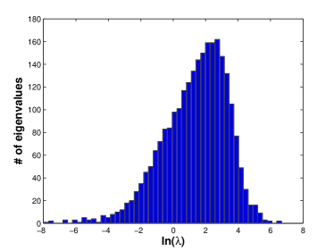
Figure 6: Distribution of the logarithm of the eigenvalues of the covariant matrix. The value of $D$ is $2$, the size of the system is $L=150$ and the step size is $0.06$.

The entropy (per symbol) of the noise in the Gaussian approximation is:

$$H[\delta z]=\ln\left((2\pi e)^{\frac{1}{2}}\bar{\lambda}\right)$$ (89)

where $\bar{\lambda}$ is the geometric mean of the eigenvalues of the ($2N\times 2N$, $N$ being the number of eigenvalues) covariance matrix of $\delta\xi_{i},\delta\eta_{i}$, $C_{ij}$. In FIG. 7 we see a plot of $\bar{\lambda}\over{\sigma^{2}}$ for ten values of $D$.

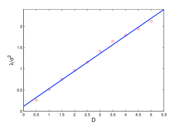
Figure 7: The geometric mean of the eigenvalues of the covariance matrix as a function of the signal strength $D$. The solid line is a linear fit. The size of the system is $L=150$ and the step size is $0.06$.

The linear fit gives $\bar{\lambda}=0.41\sigma^{2}D$, and allows us to compute a first result for the spectral efficiency lower bound (again, ignoring jitter):

$$R=\ln\left(\left(\frac{\pi}{8e}\right)^{\frac{1}{2}}\frac{BG\ln G}{0.41h\nu_{0}\eta_{sp}(G-1)^{2}}P_{c}t_{c}^{2}\right)$$ (90)

where $P_{c},t_{c}$ are the characteristic units of power and time used to normalize the units of the NLSE and they are inserted here to express the result in SI units. For a system with $N_{a}$ amplifiers, one needs to replace $\sigma^{2}$ with $N_{a}\sigma^{2}$. Plugging in typical values for the quantities involved ($P_{c}=0.05W,t_{c}=3\times 10^{-11}s,G=100,\eta_{sp}=2,h=6.6\times 10^{-34}J\cdot s,\nu_{0}=2\times 10^{14}Hz,N_{a}=10$) we find:

$$R=\ln\left(7\times 10^{-7}\times B\right)\;\mbox{bits/s/Hz}$$ (91)

with the bandwidth $B$ measured in Hz. Using all the available bandwidth for optical fibers, $B=50\mbox{THz}$ this yields a value of $R\simeq 25\mbox{bits/s/Hz}$, which is significantly higher than the predicted result for the case of WDM Mitra and Stark (2001). One thing to note about this result is that $D$ altogether disappears, cancelling between the incoming entropy and the noise. This is because the variance of the eigenvalue shift is linear in $D$. This is in contrast to analogous results in WDM models, where increasing the signal strength also increases the multiplicative noise between channels and the capacity falls after reaching a maximum for a finite value of the SNR Mitra and Stark (2001); Stark et al. (2001); Narimanov and Mitra (2002); Green et al. (2002); Kahn and Ho (2004).

However, this result is incomplete as long as it does not include the effects of jitter, which could significantly reduce the capacity. To do this we need to consider not just the eigenvalues $\{z\}$, but also the $\{\ln b_{z}\}$, so that the signal description is complete . The evolution of $\ln b_{z}$ is given by Konotop and Vásquez (1994):

$$\begin{array}[]{l}\frac{\partial\ln|b_{z}|}{\partial x}=8\xi\eta\\ \\ \frac{\partial\phi}{\partial x}=4(\eta^{2}-\xi^{2})\end{array}$$ (95)

so that $\ln b_{z}$ is affected by the noise in $\xi$ and $\eta$. There is also noise specific to $\ln b_{z}$ at each amplifier, but this is bounded and can be neglected for long-range transmission. To properly include the $\{\ln b_{z}\}$ in our scheme and get a reliable lower bound for the capacity we must ascertain their correlations, which we have found to be non-zero. We are currently attempting to find an analytic expression for the correlations. If this proves impossible, we shall compute their correlation matrix numerically starting from (75) and use it to compute the incoming entropy. Since the $\{\ln b_{z}\}$ follow a Gaussian distribution, this does not spoil the lower bound feature.

References

- Hasegawa and Tappert (1973a) A. Hasegawa and F. Tappert, Applied Physics Letters 23, 142 (1973a).
- Hasegawa and Tappert (1973b) A. Hasegawa and F. Tappert, Applied Physics Letters 23, 171 (1973b).
- Drazin and Johnson (1989) P. G. Drazin and R. S. Johnson, Solitons: An Introduction (Cambridge University Press, 1989).
- Konotop and Vásquez (1994) V. V. Konotop and L. Vásquez, Nonlinear Random Waves (World Scientific, Singapore, 1994).
- Shannon (1948) C. E. Shannon, Bell System Technical Journal 27, 379 (1948).
- Cover and Thomas (1991) T. M. Cover and J. A. Thomas, Information Theory (John Wiley and Sons, Inc., New York, NY, 1991).
- Glass et al. (2000) A. M. Glass, D. J. DiGiovanni, T. A. Strasser, R. E. S. Andrew J. Stentz, A. E. White, A. R. Kortan, and B. J. Eggleton, Bell Labs Technical Journal 5, 168 (2000).
- Mitra and Stark (2001) P. P. Mitra and J. B. Stark, Nature 411, 1027 (2001).
- Stark et al. (2001) J. B. Stark, P. Mitra, and A. Sengupta, Optical Fiber Technology 7, 275 (2001).
- Narimanov and Mitra (2002) E. Narimanov and P. P. Mitra, Journal of Lightwave Technology 20, 530 (2002).
- Green et al. (2002) A. G. Green, P. B. Littlewood, P. P. Mitra, and L. G. L. Wegener, Phys. Rev. E 66, 046627 (2002).
- Turitsyn et al. (2003) K. S. Turitsyn, K. A. Derevyanko, I. V. Yurkevich, and S. K. Turitsyn, Physical Review Letters 91, 203901 (2003).
- Kahn and Ho (2004) J. M. Kahn and K.-P. Ho, IEEE Journal of Selected Topics in Quantum Electronics 10, 259 (2004).
- Agrawal (1992) G. P. Agrawal, Fiber-Optic Communication Systems (J. Wiley & Sons, New York, 1992).
- Kaminow and Koch (1997) I. P. Kaminow and T. L. Koch, eds., Optical Fiber Telecommunications IIIA (Academic Press, San Diego, CA, 1997).
- Gordon and Haus (1986) J. P. Gordon and H. A. Haus, Optics Letters 11, 665 (1986).
- Kivshar et al. (1994) Y. S. Kivshar, M. Haelterman, P. Emplit, and J. P. Hamaide, Optics Letters 19, 19 (1994).
- Mollenauer et al. (1992) L. F. Mollenauer, J. P. Gordon, and S. G. Evangelides, Optics Letters 17, 1575 (1992).
- Nakazawa et al. (1991) M. Nakazawa, E. Yamada, H. Kubota, and K. Suzuki, Electronics Letters 27, 1270 (1991).
- Forysiak and Doran (1995) W. Forysiak and N. J. Doran, Journal of Lightwave Technologies 13, 850 (1995).
- Goedde et al. (1995) C. G. Goedde, W. L. Kath, and P. Kumar, Optics Letters 20, 1365 (1995).
- Essiambre and Agrawal (1997) R. J. Essiambre and G. P. Agrawal, Journal of the Optical Society of America B 14, 323 (1997).
- Karter et al. (1997) G. M. Karter, J. M. Jacob, C. R. Meynuk, E. A. Golovchenko, and A. N. Pilipetskii, Optics Letters 22, 513 (1997).
- McKinstrie et al. (2002) C. J. McKinstrie, J. Santhanam, and G. P. Agrawal, Journal of the Optical Society of America B 19, 640 (2002).
- Zakharov and Shabat (1972) V. E. Zakharov and A. B. Shabat, Sov. Phys. JETP 34, 62 (1972).
- Ovchinnikov and Erikhman (1977) A. A. Ovchinnikov and N. S. Erikhman, Sov. Phys. JETP 46, 340 (1977).
- Hayn and John (1987) R. Hayn and W. John, Zeitschrift für Physik B 67, 169 (1987).
- Gredeskul et al. (1990) S. A. Gredeskul, Y. S. Kivshar, and M. V. Yanovskaya, Phys. Rev. A 41, 3994 (1990).
- Bartosch (2000) L. Bartosch, Ph.D. thesis, University of Göttingen, Göttingen (2000), URL http://webdoc.sub.gwdg.de/diss/2000/bartosch/thesis.pdf.
- Weideman and Herbst (1997) J. A. C. Weideman and B. M. Herbst, Mathematics and Computers in Simulation 43, 77 (1997).
- Halperin (1965) B. I. Halperin, Phys. Rev. 139, A104 (1965).
- Frisch and Lloyd (1960) H. L. Frisch and S. P. Lloyd, Physical Review 120, 1175 (1960).
- Lashkin (2004) V. M. Lashkin, Physical Review E 70, 066620 (2004).
- Marchetti and Simons (2001) F. M. Marchetti and B. D. Simons, Journal of Physics A: Mathematical and General 34, 10805 (2001).
- Feinberg and Zee (1997) J. Feinberg and A. Zee, Nuclear Physics B 504, 579 (1997).
- Zittartz and Langer (1966) J. Zittartz and J. S. Langer, Physical Review 148, 741 (1966).
- Izyumov and Simons (1999) A. V. Izyumov and B. D. Simons, Physical Review Letters 83, 4373 (1999).
- Thouless (1972) D. J. Thouless, Journal of Physics C: Solid State Physics 5, 77 (1972).
- Kazakopoulos and Moustakas (2008) P. Kazakopoulos and A. L. Moustakas, Phys. Rev. E 78, 016603 (2008).
- Djordjevic et al. (2005) I. B. Djordjevic, B. Vasic, M. Ivcovic, and I. Gabitov, Journal of Lightwave Technology 23, 3755 (2005).
- Ivcovic et al. (2007) M. Ivcovic, I. B. Djordjevic, and B. V. M. Ivcovic, Journal of Lightwave Technology 25, 1163 (2007).
- Mecozzi and Shtaif (2001) A. Mecozzi and M. Shtaif, IEEE Photonics Technology Letters 13, 1029 (2001).
- Mecozzi (1994) A. Mecozzi, Journal of Lightwave Technology 12, 1993 (1994).
- Peddanarappagari and Brandt-Pearce (1997) K. V. Peddanarappagari and M. Brandt-Pearce, Journal of Lightwave Technology 15, 2232 (1997).
- Ho (2005) K.-P. Ho, IEEE Photonics Technology Letters 17, 858 (2005).
- Moore et al. (2006) R. O. Moore, G. Biondini, and W. L. Kath, CAMS Report 0506-35 (2006).