Electrical conductivity of quark matter at finite $T$

Abstract

In this talk, I present the recent theoretical results on the electrical conductivity (EC) $\sigma$ of quark matter, using the Kubo formula at finite temperature and zero quark density $(T\neq 0,\mu=0)$ in the presence of an external strong magnetic field. The dilute instanton-liquid model with the caloron distribution is taken into account. It turns out that $\sigma\approx(0.02\sim 0.15)\,\mathrm{fm}^{-1}$ for $T=(0\sim 400)$ MeV with the relaxation time $\tau=(0.3\sim 0.9)$ fm. EC is parameterized as $\sigma/T\approx(0.46,0.77,1.08,1.39)\,C_{\mathrm{EM}}$ for $\tau=(0.3,0.5,0.7,0.9)$ fm, respectively. These results are well compatible with other theoretical estimations and show almost negligible effects from the magnetic field. The soft photon emission rate from the quark-gluon plasma is discussed as well.

I Introduction

The observation of the strong magnetic field in the peripheral heavy-ion collision at Relativistic Heavy Ion Collider (RHIC) of BNL Voloshin:2008jx triggered abundant related research works Kharzeev:2004ey ; Buividovich:2009wi ; Fukushima:2008xe ; Kharzeev:2010gd ; Nam:2011vn ; Ding:2010ga ; Kerbikov:2012vp . The transport coefficients for the hot and/or dense matter play an important role in general as well, since they determine the physical properties of the matter, being studied by the Kubo formula BOOKEM . In the present work, I would like to investigate the electrical conductivity (EC) $\sigma$, relating to the vector-current correlation (VCC) in the presence of the external static magnetic field $\bm{B}$. EC was investigated in the hot phase of the QCD plasma and extracted from a quenched SU($N_{c}$) lattice QCD (LQCD) in Refs. Ding:2010ga ; Gupta:2003zh . Beside LQCD, The authors explored EC using the Green-function method Kerbikov:2012vp . Note that EC is deeply related to the thermal dilepton production from the quark-gluon plasma (QGP) Harada:2006hu . To this end, I will use the dilute instanton-liquid model Shuryak:1981ff ; Diakonov:1983hh , modified by the caloron Diakonov:1988my ; Nam:2009nn , resulting in that the instanton size $\bar{\rho}$ becomes a smoothly decreasing function of $T$, signaling weakening nonperturbative effects of QCD. From the numerical results, it turns out that $\sigma\approx(0.02\sim 0.15)\,\mathrm{fm}^{-1}$ for $T=(0\sim 400)$ MeV with the relaxation time $\tau=(0.3\sim 0.9)$ fm. In addition, The parameterization of EC is given as $\sigma/T\approx(0.46,0.77,1.08,1.39)\,C_{\mathrm{EM}}$ for $\tau=(0.3,0.5,0.7,0.9)$ fm, respectively. These results are well compatible with other theoretical estimations and show almost negligible effects from the magnetic field. The soft photon emission rate from the quark-gluon plasma is discussed as well.

II Theoretical framework

First, EC can be defined in Euclidean space from the Kubo formula Kerbikov:2012vp :

$$\sigma_{\mu\nu}(p)=-\sum_{f}\frac{e^{2}_{f}}{w_{p}}\int\frac{d^{4}k}{(2\pi)^{4}}\mathrm{Tr}_{c,\gamma}\left[S(k)\gamma_{\mu}S(k+p)\gamma_{\nu}\right]_{A}.$$ (1)

Here, $e_{f}$ stands for the electrical charge for a light-flavor ($f$) quark. $w_{p}$ indicates the Matsubara frequency for the momentum $p$ for $\sigma$, being proportional to $2\pi T$. $\mathrm{Tr}_{c,\gamma}$ is assigned as the trace over the color and Lorentz indices. In order to evaluate Eq. (1), the dilute instanton-liquid mode is employed Shuryak:1981ff ; Diakonov:1983hh . In Euclidean space, I define the effective chiral action (EChA) of the model:

$$\mathcal{S}_{\mathrm{eff}}=-\mathrm{Sp}_{c,f,\gamma}\ln\left[i\hbox to0.0pt{\,\,/\hss}{D}-iM(D^{2})\right],$$ (2)

where $\mathrm{Sp}_{c,f,\gamma}$ stands for the functional trace, while $M(D^{2})$ for the momentum-dependent effective quark mass with the U(1) covariant derivative $D_{\mu}$.The external electromagnetic (EM) field is induced to EChA via the Schwinger method Schwinger:1951nm . From EChA, one can derive the light-quark propagator under the external EM field in the momentum space as Nam:2009jb

$$S(K)\approx\frac{\hbox to0.0pt{\,/\hss}{K}+i[M_{k}+\frac{1}{2}\tilde{M}_{k}(\sigma\cdot F)]}{k^{2}+M^{2}_{k}},\,\,\,\,M_{k}=M_{0}\left[\frac{2}{2+\bar{\rho}^{2}k^{2}}\right]^{2},\,\,\,\,\tilde{M}_{k}=-\frac{8M_{0}\bar{\rho}^{2}}{(2+\bar{\rho}^{2}k^{2})^{3}},$$ (3)

where $K_{\mu}\equiv k_{\mu}+e_{f}A_{\mu}$ and $\sigma\cdot F\equiv\sigma_{\mu\nu}F^{\mu\nu}$. $M_{0}$ is determined as about $350$ MeV for $1/\bar{\rho}\approx 600$ MeV. Taking into account the $T$ dependence of $M$ as in Ref. Nam:2009nn , I can write the ($|k|,T$)-dependent $M$ as follows:

$$M_{k}=M_{0}\left[\frac{\sqrt{n(T)}\,\bar{\rho}^{2}(T)}{\sqrt{n(0)}\,\bar{\rho}^{2}(0)}\right]\left[\frac{2}{2+k^{2}\,\bar{\rho}^{2}(T)}\right]^{2}.$$ (4)

Considering all the ingredients discussed so far and performing the fermionic Matsubara formula, I arrive at

$$\sigma_{\perp} = \sum_{f}e^{2}_{f}N_{c}\tau\Bigg{\{}\int\frac{d^{3}\bm{k}}{(2\pi)^{3}}F^{2}_{\bm{k}}(\bm{k}^{2})\left[\frac{\mathrm{tanh}\left(\pi\tau E_{\bm{k}}\right)}{E_{\bm{k}}}\right]$$ (5)

$$+ \frac{\tau\pi}{2}\int\frac{d^{3}\bm{k}}{(2\pi)^{3}}F^{2}_{\bm{k}}(\bm{k}^{2})\left[\frac{\mathrm{sech}^{2}\left(\pi\tau E_{\bm{k}}\right)}{E^{3}_{\bm{k}}}\left[\frac{\mathrm{sinh}\left(2\pi\tau E_{\bm{k}}\right)}{2\pi\tau}-E_{\bm{k}}\right]\right]\left[M^{2}_{\bm{k}}-4\tilde{M}^{2}_{\bm{k}}(e_{f}B_{0})^{2}\right]\Bigg{\}}.$$ (6)

The energy of the quark is given by $E_{\bm{k}}=(\bm{k}^{2}+M^{2}_{\bm{k}})^{1/2}$. I note that I inserted $F^{2}_{\bm{k}}(\bm{k}^{2})$ in the integrals in Eq. (5) to tame the UV divergence smoothly in integrating over $\bm{k}$, instead of setting a three-dimensional cutoff. $\sigma_{\parallel}$ can be easily obtained by putting $B_{0}=0$ in Eq. (5). Details of the present theoretical framework are given in Refs. Nam:2009nn ; Nam:2009jb ; Nam:2012sg .

III Numerical results

The numerical results for EC and the comparisons with other theoretical results are presented. In the left panel of figure 1, I show the numerical results of $\sigma_{\perp}$ (thick) and $\sigma_{\parallel}$ (thin) for different $\tau$ values, $\tau=(0.1,0.3,0.5,0.9)$ fm in (solid, dot, dash, dot-dash) lines, respectively, as functions of $T$. The external magnetic field is chosen to be $B_{0}=m^{2}_{\pi}\times 10$, where $\bm{B}=(0,0,B_{0})$, as a trial. Note that this value of $B_{0}$ is much stronger than that observed in the RHIC experiment Voloshin:2008jx . EC shows a rapidly increasing curve with respect to $T$ and show the obvious increases beyond $T\approx 200$ MeV. By comparing those cases with and without $B_{0}$, one sees that the effect from the external magnetic field is negligible and only relatively effective in the low-$T$ region $T\lesssim 200$ MeV, i.e. $\sigma_{\perp}\approx\sigma_{\parallel}\equiv\sigma$. Note that $\sigma$ values for some typical temperatures are given in table 1, in which one can easily see that $\sigma$ is rather linear for $T\lesssim 150$ MeV, and increases monotonically after it. At $T_{c}\approx 180$ MeV, which is close to the transition temperature of QCD, one obtains $\sigma=(0.023,0.039,0.054,0.070)\,\mathrm{fm}^{-1}$ for $\tau=(0.1,0.3,0.5,0.9)$ fm. The recent LQCD simulations Aoki:2006br ; Aoki:2009sc ; Borsanyi:2010bp ; Bazavov:2011nk , give the transition temperature as $T_{c}\approx 155$ MeV, which is lower than those in Refs. Maezawa:2007fd ; Ali Khan:2000iz . Taking $T_{c}\approx 155$ MeV, $\sigma$ becomes $(0.022,0.037,0.052,0.067)\,\mathrm{fm}^{-1}$ for $\tau=(0.1,0.3,0.5,0.9)$ fm. Hence, I conclude that only small changes are observed for $\sigma$ for $T_{c}\lesssim 200$ MeV as shown in the left panel of figure 1.

	$T=0$	$T=100$ MeV	$T=200$ MeV	$T=300$ MeV	$T=400$ MeV
$\tau=0.3$ fm	$0.020$	$0.021$	$0.024$	$0.031$	$0.049$
$\tau=0.5$ fm	$0.034$	$0.036$	$0.040$	$0.053$	$0.083$
$\tau=0.7$ fm	$0.048$	$0.050$	$0.056$	$0.074$	$0.116$
$\tau=0.9$ fm	$0.062$	$0.064$	$0.072$	$0.095$	$0.149$

Table 1: Typical values of $\sigma$ [fm^-1] at $B_{0}=0$ for different $T$ and $\tau$ values.

For practical applications as in the LQCD simulations Gupta:2003zh ; Aarts:2007wj , it is quite convenient to parameterize EC as follows:

$$\sigma(T)=C_{\mathrm{EM}}\sum_{m=1}\mathcal{C}_{m}T^{m},\,\,\,\,\frac{\mathcal{C}_{m}}{\mathrm{fm^{m-1}}}\in\mathcal{R},$$ (7)

where $C_{\mathrm{EM}}$ is defined as $\sum_{f}e^{2}_{f}\approx 0.051$ for the SU(2) light-flavor sector. The coefficients computed up to $m=3$ are given in table 2. As understood from the coefficients, EC becomes almost linearly as functions of $T$, i.e. $|\mathcal{C}_{2,3}|\sim 0$. Hence, one can approximate them as $\sigma/T\approx(0.46,0.77,1.08,1.39)\,C_{\mathrm{EM}}$ for $\tau=(0.3,0.5,0.7,0.9)$ fm, respectively, to a certain extent.

	$\tau=0.3$ fm	$\tau=0.5$ fm	$\tau=0.7$ fm	$\tau=0.9$ fm
$\mathcal{C}_{1}$	$0.46$	$0.77$	$1.08$	$1.39$
$\mathcal{C}_{2}$ [fm]	$4.00\times 10^{-6}$	$6.66\times 10^{-6}$	$9.33\times 10^{-6}$	$1.20\times 10^{-6}$
$\mathcal{C}_{3}$ [fm2]	$-4.87\times 10^{-5}$	$-4.87\times 10^{-6}$	$-4.88\times 10^{-5}$	$-4.88\times 10^{-5}$

Table 2: The coefficients $\mathcal{C}_{1,2,3}$ for different $\tau$ values.

In Refs. Gupta:2003zh and Aarts:2007wj , employing the SU(3) quenched LQCD simulations, it was estimated that $\sigma/T=7C_{\mathrm{EM}}$ for $1.5<T/T_{c}<3$ and $\sigma/T=(0.4\pm 0.1)C_{\mathrm{EM}}$ for $T/T_{c}\approx 1.5$, respectively. Note that there is one order difference between these $\sigma$ values, although the temperature ranges are not overlapped. In the left panel of figure 1, I depict these two LQCD values from Ref. Gupta:2003zh (square) and Ref. Aarts:2007wj (circle), using $T_{c}\approx 180$ MeV as a trial, although the transition temperatures are slightly higher than this value in general in the quenched LQCD simulations. It is shown that the data point from Ref. Aarts:2007wj is well consistent with our results for $\tau\approx 0.3$ fm. In contrast, the data point from Ref. Gupta:2003zh for $T=270$ MeV is much larger than ours for $\tau=(0.3\sim 0.9)$ fm. I verified that, in order to reproduce it, $\tau$ becomes about $5$ fm in our model calculation as shown in the left panel of figure 1 in the dot-dash line. In Ref. Tuchin:2010vs , the characteristic $\tau$ was estimated using Ref. Gupta:2003zh , resulting in $\sim(2.2\,T/T_{c})$ fm with a conservative estimate of the QGP medium size. Taking $T\approx 270\,\mathrm{MeV}=T_{c}\times 1.5$ MeV, it is given that $\tau\approx 5$ fm, which is in good agreement with our model results as depicted in the left panel of figure 1. Comparably, at $T\approx 1.45\,T_{c}$, it was suggested that $\sigma/T\approx(1/3\sim 1)C_{\mathrm{EM}}$ in Ref. Ding:2010ga . If I choose $T_{c}\approx 180$ MeV again, this result provides that $\sigma=(0.022\sim 0.067)\,\mathrm{fm}^{-1}$, which is drawn in the left panel of figure 1 (triangle) and it corresponds to $\tau\approx(0.3\sim 0.7)$ fm in comparison with our results. The typical time scale of $\tau$ was given by $\tau T=0.5$, giving $\tau\approx 0.38$ fm at $T\approx 1.45\,T_{c}$ Ding:2010ga . Interestingly, this time scale is compatible with ours.

In Ref. Buividovich:2010tn , the quenched SU(2) LQCD was performed, and EC was also estimated as $\sigma=(0.076\pm 0.010)\,\mathrm{fm}^{-1}$ at $T=350$ MeV with the transition temperature $\sim 313$ MeV, due to $T=1.12\,T_{c}$. To be consistent with others using $T_{c}=180$ MeV as above, I depict the data point of Ref. Buividovich:2010tn at $T=1.12\times 180\,\mathrm{MeV}\approx 202$ MeV in the left panel of figure 1 (diamond), although it was evaluated at $T=350$ MeV. Being different from other LQCD data, Ref. Buividovich:2010tn presented the longitudinal and transverse components of $\sigma$ separately in the presence of the external magnetic field. Those LQCD data showed that $\sigma_{\perp}\approx\sigma_{\parallel}$ beyond $T_{c}$ for arbitrary values of $B_{0}$, whereas $\sigma_{\perp}\neq\sigma_{\parallel}$ at $T=0$ and the difference between them is enhanced by increasing $B_{0}$. Qualitatively, this observation of the LQCD results are consistent with ours as indicated by the thick and thin lines in the left panel of figure 1. In our calculations, $\sigma_{\parallel}$ (thin) is smaller than $\sigma_{\perp}$, mainly due to that the negative sign in front of the term $\propto(e_{f}B_{0})^{2}$ in Eq. (5) in the vicinity of $T\approx 0$. On the contrary, $\sigma_{\parallel}$ gets larger than $\sigma_{\perp}$ at $T=0$ in Ref. Buividovich:2010tn .

Beside the LQCD data, one has several theoretical estimations for EC via effective approaches using the Green-function method Kerbikov:2012vp and ChPT FernandezFraile:2009mi . In Ref. Kerbikov:2012vp , EC was computed for finite temperature and quark density, $T=100$ MeV and $\mu=400$ MeV, which corresponds to the future heavy-ion collision facilities (FAIR, NICA). By choosing $\tau=0.9$ fm, it was given that $\sigma\approx 0.04\,\mathrm{fm}^{-1}$. Note that this value corresponds to $\tau=(0.5\sim 0.7)$ in our results for zero density. In other words, by increasing the quark density, EC decreases at a certain temperature, as expected.

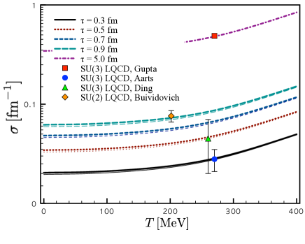
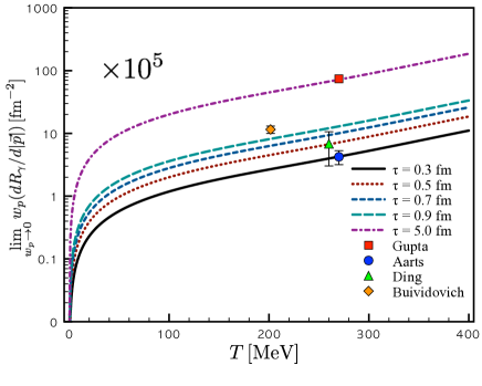
Figure 1: (Color online) Left: EC $\sigma$ as functions of temperature $T$ for different relaxation times $\tau=(0.3\sim 0.9)$ fm. The thick line indicate the case with $B_{0}=0$ ($\sigma_{\parallel}$), whereas the thin ones for $B_{0}=m^{2}_{\pi}\times 10$ ($\sigma_{\perp}$). SU($N_{c}$) LQCD estimations are taken from Refs. Gupta:2003zh (Gupta),  Aarts:2007wj (Aarts),  Ding:2010ga (Ding), and  Buividovich:2010tn (Buividovich). Right: Soft photon emission rate $\mathcal{R}_{\gamma}$ in Eq. (XXX) as functions of $T$ for different $\tau$’s in the same manner with the left panel. For all the curves in the left and right panels, I have chosen $T_{c}\approx 180$ MeV as a trial.

Finally, I would like to estimate the (differential) soft photon ($w_{p}\to 0$) emission rate from QGP for the dilepton decay rates which is related to EC as follows Gupta:2003zh ; Ding:2010ga :

$$\mathcal{R}_{\gamma}\equiv\lim_{w_{p}\to 0}w_{p}\frac{dR_{\gamma}}{d^{3}|\bm{p}|}=\frac{3\alpha_{\mathrm{EM}}}{2\pi^{2}}\sigma T.$$ (8)

The numerical results for $\mathcal{R}_{\gamma}$ in Eq. (8) are given in the right panel of figure 1 for different $\tau$, being similar to the left panel of figure 1. The LQCD results are also depicted there. It turns out that the value of $\mathcal{R}_{\gamma}$ increases rapidly near $T=0$. Beyond that, the slope of $\mathcal{R}_{\gamma}$ becomes rather flat for $T$.

IV Summary and conclusion

EC is an increasing function of $T$ and depends on $\tau$ of the quark matter. The effective quark mass was modified into a decreasing function of $T$ and $|\bm{k}|$. Typically, it turns out that $\sigma\approx(0.02\sim 0.15)\,\mathrm{fm}^{-1}$ for $T=(0\sim 400)$ MeV with the relaxation time $\tau=(0.3\sim 0.9)$ fm. Recent LQCD data are well reproduced for $\tau=(0.3\sim 0.7)\,\mathrm{fm}$ for a wide $T$ range. The effects of the external magnetic field are negligible on EC even for the very strong $\bm{B}$. Using the present numerical results obtained, EC is parameterized for $T=(0\sim 400)$ MeV with $\sigma=C_{\mathrm{EM}}(\mathcal{C}_{1}T+\mathcal{C}_{2}T^{2}+\mathcal{C}_{3}T^{3}+\cdots)$ and, in this parameterization, the coefficients for $T^{2}$ and $T^{3}$ are tiny in comparison to $\mathcal{C}_{1}$. As a result, I have $\sigma/T\approx(0.46,0.77,1.08,1.39)\,C_{\mathrm{EM}}$ for $\tau=(0.3,0.5,0.7,0.9)$ fm, respectively. These results are again well compatible with other theoretical estimations. Readers can refer to Ref. Nam:2012sg for more details of the present work. The transport coefficients for quark matter are very important physical quantities for understanding QCD at extreme conditions. In the present work, it was shown that the instanton model reproduced qualitatively well results in comparison to other theoretical results. Other transport coefficients, i.e. the shear and bulk viscosities, are under investigation within the same theoretical framework.

References

- (1) S. A. Voloshin [STAR Collaboration], Indian J. Phys. 85, 1103 (2011).
- (2) D. Kharzeev, Phys. Lett. B 633, 260 (2006).
- (3) P. V. Buividovich, M. N. Chernodub, E. V. Luschevskaya and M. I. Polikarpov, Phys. Rev. D 80, 054503 (2009).
- (4) K. Fukushima, D. E. Kharzeev and H. J. Warringa, Phys. Rev. D 78, 074033 (2008).
- (5) D. E. Kharzeev and H. U. Yee, Phys. Rev. D 83, 085007 (2011).
- (6) S. i. Nam and C. W. Kao, Phys. Rev. D 83, 096009 (2011).
- (7) H. T. Ding, A. Francis, O. Kaczmarek, F. Karsch, E. Laermann and W. Soeldner, Phys. Rev. D 83, 034504 (2011).
- (8) B. Kerbikov and M. Andreichikov, arXiv:1206.6044 [hep-ph].
- (9) D. J. Evans and G. P. Morriss, Statistical Mechanics of Non-Equilibrium Liquids, (Academic Press, London 1990).
- (10) S. Gupta, Phys. Lett. B 597, 57 (2004).
- (11) M. Harada and C. Sasaki, Phys. Rev. D 74, 114006 (2006).
- (12) E. V. Shuryak, Nucl. Phys. B203, 93 (1982).
- (13) D. Diakonov, V. Y. Petrov, Nucl. Phys. B245, 259 (1984).
- (14) D. Diakonov and A. D. Mirlin, Phys. Lett. B 203, 299 (1988).
- (15) S. i. Nam, J. Phys. G 37, 075002 (2010).
- (16) J. S. Schwinger, Phys. Rev. 82, 664 (1951).
- (17) S. i. Nam, Phys. Rev. D 80, 114025 (2009).
- (18) S. i. Nam, Phys. Rev. D 86, 033014 (2012).
- (19) Y. Aoki, Z. Fodor, S. D. Katz and K. K. Szabo, Phys. Lett. B 643, 46 (2006).
- (20) Y. Aoki, S. Borsanyi, S. Durr, Z. Fodor, S. D. Katz, S. Krieg and K. K. Szabo, JHEP 0906, 088 (2009).
- (21) S. Borsanyi et al. [Wuppertal-Budapest Collaboration], JHEP 1009, 073 (2010).
- (22) A. Bazavov et al., Phys. Rev. D 85, 054503 (2012).
- (23) Y. Maezawa, S. Aoki, S. Ejiri, T. Hatsuda, N. Ishii, K. Kanaya and N. Ukita, J. Phys. G 34, S651 (2007).
- (24) A. Ali Khan et al. [CP-PACS Collaboration], Phys. Rev. D 63, 034502 (2001).
- (25) G. Aarts, C. Allton, J. Foley, S. Hands and S. Kim, Phys. Rev. Lett. 99, 022002 (2007).
- (26) K. Tuchin, Phys. Rev. C 82, 034904 (2010) [Erratum-ibid. C 83, 039903 (2011)].
- (27) P. V. Buividovich et al., Phys. Rev. Lett. 105, 132001 (2010).
- (28) D. Fernandez-Fraile and A. Gomez Nicola, Eur. Phys. J. C 62, 37 (2009).