Target Detection and Characterization from Electromagnetic Induction Data

Abstract

The goal of this paper is to contribute to the field of nondestructive testing by eddy currents. We provide a mathematical analysis and a numerical framework for simulating the imaging of arbitrarily shaped small volume conductive inclusions from electromagnetic induction data. We derive, with proof, a small-volume expansion of the eddy current data measured away from the conductive inclusion. The formula involves two polarization tensors: one associated with the magnetic contrast and the second with the conductivity of the inclusion. Based on this new formula, we design a location search algorithm. We include in this paper a discussion on data sampling, noise reduction, and on probability of detection. We provide numerical examples that support our findings.

Mathematics Subject Classification (MSC2000): 35R30, 35B30

Keywords: eddy current, imaging, induction data, asymptotic formula, detection test, localization, characterization, Hadamard technique, measurement noise

1 Introduction

Nondestructive testing by eddy currents is a technology of choice in the assessment of the structural integrity of a variety of materials such as, for instance, aircrafts or metal beams, see [12]. It is also of interest in technologies related to safety of public arenas where a large number of people have to be screened.

We introduce in this paper a novel analysis pertaining to small-volume expansions for eddy current equations, which we then apply to developing new imaging techniques. Our mathematical analysis extends recently established results and methods for full Maxwell’s equations to the eddy current regime.

We propose a new eddy current reconstruction method relying on the assumption that the objects to be imaged are small. This present study is related to the theory of small-volume perturbations of Maxwell’s equations, see [10]. It is, however, specific to eddy currents and to the particular lengthscales relevant to that case.

We first note that in the eddy current regime a diffusion equation is used for modeling electromagnetic fields. The characteristic length is the skin depth of the conductive object to be imaged [12]. We consider the regime where the skin depth is comparable to the characteristic size of the conductive inclusion.

Using the ${\itbf E}$-formulation for the eddy current problem, we first establish energy estimates. We start from integral representation formulas for the electromagnetic fields arising in the presence of a small conductive inclusion to rigorously derive an asymptotic expansion for the magnetic part of the field. The effect of the conductive targets on the magnetic field measured away from the target is expressed in terms of two polarization tensors: one associated with the magnetic contrast (called magnetic polarization tensor) and the second with the conductivity of the target (called conductivity polarization tensor). The magnetic polarization tensor has been first introduced in [10] in the zero conductivity case while the concept of conductivity polarization tensor appears to be new.

Based on our asymptotic formula we are then able to construct a localization method for the conductive inclusion. That method involves a response matrix data. A MUSIC (which stands for MUltiple Signal Classification) imaging functional is proposed for locating the target. It uses the projection of a magnetic dipole located at the search point onto the image space of the response matrix. Once the location is found, geometric features of the inclusion may be reconstructed using a least-squares method. These geometric features together with material parameters (electric conductivity and magnetic permeability) are incorporated in the conductivity and magnetic polarization tensors. It is worth emphasizing that, as will be shown by our asymptotic expansion, the perturbations in the magnetic field due to the presence of the inclusion are complex-valued while the unperturbed field can be chosen to be real. As consequence, we only process the imaginary part of the recorded perturbations. Doing so, we do not need to know the unperturbed field with an order of accuracy higher than the order of magnitude of the perturbation. An approximation of lower order of the unperturbed field is enough.

The so called Hadamard measurement sampling technique is applied in order to reduce the impact of noise in measurements. We briefly explain some underlying basic ideas. Moreover, we provide statistical distributions for the singular values of the response matrix in the presence of measurement noise. An important strength of our analysis is that it can be applied for rectangular response matrices. Finally, we simulate our localization technique on a test example.

The paper is organized as follows. Section 2 is devoted to a variational formulation of the eddy current equations. Section 3 contains the main contributions of this paper. It provides a rigorous derivation of the effect of a small conductive inclusion on the magnetic field measured away from the inclusion. Section 4 extends MUSIC-type localization proposed in [6] to the eddy current model. Section 5 discusses the effect of noise on the inclusion detection and proposes a detection test based on the significant eigenvalues of the response matrix. Section 6 illustrates numerically on test examples our main findings in this paper. A few concluding remarks are given in the last section.

2 Eddy Current Equations

Suppose that there is an electromagnetic inclusion in $\mathbb{R}^{3}$ of the form $B_{\alpha}={\itbf z}+\alpha B$, where $B\subset\mathbb{R}^{3}$ is a bounded, smooth domain containing the origin. Let $\Gamma$ and $\Gamma_{\alpha}$ denote the boundary of $B$ and $B_{\alpha}$. Let $\mu_{0}$ denote the magnetic permeability of the free space. Let $\mu_{*}$ and $\sigma_{*}$ denote the permeability and the conductivity of the inclusion which are also assumed to be constant. We introduce the piecewise constant magnetic permeability and electric conductivity

$$\mu_{\alpha}({\itbf x})=\left\{\begin{array}[]{ll}\mu_{*}&\mbox{in $B_{\alpha}$, }\\ \vskip 6.0pt plus 2.0pt minus 2.0pt\cr\mu_{0}&\mbox{in $B^{c}_{\alpha}=\mathbb{R}^{3}\backslash\bar{B}_{\alpha},$}\end{array}\right.\ \ \ \ \sigma_{\alpha}({\itbf x})=\left\{\begin{array}[]{ll}\sigma_{*}&\mbox{in $B_{\alpha}$, }\\ \vskip 6.0pt plus 2.0pt minus 2.0pt\cr 0&\mbox{in $B_{\alpha}^{c}$.}\end{array}\right.$$

Let $({\itbf E}_{\alpha},{\itbf H}_{\alpha})$ denote the eddy current fields in the presence of the electromagnetic inclusion $B_{\alpha}$ and a source current ${\itbf J}_{0}$ located outside the inclusion. Moreover, we suppose that ${\itbf J}_{0}$ has a compact support and is divergence free: $\nabla\cdot{\itbf J}_{0}=0$ in $\mathbb{R}^{3}$. The fields ${\itbf E}_{\alpha}$ and ${\itbf H}_{\alpha}$ are the solutions of the following eddy current equations:

$$\left\{\begin{array}[]{l}{\nabla\times}{\itbf E}_{\alpha}=\mathrm{i}\omega\mu_{\alpha}{\itbf H}_{\alpha}\ \ \ \hbox{ in }\mathbb{R}^{3},\\ \vskip 6.0pt plus 2.0pt minus 2.0pt\cr{\nabla\times}{\itbf H}_{\alpha}=~{}\sigma_{\alpha}{\itbf E}_{\alpha}+{\itbf J}_{0}\ \ \ \hbox{ in }\mathbb{R}^{3},\\ \vskip 6.0pt plus 2.0pt minus 2.0pt\cr{\itbf E}_{\alpha}({\itbf x})=O(|{\itbf x}|^{-1}),\ \ {\itbf H}_{\alpha}({\itbf x})=O(|{\itbf x}|^{-1})\ \ \ \mbox{ as }|{\itbf x}|\rightarrow\infty.\end{array}\right.$$ (2.5)

By eliminating ${\itbf H}_{\alpha}$ in (2.5) we obtain the following ${\itbf E}$-formulation of the eddy current problem (2.5):

$$\left\{\begin{array}[]{l}{\nabla\times}\mu^{-1}_{\alpha}{\nabla\times}{\itbf E}_{\alpha}-\mathrm{i}\omega\sigma_{\alpha}{\itbf E}_{\alpha}=\mathrm{i}\omega{\itbf J}_{0}\ \ \ \mbox{ in }\mathbb{R}^{3},\\ \vskip 6.0pt plus 2.0pt minus 2.0pt\cr{\nabla\cdot}{\itbf E}_{\alpha}=0\ \ \ \mbox{ in }B_{\alpha}^{c},\\ \vskip 6.0pt plus 2.0pt minus 2.0pt\cr{\itbf E}_{\alpha}({\itbf x})=O(|{\itbf x}|^{-1})\ \ \ \mbox{ as }|{\itbf x}|\rightarrow\infty.\end{array}\right.$$ (2.9)

Throughout this paper, let ${\itbf u}^{\pm}$ denote the limit values of ${\itbf u}({\itbf x}\pm t{\itbf n})$ as $t\searrow 0$, where ${\itbf n}$ is the outward normal to $\Gamma_{\alpha}$, if they exist. We will use the function spaces

$${\bf X}_{\alpha}(\mathbb{R}^{3})=\left\{{\itbf u}:\frac{{\itbf u}}{\sqrt{1+|{\itbf x}|^{2}}}\in L^{2}(\mathbb{R}^{3})^{3},{\nabla\times}{\itbf u}\in L^{2}(\mathbb{R}^{3})^{3},{\nabla\cdot}{\itbf u}=0\mbox{ in }B_{\alpha}^{c}\right\},$$

and

$$\widetilde{{\bf X}}_{\alpha}(\mathbb{R}^{3})=\left\{{\itbf u}:{{\itbf u}}\in{\bf X}_{\alpha}(\mathbb{R}^{3}),\int_{\Gamma_{\alpha}}{\itbf u}^{+}\cdot{\itbf n}=0\right\},$$

and the sesquilinear form on $\widetilde{{\bf X}}_{\alpha}(\mathbb{R}^{3})\times\widetilde{{\bf X}}_{\alpha}(\mathbb{R}^{3})$

$$a_{\alpha}({\itbf E},{\itbf v})=(\mu^{-1}_{\alpha}{\nabla\times}{\itbf E},{\nabla\times}{\itbf v})_{\mathbb{R}^{3}}-\mathrm{i}\omega\sigma_{*}({\itbf E},{\itbf v})_{B_{\alpha}},$$

where $(\cdot,\cdot)_{D}$ stands for the $L^{2}$ inner product on the domain $D\subseteq\mathbb{R}^{3}$. The weak formulation of the ${\itbf E}$-formulation (2.9) is: Find ${\itbf E}_{\alpha}\in\widetilde{{\bf X}}_{\alpha}(\mathbb{R}^{3})$ such that

$$a_{\alpha}({\itbf E}_{\alpha},{\itbf v})=\mathrm{i}\omega({\itbf J}_{0},{\itbf v})_{B^{c}_{\alpha}},\ \ \ \forall{\itbf v}\in\widetilde{{\bf X}}_{\alpha}(\mathbb{R}^{3}).$$ (2.10)

The uniqueness and existence of solution of the problem (2.10) is known (cf., e.g., Ammari et al. [3] and Hiptmair [18]). Note that the constraint $\int_{\Gamma_{\alpha}}{\itbf u}^{+}\cdot{\itbf n}=0$ in $\widetilde{{\bf X}}_{\alpha}(\mathbb{R}^{3})$ only serves to enforce the uniqueness of ${\itbf E}_{\alpha}$ in $B^{c}_{\alpha}$ [18]. This is not essential for the validity of the ${\itbf E}$-formulation of the eddy current model. We have

$$a_{\alpha}({\itbf E}_{\alpha},{\itbf v})=\mathrm{i}\omega({\itbf J}_{0},{\itbf v})_{B^{c}_{\alpha}},\ \ \ \forall{\itbf v}\in{{\bf X}}_{\alpha}(\mathbb{R}^{3}).$$ (2.11)

Throughout the paper we denote by ${\itbf E}_{0}$ the unique solution of the problem

$$\left\{\begin{array}[]{l}{\nabla\times}\mu^{-1}_{0}{\nabla\times}{\itbf E}_{0}=\mathrm{i}\omega{\itbf J}_{0}\ \ \ \mbox{ in }\mathbb{R}^{3},\\ \vskip 6.0pt plus 2.0pt minus 2.0pt\cr{\nabla\cdot}{\itbf E}_{0}=0\mbox{ in }\mathbb{R}^{3},\\ \vskip 6.0pt plus 2.0pt minus 2.0pt\cr{\itbf E}_{0}({\itbf x})=O(|{\itbf x}|^{-1})\ \ \ \mbox{ as }|{\itbf x}|\rightarrow\infty.\end{array}\right.$$ (2.12)

The field ${\itbf E}_{0}$ satisfies

$$(\mu^{-1}_{0}{\nabla\times}{\itbf E}_{0},{\nabla\times}{\itbf v})_{\mathbb{R}^{3}}=\mathrm{i}\omega({\itbf J}_{0},{\itbf v})_{\mathbb{R}^{3}},\ \ \ \forall{\itbf v}\in{\bf H}_{-1}(\mathbf{curl};\mathbb{R}^{3}),$$ (2.13)

where $\displaystyle{\bf H}_{-1}(\mathbf{curl};\mathbb{R}^{3})=\Big{\{}{\itbf u}:\frac{{\itbf u}}{\sqrt{1+|{\itbf x}|^{2}}}\in L^{2}(\mathbb{R}^{3})^{3},{\nabla\times}{\itbf u}\in L^{2}(\mathbb{R}^{3})^{3}\Big{\}}$.

3 Derivation of the Asymptotic Formulas

In this section we will derive the asymptotic formula for ${\itbf H}_{\alpha}$ when the inclusion is small. Let $k=\omega\mu_{0}\sigma_{*}$. We are interested in the asymptotic regime when $\alpha\rightarrow 0$ and

$$\nu=k\alpha^{2}$$ (3.1)

is of order one. Moreover, we assume that $\mu_{*}$ and $\mu_{0}$ are of the same order.

In eddy current testing the wave equation is converted into the diffusion equation, where the characteristic length is the skin depth $\delta$, given by $\delta=\sqrt{2/k}$. Hence, in the regime $\nu=O(1)$, the skin depth $\delta$ is of order of the characteristic size $\alpha$ of the inclusion.

We will always denote by $C$ a generic constant which depends possibly on $\mu_{*}/\mu_{0}$, the upper bound of $\omega\mu_{0}\sigma_{*}\alpha^{2}$, the domain $B$, but is independent of $\omega,\sigma_{*},\mu_{0},\mu_{*}$. Let $\mu_{r}=\mu_{*}/\mu_{0}.$

3.1 Energy Estimates

We start with the following estimate.

Lemma 3.1

There exists a constant $C$ such that

$$\|{\nabla\times}({\itbf E}_{\alpha}-{\itbf E}_{0})\|_{L^{2}(\mathbb{R}^{3})}+\sqrt{k}\|{\itbf E}_{\alpha}-{\itbf E}_{0}\|_{L^{2}(B_{\alpha})}\leq C\alpha^{3/2}(\sqrt{k}\|{\itbf E}_{0}\|_{L^{\infty}(B_{\alpha})}+\|{\nabla\times}{\itbf E}_{0}\|_{L^{\infty}(B_{\alpha})}).$$

Proof. By (2.11) and (2.13), we know that

$$(\mu^{-1}_{\alpha}{\nabla\times}({\itbf E}_{\alpha}-{\itbf E}_{0}),{\nabla\times}{\itbf v})_{\mathbb{R}^{3}}-\mathrm{i}\omega(\sigma_{\alpha}({\itbf E}_{\alpha}-{\itbf E}_{0}),{\itbf v})_{B_{\alpha}}$$

$$\qquad=(\mu_{0}^{-1}-\mu_{*}^{-1})({\nabla\times}{\itbf E}_{0},{\nabla\times}{\itbf v})_{B_{\alpha}}+\mathrm{i}\omega(\sigma_{\alpha}{\itbf E}_{0},{\itbf v})_{B_{\alpha}},\ \ \ \forall{\itbf v}\in{\bf X}_{\alpha}(\mathbb{R}^{3}).$$ (3.2)

Since

$$|({\nabla\times}{\itbf E}_{0},{\nabla\times}{\itbf v})_{B_{\alpha}}|\leq C\alpha^{3/2}\|{\nabla\times}{\itbf E}_{0}\|_{L^{\infty}(B_{\alpha})}\|{\nabla\times}{\itbf v}\|_{L^{2}(B_{\alpha})}$$

and

$$|(\sigma_{\alpha}{\itbf E}_{0},{\itbf v})|\leq C\alpha^{3/2}\sigma_{*}\|{\itbf E}_{0}\|_{L^{\infty}(B_{\alpha})}\|{\itbf v}\|_{L^{2}(B_{\alpha})},$$

by taking ${\itbf v}={\itbf E}_{\alpha}-{\itbf E}_{0}\in{\bf X}_{\alpha}(\mathbb{R}^{3})$ in (3.1) and multiplying the obtained equation by $\mu_{0}$ we have that

$$\mu_{r}^{-1}\|{\nabla\times}({\itbf E}_{\alpha}-{\itbf E}_{0})\|_{L^{2}(\mathbb{R}^{3})}^{2}+k\|{\itbf E}_{\alpha}-{\itbf E}_{0}\|_{L^{2}(B_{\alpha})}^{2}$$

$$\leq C\alpha^{3/2}\left(\|{\nabla\times}{\itbf E}_{0}\|_{L^{\infty}(B_{\alpha})}\|{\nabla\times}({\itbf E}_{\alpha}-{\itbf E}_{0})\|_{L^{2}(B_{\alpha})}+k\|{\itbf E}_{0}\|_{L^{\infty}(B_{\alpha})}\|{\itbf E}_{\alpha}-{\itbf E}_{0}\|_{L^{2}(B_{\alpha})}\right).$$

This completes the proof. $\Box$

Let $H^{1}(B_{\alpha})=\{\varphi\in L^{2}(B_{\alpha}),\nabla\varphi\in L^{2}(B_{\alpha})^{3}\}$. Let $\phi_{0}\in H^{1}(B_{\alpha})$ be the solution of the problem

$$-\Delta\phi_{0}=-\nabla\cdot{\itbf F}\mbox{ in }B_{\alpha},\ \ \ -\partial_{\itbf n}\phi_{0}=({\itbf E}_{0}({\itbf x})-{\itbf F}({\itbf x}))\cdot{\itbf n}\mbox{ on }\Gamma_{\alpha},\ \ \ \int_{B_{\alpha}}\phi_{0}\,d{\itbf x}=0,$$ (3.3)

where

$${\itbf F}({\itbf x})=\frac{1}{2}[\nabla_{\itbf z}\times{\itbf E}_{0}({\itbf z})]\times({\itbf x}-{\itbf z})+\frac{1}{3}[{\bf D}_{\itbf z}(\nabla_{\itbf z}\times{\itbf E}_{0})({\itbf z})]({\itbf x}-{\itbf z})\times({\itbf x}-{\itbf z}).$$ (3.4)

Here $[{\bf D}_{\itbf z}(\nabla_{\itbf z}\times{\itbf E}_{0})({\itbf z})]_{ij}=\partial_{z_{i}}(\nabla_{\itbf z}\times{\itbf E}_{0}({\itbf z}))_{j}$ is the $(i,j)$-th element of the gradient matrix ${\bf D}_{\itbf z}(\nabla_{\itbf z}\times{\itbf E}_{0})({\itbf z})$ of $\nabla_{\itbf z}\times{\itbf E}_{0}({\itbf z})$. Let ${\rm tr}$ denote the trace. Since ${\rm tr}[{\bf D}(\nabla\times{\itbf E}_{0})]=\nabla\cdot(\nabla\times{\itbf E}_{0})=0$, we know that

$$\nabla\times{\itbf F}({\itbf x})=\nabla_{\itbf z}\times{\itbf E}_{0}({\itbf z})+[{\bf D}_{\itbf z}(\nabla_{\itbf z}\times{\itbf E}_{0})({\itbf z})]({\itbf x}-{\itbf z}).$$ (3.5)

Note that since ${\itbf E}_{0}$ is smooth in $\bar{B}_{\alpha}$ we have

$$\|\nabla\times{\itbf E}_{0}-\nabla\times{\itbf F}\|_{L^{\infty}(B_{\alpha})}\leq C\alpha^{2}\|\nabla\times{\itbf E}_{0}\|_{W^{2,\infty}(B_{\alpha})}.$$ (3.6)

Denote by $\displaystyle{\itbf H}_{0}=(\mathrm{i}\omega\mu_{0})^{-1}{\nabla\times}{\itbf E}_{0}$ and introduce ${\itbf w}\in\widetilde{{\bf X}}_{\alpha}(\mathbb{R}^{3})$ as the solution of the problem

$$a_{\alpha}({\itbf w},{\itbf v}) = \mathrm{i}\omega\mu_{0}(\mu_{0}^{-1}-\mu_{*}^{-1})({\itbf H}_{0}({\itbf z})+{\bf D}{\itbf H}_{0}({\itbf z})({\itbf x}-{\itbf z}),{\nabla\times}{\itbf v})_{B_{\alpha}}$$ (3.7)

$$+\mathrm{i}\omega(\sigma_{\alpha}{\itbf F},{\itbf v})_{B_{\alpha}},\qquad\forall{\itbf v}\in\widetilde{{\bf X}}_{\alpha}.$$

The following lemma provides a higher-order correction of the error estimate in Lemma 3.1.

Lemma 3.2

Let ${\itbf w}$ be defined by (3.7). There exists a constant $C$ such that

$$\|{\nabla\times}({\itbf E}_{\alpha}-{\itbf E}_{0}-{\itbf w})\|_{L^{2}(\mathbb{R}^{3})}\leq C\alpha^{7/2}(|1-\mu_{r}^{-1}|+\nu)\|\nabla\times{\itbf E}_{0}\|_{W^{2,\infty}(B_{\alpha})},$$ (3.8)

$$\|{\itbf E}_{\alpha}-{\itbf E}_{0}-\nabla\phi_{0}-{\itbf w}\|_{L^{2}(B_{\alpha})}\leq C\alpha^{9/2}(|1-\mu_{r}^{-1}|+\nu)\|\nabla\times{\itbf E}_{0}\|_{W^{2,\infty}(B_{\alpha})},$$ (3.9)

where $\nu$ is given by (3.1).

Proof. First we set $\psi\in H^{1}(B_{\alpha})$ and $g$ be such that $g=\psi$ on $\Gamma_{\alpha}$, $\Delta g=0$ in $B_{\alpha}^{c}$, and $g=O(|{\itbf x}|^{-1})$ at infinity. Let

$${\itbf v}:=\left\{\begin{array}[]{l}\nabla\psi\quad\mbox{in }B_{\alpha},\\ \vskip 6.0pt plus 2.0pt minus 2.0pt\cr\nabla g\quad\mbox{in }B_{\alpha}^{c}.\end{array}\right.$$

Since ${\itbf v}\in{\bf X}_{\alpha}$, it follows from (2.11) that

$$\mathrm{i}\omega(\sigma_{\alpha}{\itbf E}_{\alpha},\nabla\psi)_{B_{\alpha}}=0,\ \ \ \forall\psi\in H^{1}(B_{\alpha}).$$

This yields ${\nabla\cdot}{\itbf E}_{\alpha}=0$ in $B_{\alpha}$ and ${\itbf E}_{\alpha}^{-}\cdot{\itbf n}=0$ on $\Gamma_{\alpha}$.

Similarly, we can show from (3.7) that ${\itbf w}^{-}\cdot{\itbf n}=-{\itbf F}({\itbf x})\cdot{\itbf n}$ on $\Gamma_{\alpha}$ and ${\nabla\cdot}{\itbf w}=-\nabla\cdot{\itbf F}$ in $B_{\alpha}$. From (3.3) we also know that ${\nabla\cdot}({\itbf E}_{0}+\nabla\phi_{0})=\nabla\cdot{\itbf F}$ in $B_{\alpha}$ and $({\itbf E}_{0}+\nabla\phi_{0})^{-}\cdot{\itbf n}={\itbf F}({\itbf x})\cdot{\itbf n}$ on $\Gamma_{\alpha}$. Thus

$$\nabla\cdot\left({\itbf E}_{\alpha}-{\itbf E}_{0}-\nabla\phi_{0}-{\itbf w}\right)=0\ \ \mbox{in }B_{\alpha},\ \ \ \ \left({\itbf E}_{\alpha}-{\itbf E}_{0}-\nabla\phi_{0}-{\itbf w}\right)^{-}\cdot{\itbf n}=0\ \ \mbox{on }\Gamma_{\alpha},$$

which implies by scaling argument and the embedding theorem that

$$\|{\itbf E}_{\alpha}-{\itbf E}_{0}-\nabla\phi_{0}-{\itbf w}\|_{L^{2}(B_{\alpha})} \leq C\alpha\|\nabla\times\left({\itbf E}_{\alpha}-{\itbf E}_{0}-\nabla\phi_{0}-{\itbf w}\right)\|_{L^{2}(B_{\alpha})}$$

$$= C\alpha\|\nabla\times\left({\itbf E}_{\alpha}-{\itbf E}_{0}-{\itbf w}\right)\|_{L^{2}(B_{\alpha})},$$

for some constant $C$ independent of $\alpha$ and $\sigma_{*}$. Therefore, (3.9) follows from (3.8).

To show (3.8), we define $\tilde{\phi}_{0}$ as the solution of the exterior problem

$$-\Delta\tilde{\phi}_{0}=0\mbox{ in }B^{c}_{\alpha},\ \ \ \tilde{\phi}_{0}=\phi_{0}\mbox{ on }\Gamma_{\alpha},\ \ \ \tilde{\phi}_{0}\rightarrow 0\mbox{ as }|{\itbf x}|\rightarrow\infty.$$

The existence of $\tilde{\phi}_{0}$ in $\displaystyle W^{1,-1}(B^{c}_{\alpha})=\Big{\{}\varphi:\frac{\varphi}{\sqrt{1+|{\itbf x}|^{2}}}\in L^{2}(B_{\alpha}^{c}),\nabla\varphi\in L^{2}(B_{\alpha}^{c})^{3}\Big{\}}$ is known (cf., e.g., Nédélec [21]).

Define ${\bm{\Phi}}_{0}=\nabla\phi_{0}$ in $B_{\alpha}$, ${\bm{\Phi}}_{0}=\nabla\tilde{\phi}_{0}$ in $B_{\alpha}^{c}$, then ${\bm{\Phi}}_{0}\in{\bf X}_{\alpha}(\mathbb{R}^{3})$. It follows from (3.1) and (3.7) that for all ${\itbf v}\in{\bf X}_{\alpha}(\mathbb{R}^{3})$

$$(\mu^{-1}_{\alpha}{\nabla\times}({\itbf E}_{\alpha}-{\itbf E}_{0}-{\bm{\Phi}}_{0}-{\itbf w}),{\nabla\times}{\itbf v})_{\mathbb{R}^{3}}-\mathrm{i}\omega(\sigma_{\alpha}({\itbf E}_{\alpha}-{\itbf E}_{0}-{\bm{\Phi}}_{0}-{\itbf w}),{\itbf v})_{B_{\alpha}}$$

$$=\mathrm{i}\omega\mu_{0}(\mu_{0}^{-1}-\mu_{*}^{-1})({\itbf H}_{0}-{\itbf H}_{0}({\itbf z})-{\bf D}{\itbf H}_{0}({\itbf z})({\itbf x}-{\itbf z}),{\nabla\times}{\itbf v})_{B_{\alpha}}+\mathrm{i}\omega(\sigma_{\alpha}({\itbf E}_{0}+{\bm{\Phi}}_{0}-{\itbf F}),{\itbf v})_{B_{\alpha}}.$$

By multiplying the above equation by $\mu_{0}$ we have then

$$(\mu_{0}\mu_{\alpha}^{-1}{\nabla\times}({\itbf E}_{\alpha}-{\itbf E}_{0}-{\bm{\Phi}}_{0}-{\itbf w}),{\nabla\times}{\itbf v})_{\mathbb{R}^{3}}-\mathrm{i}k({\itbf E}_{\alpha}-{\itbf E}_{0}-{\bm{\Phi}}_{0}-{\itbf w},{\itbf v})_{B_{\alpha}}$$

$$=\mathrm{i}\omega\mu_{0}(1-\mu_{r}^{-1})({\itbf H}_{0}-{\itbf H}_{0}({\itbf z})-{\bf D}{\itbf H}_{0}({\itbf z})({\itbf x}-{\itbf z}),{\nabla\times}{\itbf v})_{B_{\alpha}}+\mathrm{i}k({\itbf E}_{0}+{\bm{\Phi}}_{0}-{\itbf F},{\itbf v})_{B_{\alpha}}.$$ (3.10)

It is easy to check that

$$|\mathrm{i}\omega\mu_{0}({\itbf H}_{0}-{\itbf H}_{0}({\itbf z})-{\bf D}{\itbf H}_{0}({\itbf z})({\itbf x}-{\itbf z}),{\nabla\times}{\itbf v})_{B_{\alpha}}| \leq C\alpha^{7/2}\|\mathrm{i}\omega\mu_{0}{\itbf H}_{0}\|_{W^{2,\infty}(B_{\alpha})}\|{\nabla\times}{\itbf v}\|_{L^{2}(B_{\alpha})}$$

$$= C\alpha^{7/2}\|\nabla\times{\itbf E}_{0}\|_{W^{2,\infty}(B_{\alpha})}\|{\nabla\times}{\itbf v}\|_{L^{2}(B_{\alpha})}.$$

Now taking ${\itbf v}={\itbf E}_{\alpha}-{\itbf E}_{0}-{\bm{\Phi}}_{0}-{\itbf w}\in{\bf X}_{\alpha}(\mathbb{R}^{3})$ in (3.1), since $\nabla\times{\bm{\Phi}}_{0}=0$ in $\mathbb{R}^{3}$ and ${\bm{\Phi}}_{0}=\nabla\phi_{0}$ in $B_{\alpha}$, we obtain that

$$\|{\nabla\times}({\itbf E}_{\alpha}-{\itbf E}_{0}-{\itbf w})\|^{2}_{L^{2}(\mathbb{R}^{3})}+k\|{\itbf E}_{\alpha}-{\itbf E}_{0}-\nabla\phi_{0}-{\itbf w}\|^{2}_{L^{2}(B_{\alpha})}$$

$$\leq C\alpha^{7/2}|1-\mu_{r}^{-1}|\|\nabla\times{\itbf E}_{0}\|_{W^{2,\infty}(B_{\alpha})}\|{\nabla\times}{\itbf v}\|_{L^{2}(B_{\alpha})}+k\|{\itbf E}_{0}-{\itbf F}+\nabla\phi_{0}\|_{L^{2}(B_{\alpha})}\|{\itbf v}\|_{L^{2}(B_{\alpha})}$$

$$\leq C\alpha^{7/2}(|1-\mu_{r}^{-1}|+\nu)\|\nabla\times{\itbf E}_{0}\|_{W^{2,\infty}(B_{\alpha})}\|{\nabla\times}{\itbf v}\|_{L^{2}(B_{\alpha})}.$$

Here, we have used

$$\|{\itbf E}_{0}-{\itbf F}+\nabla\phi_{0}\|_{L^{2}(B_{\alpha})}\leq C\alpha\|\nabla\times({\itbf E}_{0}-{\itbf F})\|_{L^{2}(B_{\alpha})}\leq C\alpha^{9/2}\|\nabla\times{\itbf E}_{0}\|_{W^{2,\infty}(B_{\alpha})}$$ (3.11)

and $\|{\itbf v}\|_{L^{2}(B_{\alpha})}\leq C\alpha\|\nabla\times{\itbf v}\|_{L^{2}(B_{\alpha})}$, since ${\itbf E}_{0}-{\itbf F}+\nabla\phi_{0}$ and ${\itbf v}$ are divergence free in $B_{\alpha}$ and have vanishing normal traces on $\Gamma_{\alpha}$. This shows (3.8) and completes the proof. $\Box$

We note that ${\bf D}{\itbf H}_{0}({\itbf z})$ is symmetric since $\nabla\times{\itbf H}_{0}({\itbf z})=0$. Hence, by Green’s formula,

$$\displaystyle(\mu_{0}^{-1}-\mu_{*}^{-1})({\itbf H}_{0}({\itbf z})+{\bf D}{\itbf H}_{0}({\itbf z})({\itbf x}-{\itbf z}),{\nabla\times}{\itbf v})_{B_{\alpha}}$$

$$= \displaystyle(\mu_{0}^{-1}-\mu_{*}^{-1})\int_{\Gamma_{\alpha}}(({\itbf H}_{0}({\itbf z})+{\bf D}{\itbf H}_{0}({\itbf z})({\itbf x}-{\itbf z}))\times{\itbf n})\cdot{\itbf v}d{\itbf x}$$

$$= \displaystyle\int_{\Gamma_{\alpha}}[\mu_{\alpha}^{-1}({\itbf H}_{0}({\itbf z})+{\bf D}{\itbf H}_{0}({\itbf z})({\itbf x}-{\itbf z}))\times{\itbf n}]_{\Gamma_{\alpha}}\cdot{\itbf v}d{\itbf x},$$

where $[\cdot]_{\Gamma_{\alpha}}$ stands for the jump of the function across $\Gamma$. Let $\hat{\itbf w}({\bm{\xi}})={\itbf w}({\itbf z}+\alpha{\bm{\xi}})$, we know from (3.7) that, $\forall{\itbf v}\in\widetilde{{\bf X}}_{1}(\mathbb{R}^{3})$,

$$\displaystyle(\mu^{-1}{\nabla\times}\hat{\itbf w},{\nabla\times}{\itbf v})_{\mathbb{R}^{3}}-\mathrm{i}\omega\alpha^{2}(\sigma\hat{\itbf w},{\itbf v})_{B} = \displaystyle\mathrm{i}\alpha\omega\mu_{0}\int_{\Gamma}[\mu^{-1}({\itbf H}_{0}({\itbf z})+\alpha{\bf D}{\itbf H}_{0}({\itbf z})\bm{\xi})\times{\itbf n}]_{\Gamma}\cdot{\itbf v}d{\bm{\xi}}$$

$$\displaystyle+\mathrm{i}\omega\alpha^{2}(\sigma{\itbf F}({\itbf z}+\alpha\bm{\xi}),{\itbf v})_{B},$$

where $\mu({\bm{\xi}})=\mu_{*}$ if ${\bm{\xi}}\in B$, $\mu({\bm{\xi}})=\mu_{0}$ if ${\bm{\xi}}\in B^{c}$ and $\sigma({\bm{\xi}})=\sigma_{*}$ if ${\bm{\xi}}\in B$, $\sigma({\bm{\xi}})=0$ if ${\bm{\xi}}\in B^{c}$.

This motivates us to introduce the solution ${\itbf w}_{0}({\bm{\xi}})$ of the interface problem

$$\left\{\begin{array}[]{l}\nabla_{\bm{\xi}}\times\mu^{-1}\nabla_{\bm{\xi}}\times{\itbf w}_{0}-\mathrm{i}\omega\sigma\alpha^{2}{\itbf w}_{0}=\mathrm{i}\omega\sigma\alpha^{2}\left[\alpha^{-1}{\itbf F}({\itbf z}+\alpha\bm{\xi})\right]\mbox{ in }B\cup B^{c},\\ \vskip 6.0pt plus 2.0pt minus 2.0pt\cr\nabla_{\bm{\xi}}\cdot{\itbf w}_{0}=0\mbox{ in }B^{c},\\ \vskip 6.0pt plus 2.0pt minus 2.0pt\cr\mbox{[}{\itbf w}_{0}\times{\itbf n}]_{\Gamma}=0,\ \ \ [\mu^{-1}\nabla_{\bm{\xi}}\times{\itbf w}_{0}\times{\itbf n}]_{\Gamma}=-\mathrm{i}\omega(1-\mu_{r}^{-1})({\itbf H}_{0}({\itbf z})+\alpha{\bf D}{\itbf H}_{0}({\itbf z})\bm{\xi})\times{\itbf n}\mbox{ on }\Gamma,\\ \vskip 6.0pt plus 2.0pt minus 2.0pt\cr{\itbf w}_{0}(\bm{\xi})=O(|\bm{\xi}|^{-1})\mbox{ as }|\bm{\xi}|\rightarrow\infty.\end{array}\right.$$ (3.12)

It is easy to check that $\displaystyle{\itbf w}({\itbf x})=\alpha{\itbf w}_{0}\Big{(}\frac{{\itbf x}-{\itbf z}}{\alpha}\Big{)}$.

The following theorem which is the main result of this section now follows directly from Lemma 3.2.

Theorem 3.1

There exists a constant $C$ such that

$$\Big{\|}{\nabla\times}\Big{(}{\itbf E}_{\alpha}-{\itbf E}_{0}-\alpha{\itbf w}_{0}(\frac{{\itbf x}-{\itbf z}}{\alpha})\Big{)}\Big{\|}_{L^{2}(B_{\alpha})}\leq C\alpha^{7/2}(|1-\mu_{r}^{-1}|+\nu)\|\nabla\times{\itbf E}_{0}\|_{W^{2,\infty}(B_{\alpha})},$$

$$\Big{\|}{\itbf E}_{\alpha}-{\itbf E}_{0}-\nabla\phi_{0}-\alpha{\itbf w}_{0}\Big{(}\frac{{\itbf x}-{\itbf z}}{\alpha}\Big{)}\Big{\|}_{L^{2}(B_{\alpha})}\leq C\alpha^{9/2}(|1-\mu_{r}^{-1}|+\nu)\|\nabla\times{\itbf E}_{0}\|_{W^{2,\infty}(B_{\alpha})}.$$

To conclude this section we remark that

$$\alpha^{-1}{\itbf F}({\itbf z}+\alpha\bm{\xi}) = \mathrm{i}\omega\mu_{0}\left(\frac{1}{2}\,{\itbf H}_{0}({\itbf z})\times\bm{\xi}+\frac{\alpha}{3}\,{\bf D}{\itbf H}_{0}({\itbf z})\bm{\xi}\times\bm{\xi}\right)$$ (3.13)

$$= \mathrm{i}\omega\mu_{0}\left(\frac{1}{2}\,\sum^{3}_{i=1}{\itbf H}_{0}({\itbf z})_{i}{\itbf e}_{i}\times\bm{\xi}+\frac{\alpha}{3}\,\sum^{3}_{i,j=1}{\bf D}{\itbf H}_{0}({\itbf z})_{ij}{\itbf e}_{i}{\itbf e}_{j}^{T}\bm{\xi}\times\bm{\xi}\right),$$

where ${\bf D}{\itbf H}_{0}({\itbf z})_{ij}$ is the $(i,j)$-th element of the matrix ${\bf D}{\itbf H}_{0}({\itbf z})$ and $T$ denotes the transpose. Thus

$${\itbf w}_{0}({\bm{\xi}})=\mathrm{i}\omega\mu_{0}\left(\frac{1}{2}\sum^{3}_{i=1}{\itbf H}_{0}({\itbf z})_{i}{\bm{\theta}}_{i}({\bm{\xi}})+\frac{\alpha}{3}\,\sum^{3}_{i,j=1}{\bf D}{\itbf H}_{0}({\itbf z})_{ij}\bm{\Psi}_{ij}(\bm{\xi})\right),$$ (3.14)

where ${\bm{\theta}}_{i}({\bm{\xi}})$ is the solution of the following interface problem

$$\left\{\begin{array}[]{l}\nabla_{\bm{\xi}}\times\mu^{-1}\nabla_{\bm{\xi}}\times{\bm{\theta}}_{i}-\mathrm{i}\omega\sigma\alpha^{2}{\bm{\theta}}_{i}=\displaystyle\mathrm{i}\omega\sigma\alpha^{2}{\itbf e}_{i}\times\bm{\xi}\mbox{ in }B\cup B^{c},\\ \vskip 6.0pt plus 2.0pt minus 2.0pt\cr\nabla_{\bm{\xi}}\cdot{\bm{\theta}}_{i}=0\mbox{ in }B^{c},\\ \vskip 6.0pt plus 2.0pt minus 2.0pt\cr\mbox{[}{\bm{\theta}}_{i}\times{\itbf n}]_{\Gamma}=0,\ \ [\mu^{-1}\nabla_{\bm{\xi}}\times{\bm{\theta}}_{i}\times{\itbf n}]_{\Gamma}=-2[\mu^{-1}]_{\Gamma}{\itbf e}_{i}\times{\itbf n}\mbox{ on }{\Gamma},\\ \vskip 6.0pt plus 2.0pt minus 2.0pt\cr{\bm{\theta}}_{i}({\bm{\xi}})=O(|\bm{\xi}|^{-1})\mbox{ as }|{\bm{\xi}}|\rightarrow\infty,\end{array}\right.$$ (3.15)

and ${\bm{\Psi}}_{ij}({\bm{\xi}})$ is the solution of

$$\left\{\begin{array}[]{l}\nabla_{\bm{\xi}}\times\mu^{-1}\nabla_{\bm{\xi}}\times{\bm{\Psi}}_{ij}-\mathrm{i}\omega\sigma\alpha^{2}{\bm{\Psi}}_{ij}=\mathrm{i}\omega\sigma\alpha^{2}\xi_{j}{\itbf e}_{i}\times\bm{\xi}\mbox{ in }B\cup B^{c},\\ \vskip 6.0pt plus 2.0pt minus 2.0pt\cr\nabla_{\bm{\xi}}\cdot{\bm{\Psi}}_{ij}=0\mbox{ in }B^{c},\\ \vskip 6.0pt plus 2.0pt minus 2.0pt\cr\mbox{[}{\bm{\Psi}}_{ij}\times{\itbf n}]_{\Gamma}=0,\ \ [\mu^{-1}\nabla_{\bm{\xi}}\times{\bm{\Psi}}_{ij}\times{\itbf n}]_{\Gamma}=-3[\mu^{-1}]_{\Gamma}\xi_{j}{\itbf e}_{i}\times{\itbf n}\mbox{ on }{\Gamma},\\ \vskip 6.0pt plus 2.0pt minus 2.0pt\cr{\bm{\Psi}}_{ij}({\bm{\xi}})=O(|\bm{\xi}|^{-1})\mbox{ as }|{\bm{\xi}}|\rightarrow\infty.\end{array}\right.$$ (3.16)

Here ${\itbf e}_{i}$ is the unit vector in the $x_{i}$ direction. It is worth emphasizing that since $\nu=O(1)$, ${\bm{\theta}}_{i}$ and ${\bm{\Psi}}_{ij}$ are uniformly bounded in ${\bf X}_{1}(\mathbb{R}^{3})$.

We impose $\nabla\cdot\bm{\theta}_{i}=0$ outside $B$ to make the solution $\bm{\theta}_{i}$ unique outside $B$. In this case by [3, Proposition 3.1] we can show that $\bm{\theta}_{i}=O(|\bm{\xi}|^{-2})$ and $\nabla\times\bm{\theta}_{i}=O(|\bm{\xi}|^{-3})$ as $|\bm{\xi}|\to\infty$, which implies by integrating (3.15) over $B$ that

$$\mathrm{i}\omega\sigma_{*}\alpha^{2}\int_{B}(\bm{\theta}_{i}+{\itbf{e}_{i}}\times\bm{\xi})d\bm{\xi} = \int_{\partial B}{\itbf n}\times\mu^{-1}\nabla\times\bm{\theta}_{i}d\bm{\xi}$$

$$= \int_{\partial B_{R}}{\itbf n}\times\mu^{-1}\nabla\times\bm{\theta}_{i}d\bm{\xi}$$

$$\to 0\ \ \mbox{as }R\to+\infty,$$

where $B_{R}$ is a ball of radius $R$ so that $B\subset B_{R}$. Thus we obtain

$$\int_{B}(\bm{\theta}_{i}+{\itbf e}_{i}\times\bm{\xi})d\,\bm{\xi}=0.$$ (3.17)

Similarly, by imposing $\nabla\cdot\bm{\Psi}_{ij}=0$ outside $B$ we know that $\nabla\times\bm{\Psi}_{ij}=O(|\bm{\xi}|^{-3})$. Moreover, integrating (3.16) over $B$ and using similar argument leading to (3.17) together with the symmetry of ${\bf D}{\itbf H}_{0}({\itbf z})$ yields

$$\displaystyle\sum_{i,j=1}^{3}{\bf D}{\itbf H}_{0}({\itbf z})_{ij}\int_{B}(\bm{\Psi}_{ij}+\xi_{j}{\itbf{e}_{i}}\times\bm{\xi})d\bm{\xi}=0.$$ (3.18)

3.2 Integral Representation Formulas

The integral representation is similar to the Stratton-Chu formula for time-harmonic Maxwell equations (cf., e.g., Nédélec [21]).

Lemma 3.3

Let $D$ be a bounded domain in $\mathbb{R}^{3}$ with Lipschitz boundary $\Gamma_{D}$ whose unit outer normal is ${\itbf n}$. For any ${\itbf E}\in\mathbf{H}_{-1}(\mathbf{curl};\mathbb{R}^{3}\backslash\bar{D})$ satisfying ${\nabla\times}{\nabla\times}{\itbf E}=0,{\nabla\cdot}{\itbf E}=0$ in $\mathbb{R}^{3}\backslash\bar{D}$, we have, for any ${\itbf x}\in\mathbb{R}^{3}\backslash\bar{D}$,

$${\itbf E}({\itbf x}) = -\nabla_{\itbf x}\times\int_{\Gamma_{D}}({\itbf E}({\itbf y})\times{\itbf n})G({\itbf x},{\itbf y})d{\itbf y}-\int_{\Gamma_{D}}(\nabla_{\itbf y}\times{\itbf E}({\itbf y})\times{\itbf n})G({\itbf x},{\itbf y})d{\itbf y}$$

$$-\nabla_{\itbf x}\int_{\Gamma_{D}}({\itbf E}({\itbf y})\cdot{\itbf n})G({\itbf x},{\itbf y})d{\itbf y},$$

where $G({\itbf x},{\itbf y})=\frac{1}{4\pi|{\itbf x}-{\itbf y}|}$ is the fundamental solution of the Laplace equation.

Proof. For the sake of completeness we give a sketch of proof. Since ${\itbf E}\in\mathbf{H}_{-1}(\mathbf{curl};\mathbb{R}^{3}\backslash\bar{D})$, for any ${\itbf F}$ such that ${\itbf F}({\itbf y})=O(|{\itbf y}|^{-1})$ and ${\bf D}{\itbf F}({\itbf y})=O(|{\itbf y}|^{-2})$ as $|{\itbf y}|\to\infty$, we can obtain by integrating by parts, the conditions $\nabla\times\nabla\times{\itbf E}=0,\nabla\cdot{\itbf E}=0$ in $\mathbb{R}^{3}\backslash\bar{D}$, that

$$({\itbf E},-\Delta{\itbf F})_{\mathbb{R}^{3}\backslash\bar{D}} = ({\itbf E},{\nabla\times}{\nabla\times}{\itbf F}-\nabla{\nabla\cdot}{\itbf F})_{\mathbb{R}^{3}\backslash\bar{D}}\ \ \ \ \$$

$$= -\int_{\Gamma_{D}}({\itbf E}\times{\itbf n})\cdot{\nabla\times}{\itbf F}d{\itbf y}-\int_{\Gamma_{D}}{\nabla\times}{\itbf E}\times{\itbf n}\cdot{\itbf F}d{\itbf y}+\int_{\Gamma_{D}}({\itbf E}\cdot{\itbf n}){\nabla\cdot}{\itbf F}d{\itbf y}.$$

Now for ${\itbf x}\in\mathbb{R}^{3}\backslash\bar{D}$ and $j\in\{1,2,3\}$, we choose ${\itbf F}({\itbf y})=G({\itbf x},{\itbf y}){\itbf e}_{j}$ and thus $-\Delta_{\itbf y}{\itbf F}=\delta({\itbf x},{\itbf y}){\itbf e}_{j}$, where $\delta({\itbf x},\cdot)$ is the Dirac mass at ${\itbf x}$. Then we have

$${\itbf E}_{j}({\itbf x}) = -\int_{\Gamma_{D}}({\itbf E}({\itbf y})\times{\itbf n})\cdot\nabla_{\itbf y}\times(G({\itbf x},{\itbf y}){\itbf e}_{j})d{\itbf y}-\int_{\Gamma_{D}}(\nabla_{\itbf y}\times{\itbf E}({\itbf y})\times{\itbf n})_{j}G({\itbf x},{\itbf y})d{\itbf y}$$

$$+\int_{\Gamma_{D}}({\itbf E}({\itbf y})\cdot{\itbf n})\frac{\partial G({\itbf x},{\itbf y})}{\partial y_{j}}d{\itbf y}$$

$$= -\left(\nabla_{\itbf x}\times\int_{\Gamma_{D}}({\itbf E}({\itbf y})\times{\itbf n})G({\itbf x},{\itbf y})d{\itbf y}\right)_{j}-\int_{\Gamma_{D}}(\nabla_{\itbf y}\times{\itbf E}({\itbf y})\times{\itbf n})_{j}G({\itbf x},{\itbf y})d{\itbf y}$$

$$-\frac{\partial}{\partial x_{j}}\int_{\Gamma_{D}}({\itbf E}({\itbf y})\cdot{\itbf n})G({\itbf x},{\itbf y})d{\itbf y},$$

where we have used the fact that

$$({\itbf E}({\itbf y})\times{\itbf n})\cdot\nabla_{\itbf x}\times(G({\itbf x},{\itbf y}){\itbf e}_{j})=-(\nabla_{\itbf x}\times(G({\itbf x},{\itbf y}){\itbf E}({\itbf y})\times{\itbf n}))_{j}.$$

This completes the proof. $\Box$

The following lemma will be useful in deriving the asymptotic formula in next subsection. Recall that $\displaystyle{\itbf H}_{\alpha}=\frac{1}{\mathrm{i}\omega\mu_{\alpha}}{\nabla\times}{\itbf E}_{\alpha},{\itbf H}_{0}=\frac{1}{\mathrm{i}\omega\mu_{0}}{\nabla\times}{\itbf E}_{0}$.

Lemma 3.4

Let $\tilde{\itbf H}_{\alpha}={\itbf H}_{\alpha}-{\itbf H}_{0}$. Then we have, for ${\itbf x}\in B_{\alpha}^{c}$,

$$\tilde{\itbf H}_{\alpha}({\itbf x})=\int_{B_{\alpha}}\nabla_{\itbf x}G({\itbf x},{\itbf y})\times\nabla_{\itbf y}\times\tilde{\itbf H}_{\alpha}({\itbf y})\,d{\itbf y}+(1-\frac{\mu_{*}}{\mu_{0}})\int_{B_{\alpha}}({\itbf H}_{\alpha}({\itbf y})\cdot\nabla_{\itbf y})\nabla_{\itbf x}G({\itbf x},{\itbf y})\,d{\itbf y}.$$

Proof. It is easy to check that ${\nabla\times}\tilde{\itbf H}_{\alpha}=0$ and ${\nabla\cdot}\tilde{\itbf H}_{\alpha}=0$ in $B^{c}_{\alpha}$. By the representation formula in Lemma 3.3 we have

$$\tilde{\itbf H}_{\alpha}({\itbf x})=-\nabla_{\itbf x}\times\int_{\Gamma_{\alpha}}(\tilde{\itbf H}^{+}_{\alpha}({\itbf y})\times{\itbf n})G({\itbf x},{\itbf y})d{\itbf y}-\nabla_{\itbf x}\int_{\Gamma_{\alpha}}(\tilde{\itbf H}^{+}_{\alpha}({\itbf y})\cdot{\itbf n})G({\itbf x},{\itbf y})d{\itbf y},$$

where $\tilde{\itbf H}_{\alpha}^{+}=\tilde{\itbf H}_{\alpha}|_{B_{\alpha}^{c}}$. Denote $\tilde{\itbf H}_{\alpha}^{-}=\tilde{\itbf H}_{\alpha}|_{B_{\alpha}}$ and let ${\itbf E}^{\pm}_{\alpha}$ be defined likewise. By the interface condition $[\tilde{\itbf E}_{\alpha}\times{\itbf n}]_{\Gamma_{\alpha}}=0$, we have

$$\tilde{\itbf H}_{\alpha}^{+}\cdot{\itbf n}=\frac{1}{\mathrm{i}\omega\mu_{0}}\nabla\times{\itbf E}_{\alpha}^{+}\cdot{\itbf n}-{\itbf H}_{0}\cdot{\itbf n} = \frac{1}{\mathrm{i}\omega\mu_{0}}\rm{div}_{\Gamma_{\alpha}}({\itbf E}^{+}_{\alpha}\times{\itbf n})-{\itbf H}_{0}\cdot{\itbf n}$$

$$= \frac{\mu_{*}}{\mu_{0}}{\itbf H}^{-}_{\alpha}\cdot{\itbf n}-{\itbf H}_{0}\cdot{\itbf n},$$

where $\rm{div}_{\Gamma_{\alpha}}$ denotes the surface divergence. Then since $[\tilde{\itbf H}_{\alpha}\times{\itbf n}]_{\Gamma_{\alpha}}=0$, we have

$$\tilde{\itbf H}_{\alpha}({\itbf x}) = -\nabla_{\itbf x}\times\int_{\Gamma_{\alpha}}(\tilde{\itbf H}^{-}_{\alpha}({\itbf y})\times{\itbf n})G({\itbf x},{\itbf y})d{\itbf y}$$ (3.19)

$$-\nabla_{\itbf x}\int_{\Gamma_{\alpha}}(\frac{\mu_{*}}{\mu_{0}}{\itbf H}^{-}_{\alpha}({\itbf y})\cdot{\itbf n}-{\itbf H}_{0}({\itbf y})\cdot{\itbf n})G({\itbf x},{\itbf y})d{\itbf y}.$$

For the first term,

$$-\nabla_{\itbf x}\times\int_{\Gamma_{\alpha}}(\tilde{\itbf H}_{\alpha}^{-}({\itbf y})\times{\itbf n})G({\itbf x},{\itbf y})d{\itbf y}$$

$$=\nabla_{\itbf x}\int_{B_{\alpha}}\nabla_{\itbf y}\times(\tilde{\itbf H}_{\alpha}({\itbf y})G({\itbf x},{\itbf y}))d{\itbf y}$$

$$=\nabla_{\itbf x}\int_{B_{\alpha}}(G({\itbf x},{\itbf y})\nabla_{\itbf y}\times\tilde{\itbf H}_{\alpha}({\itbf y})+\nabla_{\itbf y}G({\itbf x},{\itbf y})\times\tilde{\itbf H}_{\alpha}({\itbf y}))d{\itbf y}$$

$$=\int_{B_{\alpha}}\left(\nabla_{\itbf x}G({\itbf x},{\itbf y})\times\nabla_{\itbf y}\times\tilde{\itbf H}_{\alpha}({\itbf y})+(\tilde{\itbf H}_{\alpha}\cdot\nabla_{\itbf x})\nabla_{\itbf y}G({\itbf x},{\itbf y})\right)d{\itbf y},$$ (3.20)

where we have used the identity

$${\nabla\times}({\itbf u}\times{\itbf v})={\itbf u}({\nabla\cdot}{\itbf v})-({\itbf u}\cdot\nabla){\itbf v}+({\itbf v}\cdot\nabla){\itbf u}-{\itbf v}({\nabla\cdot}{\itbf u}),$$

and the fact that $\nabla_{\itbf x}\cdot\nabla_{\itbf y}G({\itbf x},{\itbf y})=-\Delta_{\itbf y}G({\itbf x},{\itbf y})=0$. For the second term, we first notice that

$$-\nabla_{\itbf x}\int_{\Gamma_{\alpha}}(\frac{\mu_{*}}{\mu_{0}}{\itbf H}^{-}_{\alpha}({\itbf y})\cdot{\itbf n}-{\itbf H}_{0}({\itbf y})\cdot{\itbf n})G({\itbf x},{\itbf y})d{\itbf y} = -\frac{\mu_{*}}{\mu_{0}}\nabla_{\itbf x}\int_{\Gamma_{\alpha}}\tilde{\itbf H}^{-}_{\alpha}({\itbf y})\cdot{\itbf n}G({\itbf x},{\itbf y})d{\itbf y}$$

$$+(1-\frac{\mu_{*}}{\mu_{0}})\nabla{\itbf x}\int_{\Gamma_{\alpha}}{\itbf H}_{0}({\itbf y})\cdot{\itbf n}G({\itbf x},{\itbf y})d{\itbf y}.$$

By integration by parts we have

$$\nabla_{\itbf x}\int_{\Gamma_{\alpha}}\tilde{\itbf H}_{\alpha}^{-}({\itbf y})\cdot{\itbf n}G({\itbf x},{\itbf y})d{\itbf y} = \nabla_{\itbf x}\int_{B_{\alpha}}\nabla_{\itbf y}\cdot(G({\itbf x},{\itbf y})\tilde{\itbf H}_{\alpha}({\itbf y}))d{\itbf y}$$

$$= \nabla_{\itbf x}\int_{B_{\alpha}}\nabla_{\itbf y}G({\itbf x},{\itbf y})\cdot\tilde{\itbf H}_{\alpha}({\itbf y})+G({\itbf x},{\itbf y}){\nabla\cdot}\tilde{\itbf H}_{\alpha}({\itbf y})d{\itbf y}$$

$$= \int_{B_{\alpha}}(\tilde{\itbf H}_{\alpha}({\itbf y})\cdot\nabla_{\itbf y})\nabla_{\itbf x}G({\itbf x},{\itbf y})d{\itbf y}.$$

Similarly

$$\nabla_{\itbf x}\int_{\Gamma_{\alpha}}({\itbf H}_{0}({\itbf y})\cdot{\itbf n})G({\itbf x},{\itbf y})d{\itbf y}=\int_{B_{\alpha}}({\itbf H}_{0}({\itbf y})\cdot\nabla_{\itbf y})\nabla_{\itbf x}G({\itbf x},{\itbf y})d{\itbf y}.$$

Thus

$$-\nabla_{\itbf x}\int_{\Gamma_{\alpha}}(\frac{\mu_{*}}{\mu_{0}}{\itbf H}^{-}_{\alpha}({\itbf y})\cdot{\itbf n}-{\itbf H}_{0}({\itbf y})\cdot{\itbf n})G({\itbf x},{\itbf y})d{\itbf y}$$

$$=-\frac{\mu_{*}}{\mu_{0}}\int_{B_{\alpha}}(\tilde{\itbf H}_{\alpha}({\itbf y})\cdot\nabla_{\itbf y})\nabla_{\itbf x}G({\itbf x},{\itbf y})d{\itbf y}$$

$$\quad+\ (1-\frac{\mu_{*}}{\mu_{0}})\int_{B_{\alpha}}({\itbf H}_{0}({\itbf y})\cdot\nabla_{\itbf y})\nabla_{\itbf x}G({\itbf x},{\itbf y})d{\itbf y}.$$ (3.21)

This completes the proof by substituting (3.2)-(3.2) into (3.19). $\Box$

3.3 Asymptotic Formulas

In this subsection we prove the following theorem which is the main result of this section.

Theorem 3.2

Let $\nu$ be of order one and let $\alpha$ be small. For ${\itbf x}$ away from the location ${\itbf z}$ of the inclusion, we have

$${\itbf H}_{\alpha}({\itbf x})-{\itbf H}_{0}({\itbf x}) = \mathrm{i}\nu\alpha^{3}\left[\frac{1}{2}\,\sum^{3}_{i=1}{\itbf H}_{0}({\itbf z})_{i}\int_{B}{\bm{D}}^{2}_{\itbf x}G({\itbf x},{\itbf z})\bm{\xi}\times(\bm{\theta}_{i}+{\itbf e}_{i}\times\bm{\xi})d\bm{\xi}\right]$$

$$+\alpha^{3}\Big{(}1-\frac{\mu_{0}}{\mu_{*}}\Big{)}\left[\sum^{3}_{i=1}{\itbf H}_{0}({\itbf z})_{i}{\bm{D}}^{2}_{\itbf x}G({\itbf x},{\itbf z})\int_{B}\Big{(}{\itbf e}_{i}+\frac{1}{2}\nabla\times\bm{\theta}_{i}\Big{)}d\bm{\xi}\right]+{\itbf R}({\itbf x}),$$

where $({\bm{D}}^{2}_{\itbf x}G)_{ij}=\partial_{x_{i}x_{j}}^{2}G$ and

$$|{\itbf R}({\itbf x})|\leq C\alpha^{4}\|{\itbf H}_{0}\|_{W^{2,\infty}(B_{\alpha})},$$

uniformly in ${\itbf x}$ in any compact set away from ${\itbf z}$.

Proof. The proof starts from the integral representation formula in Lemma 3.4. We first consider the first term in the integral representation in Lemma 3.4. By Theorem 3.1 we know that

$$\|{\itbf E}_{\alpha}-{\itbf E}_{0}-\nabla\phi_{0}-\alpha{\itbf w}_{0}(\frac{{\itbf x}-{\itbf z}}{\alpha})\|_{L^{2}(B_{\alpha})}\leq C\alpha^{9/2}(|1-\mu_{r}^{-1}|+\nu)\|\nabla\times{\itbf E}_{0}\|_{W^{2,\infty}(B_{\alpha})}.$$ (3.22)

Since ${\nabla\times}{\itbf H}_{0}=0$ and ${\nabla\times}{\itbf H}_{\alpha}=\sigma{\itbf E}_{\alpha}$ in $B_{\alpha}$, we have

$$\int_{B_{\alpha}}\nabla_{\itbf x}G({\itbf x},{\itbf y})\times\nabla_{\itbf y}\times\tilde{\itbf H}_{\alpha}({\itbf y})d{\itbf y}=\sigma_{*}\int_{B_{\alpha}}\nabla_{\itbf x}G({\itbf x},{\itbf y})\times{\itbf E}_{\alpha}({\itbf y})d{\itbf y}={\rm I_{1}}+\cdots+{\rm I_{4}},$$

where

$${\rm I_{1}} = \sigma_{*}\int_{B_{\alpha}}\nabla_{\itbf x}G({\itbf x},{\itbf y})\times\Big{(}{\itbf E}_{\alpha}({\itbf y})-{\itbf E}_{0}({\itbf y})-\nabla\phi_{0}({\itbf y})-\alpha{\itbf w}_{0}(\frac{{\itbf y}-{\itbf z}}{\alpha})\Big{)}d{\itbf y},$$

$${\rm I_{2}} = \sigma_{*}\int_{B_{\alpha}}\nabla_{\itbf x}G({\itbf x},{\itbf y})\times({\itbf E}_{0}({\itbf y})+\nabla\phi_{0}({\itbf y})-{\itbf F}({\itbf y}))d{\itbf y},$$

$${\rm I_{3}} = \sigma_{*}\int_{B_{\alpha}}(\nabla_{\itbf x}G({\itbf x},{\itbf y})-\nabla_{\itbf x}G({\itbf x},{\itbf z})-{\itbf D}^{2}_{{\itbf x}}G({\itbf x},{\itbf z})({\itbf y}-{\itbf z}))\times\Big{(}{\itbf F}({\itbf y})+\alpha{\itbf w}_{0}(\frac{{\itbf y}-{\itbf z}}{\alpha})\Big{)}d{\itbf y},$$

$${\rm I_{4}} = \sigma_{*}\int_{B_{\alpha}}(\nabla_{\itbf x}G({\itbf x},{\itbf z})+{\itbf D}^{2}_{{\itbf x}}G({\itbf x},{\itbf z})({\itbf y}-{\itbf z}))\times\Big{(}{\itbf F}({\itbf y})+\alpha{\itbf w}_{0}(\frac{{\itbf y}-{\itbf z}}{\alpha})\Big{)}d{\itbf y}.$$

By (3.22), we have

$$|\,{\rm I}_{1}| \leq C\alpha^{6}(|1-\mu_{r}^{-1}|+\nu)\sigma_{*}\|\nabla\times{\itbf E}_{0}\|_{W^{2,\infty}(B_{\alpha})}$$

$$\leq Ck\alpha^{6}|1-\mu_{r}^{-1}|\|{\itbf H}_{0}\|_{W^{2,\infty}(B_{\alpha})}$$

$$\leq C\alpha^{4}\|{\itbf H}_{0}\|_{W^{2,\infty}(B_{\alpha})}.$$

By (3.13) we have $|\,{\rm I}_{2}|\leq C\alpha^{6}\sigma_{*}\|\nabla\times{\itbf E}_{0}\|_{W^{2,\infty}(B_{\alpha})}\leq C\alpha^{4}\|{\itbf H}_{0}\|_{W^{2,\infty}(B_{\alpha})}$. Similarly, by using (3.4) and (3.14) we can show $|{\rm I}_{3}|\leq C\alpha^{4}\|{\itbf H}_{0}\|_{W^{2,\infty}(B_{\alpha})}$. For the remaining term we first observe that

$${\rm I}_{4}=\mathrm{i}\alpha^{4}\sigma_{*}\int_{B}(\nabla_{\itbf x}G({\itbf x},{\itbf z})+\alpha{\itbf D}^{2}_{{\itbf x}}G({\itbf x},{\itbf z})\bm{\xi})\times(\alpha^{-1}{\itbf F}(z+\alpha\bm{\xi})+{\itbf w}_{0}(\bm{\xi}))d\bm{\xi}.$$

On the other hand,

$$\alpha^{-1}{\itbf F}({\itbf z}+\alpha\bm{\xi})+{\itbf w}_{0}(\bm{\xi}) = \mathrm{i}\omega\mu_{0}\Big{[}\frac{1}{2}\,\sum^{3}_{i=1}{\itbf H}_{0}({\itbf z})_{i}({\itbf e}_{i}\times\bm{\xi}+\bm{\theta}_{i}({\bm{\xi}}))$$

$$+\frac{\alpha}{3}\,\sum^{3}_{i,j=1}{\bm{D}}{\itbf H}_{0}({\itbf z})_{ij}(\xi_{j}{\bm{e}}_{i}\times\bm{\xi}+\bm{\Psi}_{ij}({\bm{\xi}}))\Big{]},$$

which implies after using (3.18)

$${\rm I}_{4} = \mathrm{i}k\alpha^{4}\left[\frac{1}{2}\,\sum^{3}_{i=1}{\itbf H}_{0}({\itbf z})_{i}\int_{B}\nabla_{\itbf x}G({\itbf x},{\itbf z})\times({\itbf e}_{i}\times\bm{\xi}+\bm{\theta}_{i})d\,\bm{\xi}\right]$$

$$+\mathrm{i}k\alpha^{5}\left[\frac{1}{2}\,\sum^{3}_{i=1}{\itbf H}_{0}({\itbf z})_{i}\int_{B}{\bm{D}}^{2}_{\itbf x}G({\itbf x},{\itbf z})\bm{\xi}\times({\itbf e}_{i}\times\bm{\xi}+\bm{\theta}_{i})d\,\bm{\xi}\right]+{\itbf R}_{1}({\itbf x}),$$

where $|{\itbf R}_{1}({\itbf x})|\leq C\alpha^{4}\|{\itbf H}_{0}\|_{W^{2,\infty}(B_{\alpha})}$. Using (3.17), this shows that

$$\int_{B_{\alpha}}\nabla_{\itbf x}G({\itbf x},{\itbf y})\times\nabla_{\itbf y}\times\tilde{\itbf H}_{\alpha}({\itbf y})d\,{\itbf y}$$ (3.23)

$$= \mathrm{i}k\alpha^{5}\left[\frac{1}{2}\,\sum^{3}_{i=1}{\itbf H}_{0}({\itbf z})_{i}\int_{B}{\bm{D}}^{2}_{\itbf x}G({\itbf x},{\itbf z})\bm{\xi}\times({\itbf e}_{i}\times\bm{\xi}+\bm{\theta}_{i})d\,\bm{\xi}\right]+{\itbf R}_{2}({\itbf x}),$$

where

$$|{\itbf R}_{2}({\itbf x})|\leq Ck\alpha^{6}|1-\mu_{r}^{-1}|\|{\itbf H}_{0}\|_{W^{2,\infty}(B_{\alpha})}\leq C\alpha^{4}\|{\itbf H}_{0}\|_{W^{2,\infty}(B_{\alpha})}.$$

Now we turn to the second term in Lemma 3.4. From Theorem 3.1 we know that

$$\left\|{\itbf H}_{\alpha}-\frac{\mu_{0}}{\mu_{*}}{\itbf H}_{0}-\frac{\alpha}{\mathrm{i}\omega\mu_{*}}\nabla_{\itbf x}\times{\itbf w}_{0}(\frac{{\itbf x}-{\itbf z}}{\alpha})\right\|_{L^{2}(B_{\alpha})}\leq C\alpha^{7/2}(|1-\mu_{r}^{-1}|+\nu)\|{\itbf H}_{0}\|_{W^{2,\infty}(B_{\alpha})}.$$ (3.24)

Let

$${\itbf H}_{0}^{*}({\bm{\xi}})=\frac{1}{\mathrm{i}\omega\mu_{0}}\nabla_{\bm{\xi}}\times{\itbf w}_{0}({\bm{\xi}}).$$

Then

$$\int_{B_{\alpha}}({\itbf H}_{\alpha}\cdot\nabla_{\itbf y})\nabla_{\itbf x}G({\itbf x},{\itbf y})d{\itbf y}=-\int_{B_{\alpha}}{\bm{D}}^{2}_{\itbf x}G({\itbf x},{\itbf y}){\itbf H}_{\alpha}({\itbf y})d{\itbf y}={\rm II}_{1}+\cdots+{\rm II}_{4},$$

where

$${\rm II}_{1} = -\int_{B_{\alpha}}{\bm{D}}^{2}_{\itbf x}G({\itbf x},{\itbf y})\left({\itbf H}_{\alpha}({\itbf y})-\frac{\mu_{0}}{\mu_{*}}{\itbf H}_{0}({\itbf y})-\frac{\mu_{0}}{\mu_{*}}{\itbf H}^{*}_{0}(\frac{{\itbf y}-{\itbf z}}{\alpha})\right)d{\itbf y},$$

$${\rm II}_{2} = -\frac{\mu_{0}}{\mu_{*}}\int_{B_{\alpha}}({\bm{D}}^{2}_{\itbf x}G({\itbf x},{\itbf y})-{\bm{D}}^{2}_{\itbf x}({\itbf x},{\itbf z}))({\itbf H}_{0}({\itbf y})+{\itbf H}^{*}_{0}(\frac{{\itbf y}-{\itbf z}}{\alpha}))d{\itbf y},$$

$${\rm II}_{3} = -\frac{\mu_{0}}{\mu_{*}}\int_{B_{\alpha}}{\bm{D}}^{2}_{\itbf x}G({\itbf x},{\itbf z})({\itbf H}_{0}({\itbf y})-{\itbf H}_{0}({\itbf z}))d{\itbf y},$$

$${\rm II}_{4} = -\frac{\mu_{0}}{\mu_{*}}\int_{B_{\alpha}}{\bm{D}}^{2}_{\itbf x}G({\itbf x},{\itbf z})({\itbf H}_{0}({\itbf z})+{\itbf H}^{*}_{0}(\frac{{\itbf y}-{\itbf z}}{\alpha}))d{\itbf y}.$$

It is easy to see from (3.24) that $|\,{\rm II}_{1}|\leq C\alpha^{4}\|{\itbf H}_{0}\|_{W^{1,\infty}(B_{\alpha})}$. By (3.14) we know that

$$\|{\itbf H}^{*}_{0}(\frac{{\itbf y}-{\itbf z}}{\alpha})\|_{L^{2}(B_{\alpha})}\leq C\alpha^{3/2}\|{\itbf H}_{0}\|_{W^{2,\infty}(B_{\alpha})},$$

which implies $|\,{\rm II}_{2}|\leq C\alpha^{4}\|{\itbf H}_{0}\|_{W^{2,\infty}(B_{\alpha})}$. Similarly, we have $|\,{\rm II}_{3}|\leq C\alpha^{4}\|{\itbf H}_{0}\|_{W^{1,\infty}(B_{\alpha})}$. Finally, by (3.14), we have

$${\rm II}_{4}=-\frac{\mu_{0}}{\mu_{*}}\alpha^{3}\sum^{3}_{i=1}{\itbf H}_{0}({\itbf z})_{i}\int_{B}{\bm{D}}^{2}_{\itbf x}G({\itbf x},{\itbf z})\Big{(}{\itbf e}_{i}+\frac{1}{2}\nabla\times\bm{\theta}_{i}\Big{)}d\,\bm{\xi}+{\itbf R}_{3}({\itbf x}),$$

where $|{\itbf R}_{3}({\itbf x})|\leq C\alpha^{4}\|{\itbf H}_{0}\|_{W^{2,\infty}(B_{\alpha})}$. Therefore,

$$\int_{B_{\alpha}}({\itbf H}_{\alpha}\cdot\nabla_{\itbf y})\nabla_{\itbf x}G({\itbf x},{\itbf y})\,d{\itbf y}$$ (3.25)

$$= -\frac{\mu_{0}}{\mu_{*}}\alpha^{3}\sum^{3}_{i=1}{\itbf H}_{0}({\itbf z})_{i}\int_{B}{\bm{D}}^{2}_{\itbf x}G({\itbf x},{\itbf z})\Big{(}{\itbf e}_{i}+\frac{1}{2}\nabla\times\bm{\theta}_{i}\Big{)}d\,\bm{\xi}+{\itbf R}_{4}({\itbf x})$$

with $|{\itbf R}_{4}({\itbf x})|\leq C\alpha^{4}\|{\itbf H}_{0}\|_{W^{2,\infty}(B_{\alpha})}$. This completes the proof by substituting (3.25) and (3.23) into the integral representation formula in Lemma 3.4. $\Box$

It is worth emphasizing that the tensor whose column vectors are

$$\Big{(}1-\frac{\mu_{0}}{\mu_{*}}\Big{)}\int_{B}\Big{(}{\itbf e}_{1}+\frac{1}{2}\nabla\times\bm{\theta}_{1}\Big{)}d\bm{\xi},\Big{(}1-\frac{\mu_{0}}{\mu_{*}}\Big{)}\int_{B}\Big{(}{\itbf e}_{2}+\frac{1}{2}\nabla\times\bm{\theta}_{2}\Big{)}d\bm{\xi},\quad\mbox{and }\Big{(}1-\frac{\mu_{0}}{\mu_{*}}\Big{)}\int_{B}\Big{(}{\itbf e}_{3}+\frac{1}{2}\nabla\times\bm{\theta}_{3}\Big{)}d\bm{\xi}$$

is the so-called magnetic polarization tensor. It reduces in the zero conductivity case ($\sigma=0$) to the one first introduced in [10].

On the other hand, for an arbitrary shaped target, one introduces for $l,l^{\prime}=1,2,3$, $\mathbb{M}^{(l,l^{\prime})}$ to be the $3\times 3$ matrix whose $i$-th column is

$$\frac{1}{2}{\itbf e}_{l}\times\int_{B}\xi_{l^{\prime}}(\bm{\theta}_{i}+{\itbf e}_{i}\times\bm{\xi})d\bm{\xi}.$$

One can easily show that

$$\frac{1}{2}\sum^{3}_{i=1}{\itbf H}_{0}({\itbf z})_{i}\int_{B}{\bm{D}}^{2}_{\itbf x}G({\itbf x},{\itbf z})\bm{\xi}\times(\bm{\theta}_{i}+{\itbf e}_{i}\times\bm{\xi})d\bm{\xi}=\displaystyle\sum^{3}_{l,l^{\prime}=1}{\bm{D}}^{2}_{\itbf x}G({\itbf x},{\itbf z})_{ll^{\prime}}\mathbb{M}^{(l,l^{\prime})}{\itbf H}_{0}({\itbf z}).$$ (3.26)

We call $\mathbb{M}^{(l,l^{\prime})}$ the conductivity polarization tensors.

We now consider the case of a spherical target. If $B$ is a sphere, then one can check that

$$\frac{1}{2}\sum^{3}_{i=1}{\itbf H}_{0}({\itbf z})_{i}\int_{B}{\bm{D}}^{2}_{\itbf x}G({\itbf x},{\itbf z})\bm{\xi}\times(\bm{\theta}_{i}+{\itbf e}_{i}\times\bm{\xi})d\bm{\xi}=\mathcal{M}{\bm{D}}^{2}_{\itbf x}G({\itbf x},{\itbf z}){\itbf H}_{0}({\itbf z}),$$

where

$$\mathcal{M}=\frac{1}{2}\int_{B}(\xi_{1}\bm{\theta}_{2}(\bm{\xi})\cdot{\itbf e}_{3}-\xi_{1}^{2})\,d\bm{\xi},$$ (3.27)

and therefore, the asymptotic formula derived in Theorem 3.2 reduces in the case $\mu_{0}=\mu_{*}$ to the following result.

Corollary 3.1

Assume that $\mu_{0}=\mu_{*}$ and $B$ is a sphere. Then we have

$${\itbf H}_{\alpha}({\itbf x})-{\itbf H}_{0}({\itbf x}) = \mathrm{i}k\alpha^{5}\mathcal{M}{\bm{D}}_{{\itbf x}}^{2}G(\bm{{\itbf x}},\bm{{\itbf z}}){\itbf H}_{0}({\itbf z})+{\itbf R}({\itbf x}).$$ (3.28)

The remainder satisfies $|{\itbf R}({\itbf x})|\leq C\alpha^{4}\|{\itbf H}_{0}\|_{W^{2,\infty}(B_{\alpha})}$ uniformly in ${\itbf x}$ in any compact set away from ${\itbf z}$.

Now we assume that ${\itbf J}_{0}$ is a dipole source whose position is denoted by ${\itbf s}$

$${\itbf J}_{0}({\itbf x})={\nabla\times}\big{(}{\itbf p}\,\delta({\itbf x},{\itbf s})\big{)},$$ (3.29)

where $\delta(\cdot,{\itbf s})$ is the Dirac mass at ${\itbf s}$ and the unit vector ${\itbf p}$ is the direction of the magnetic dipole. The existence and uniqueness of a solution to (2.5) follows from [25]. In the absence of any inclusion, the magnetic field ${\itbf H}_{0}$ due to ${\itbf J}_{0}({\itbf x})$ is given by

$${\itbf H}_{0}({\itbf x})={\nabla\times}{\nabla\times}({\itbf p}G({\itbf x},{\itbf s}))={\bm{D}}^{2}_{{\itbf x}}G({\itbf x},{\itbf s}){\itbf p}.$$ (3.30)

We note that $J_{0}$ is not in the dual of ${\bf X}_{\alpha}(\mathbb{R}^{3})$, however we can form the difference ${\itbf E}_{\alpha}-{\itbf E}_{0}$ and solve for that difference in $\widetilde{{\bf X}}_{\alpha}(\mathbb{R}^{3})$. That way we are able to recover Theorems 3.1 and 3.2.

The asymptotic formula (3.28) can be rewritten as

$${\itbf q}\cdot({\itbf H}_{\alpha}-{\itbf H}_{0})({\itbf x})\simeq\mathrm{i}k\alpha^{5}\mathcal{M}\left({\bm{D}}^{2}_{\itbf x}G({\itbf x},{\itbf z}){\itbf q}\right)^{T}\left({\bm{D}}^{2}_{\itbf x}G({\itbf z},{\itbf s}){\itbf p}\right),$$ (3.31)

where $m$ is defined by (3.27). Note that, in view of (3.31), if the dipole ${\itbf J}_{0}$ is located at ${\itbf x}$, then the field ${\itbf p}\cdot{\itbf H}_{\alpha}$ at ${\itbf s}$ is the same as the one obtained if ${\itbf J}_{0}$ is located at ${\itbf s}$ and ${\itbf p}\cdot{\itbf H}_{\alpha}$ is measured at ${\itbf x}$.

Next, writing

$$\mathcal{M}=\Re e\,\mathcal{M}+\mathrm{i}\Im m\,\mathcal{M},$$

we obtain

$$\Re e\big{(}{\itbf q}\cdot({\itbf H}_{\alpha}-{\itbf H}_{0})({\itbf x})\big{)}\simeq-k\alpha^{5}(\Im m\,\mathcal{M})\left({\bm{D}}^{2}_{\itbf x}G({\itbf x},{\itbf z}){\itbf q}\right)^{T}\left({\bm{D}}^{2}_{\itbf x}G({\itbf z},{\itbf s}){\itbf p}\right),$$

and

$$\Im m\big{(}{\itbf q}\cdot({\itbf H}_{\alpha}-{\itbf H}_{0})({\itbf x})\big{)}\simeq k\alpha^{5}(\Re e\,\mathcal{M})\left({\bm{D}}^{2}_{\itbf x}G({\itbf x},{\itbf z}){\itbf q}\right)^{T}\left({\bm{D}}^{2}_{\itbf x}G({\itbf z},{\itbf s}){\itbf p}\right).$$

In view of (3.30), ${\itbf H}_{0}$ is real. Therefore, it follows that

$$\Im m\big{(}{\itbf q}\cdot{\itbf H}_{\alpha}({\itbf x})\big{)}\simeq k\alpha^{5}(\Re e\,\mathcal{M})\left({\bm{D}}^{2}_{\itbf x}G({\itbf x},{\itbf z}){\itbf q}\right)^{T}\left({\bm{D}}^{2}_{\itbf x}G({\itbf z},{\itbf s}){\itbf p}\right).$$ (3.32)

Formula (3.32) will be used in the section for locating and detecting a spherical target. For arbitrary shaped targets, the formula derived in Theorem 3.2 together with (3.26) should be used.

4 Localization and Characterization

In this section we consider that there are ${M}$ sources and $N$ receivers. The $m$th source is located at ${\itbf s}_{m}$ and it generates the magnetic dipole ${\itbf J}_{0}^{(m)}({\itbf r})=\nabla\times({\itbf p}\delta({\itbf r},{\itbf s}_{m}))$. The $n$th receiver is located at ${\itbf r}_{n}$ and it records the magnetic field in the ${\itbf q}$ direction. The $(n,m)$-th entry of the $N\times M$ response matrix ${\bf A}=(A_{nm})_{n=1,\ldots,N,m=1,\ldots,{M}}$ is the signal recorded by the $n$th receiver when the $m$th source is emitting:

$$A_{nm}={\itbf H}_{\alpha}^{(m)}({\itbf r}_{n})\cdot{\itbf q}.$$

The response matrix is the sum of the unperturbed field ${\itbf H}_{0}^{(m)}({\itbf r}_{n})\cdot{\itbf q}$ and the perturbation ${\itbf H}_{\alpha}^{(m)}({\itbf r}_{n})\cdot{\itbf q}-{\itbf H}_{0}^{(m)}({\itbf r}_{n})\cdot{\itbf q}$. This perturbation contains information about the inclusion but it is much smaller (of order $\alpha^{3}$) than the unperturbed field. Consequently, it seems that we need to know the unperturbed field with great accuracy in order to be able to extract the perturbation and to process it. In practice, such an accuracy may not be accessible. However, we know that the unperturbed field is real while the perturbation is complex-valued, as shown by (3.32). The imaginary part of the response matrix is therefore equal to the imaginary part of the perturbation and this is the data that we will process:

$${\bf A}_{0}=(A_{0,nm})_{n=1,\ldots,N,m=1,\ldots,{M}},\quad\quad{A}_{0,nm}=\Im m\,\big{(}{\itbf H}_{\alpha}^{(m)}({\itbf r}_{n})\cdot{\itbf q}\big{)}.$$ (4.1)

We assume that $N\geq M$, that is, there are more receivers than sources. As in [6], in order to locate the conductive inclusion ${\itbf z}+\alpha B$ we can use the MUSIC imaging functional. We focus on formula (3.32) and define the MUSIC imaging functional for a search point ${\itbf z}^{S}$ by

$${\mathcal{I}}_{\rm MU}({\itbf z}^{S})=\bigg{[}\frac{1}{\sum_{l=1}^{3}\|\left({\bf I}_{N}-{\bf P}\right)({\bm{D}}^{2}_{\itbf x}G({\itbf r}_{1},{\itbf z}^{S}){\itbf q}\cdot{\itbf e}_{l},\ldots,{\bm{D}}^{2}_{\itbf x}G({\itbf r}_{N},{\itbf z}^{S}){\itbf q}\cdot{\itbf e}_{l})^{T}\|^{2}}\bigg{]}^{1/2},$$ (4.2)

where ${\bf P}$ is the orthogonal projection on the range of the matrix ${\bf A}_{0}$ and $({\itbf e}_{1},{\itbf e}_{2},{\itbf e}_{3})$ is an orthonormal basis of $\mathbb{R}^{3}$. From [6], it follows that the following proposition holds.

Proposition 4.1

In the presence of an inclusion located at $z$, the matrix ${\bf A}_{0}$ has three significant singular values counted with their multiplicity. Moreover, the MUSIC imaging functional ${\mathcal{I}}_{\rm MU}$ attains its maximum approximately at $z^{S}=z$.

Once the inclusion is located we can compute by a least-squares method $\Re e\,\mathcal{M}$ associated with the inclusion from the response matrix ${\bf A}_{0}$. Given the location of the inclusion, we minimize the discrepancy between the computed and the measured response matrices. For a single frequency, knowing $\Re e\,\mathcal{M}$ may not be sufficient to separate the conductivity of an inclusion from its size. However, $\Re e\,\mathcal{M}$ obtained for a few frequencies $\omega$ may be used to reconstruct both the conductivity and the size of the target.

5 Noisy Measurements

In this section we consider that there are ${M}$ sources and $N$ receivers. The measures are noisy, which means that the magnetic field measured by a receiver is corrupted by an additive noise that can be described in terms of a real Gaussian random variable with mean zero and variance $\sigma_{\rm n}^{2}$. The recorded noises are independent from each other.

5.1 Hadamard Technique

Standard acquisition. In the standard acquisition scheme, the response matrix is measured at each step of ${M}$ consecutive experiments. In the $m$th experience, $m=1,\ldots,{M}$, the $m$th source (located at ${\itbf s}_{m}$) generates the magnetic dipole ${\itbf J}_{0}^{(m)}({\itbf r})=\nabla\times({\itbf p}\delta({\itbf r},{\itbf s}_{m}))$ and the $N$ receivers (located at ${\itbf r}_{n}$, $n=1,\ldots,N$) record the magnetic field in the ${\itbf q}$ direction which means that they measure

$$A_{{\rm meas},nm}=A_{0,nm}+W_{nm},\quad n=1,\ldots,N,\quad m=1,\ldots,{M},$$

which gives the matrix

$${\bf A}_{{\rm meas}}={\bf A}_{0}+{\bf W},$$ (5.1)

where ${\bf A}_{0}$ is the unperturbed response matrix (4.1) and $W_{nm}$ are independent Gaussian random variables with mean zero and variance $\sigma_{\rm n}^{2}$. Here, ${\itbf H}_{\alpha}^{(m)}({\itbf r}_{n})$ is the magnetic field generated by a magnetic dipole at ${\itbf s}_{m}$ and measured at the receiver ${\itbf r}_{n}$ in the presence of the inclusion.

The so called Hadamard noise reduction technique is valid in the presence of additive noise and uses the structure of Hadamard matrices.

Definition 5.1

A Hadamard matrix ${\bf H}$ of order ${M}$ is a ${M}\times{M}$ matrix whose elements are $-1$ or $+1$ and such that ${\bf H}^{T}{\bf H}={M}{\bf I}_{M}$. Here ${\bf I}_{M}$ is the $M\times M$ identity matrix.

Hadamard matrices do not exist for all ${M}$. A necessary condition for the existence is that ${M}=1,2$ or a multiple of $4$. A sufficient condition is that ${M}$ is a power of two. Explicit examples are known for all ${M}$ multiple of $4$ up to ${M}=664$ [24].

Hadamard acquisition. In the Hadamard acquisition scheme, the response matrix is measured during a sequence of ${M}$ experiments. In the $m$th experience, $m=1,\ldots,{M}$, all sources generate magnetic dipoles, the $m^{\prime}$ source generating $H_{mm^{\prime}}{\itbf J}_{0}^{(m^{\prime})}({\itbf r})$. This means that we use all sources to their maximal emission capacity (which is a physical constraint) with a specific coding of their signs. The $N$ receivers record the magnetic field in the ${\itbf q}$ direction, which means that they measure

$$B_{{\rm meas},nm}=\sum_{m^{\prime}=1}^{M}H_{mm^{\prime}}A_{0,nm^{\prime}}+W_{nm}=({\bf A}_{0}{\bf H}^{T})_{nm}+W_{nm},\quad n=1,\ldots,N,\quad m=1,\ldots,{M},$$

which gives the matrix

$${\bf B}_{\rm meas}={\bf A}_{0}{\bf H}^{T}+{\bf W},$$

where ${\bf A}_{0}$ is the unperturbed response matrix and $W_{nm}$ are independent Gaussian random variables with mean zero and variance $\sigma_{\rm n}^{2}$. The measured response matrix ${\bf A}_{\rm meas}$ is obtained by right multiplying the matrix ${\bf B}_{\rm meas}$ by the matrix $\frac{1}{{M}}{\bf H}$:

$${\bf A}_{{\rm meas}}=\frac{1}{{M}}{\bf B}_{\rm meas}{\bf H}=\frac{1}{{M}}{\bf A}_{0}{\bf H}^{T}{\bf H}+\frac{1}{{M}}{\bf W}{\bf H},$$

which gives

$${\bf A}_{{\rm meas}}={\bf A}_{0}+\widetilde{\bf W},\quad\quad\widetilde{\bf W}=\frac{1}{{M}}{\bf W}{\bf H}.$$ (5.2)

The benefit of using Hadamard’s technique lies in the fact that the new noise matrix $\widetilde{\bf W}$ has independent entries with Gaussian statistics, mean zero, and variance $\sigma_{\rm n}^{2}/{M}$:

$$\mathbb{E}\big{[}\widetilde{W}_{nm}\widetilde{W}_{n^{\prime}m^{\prime}}\big{]} = \frac{1}{{M}^{2}}\sum_{q,q^{\prime}=1}^{M}H_{qm}H_{q^{\prime}m^{\prime}}\mathbb{E}[W_{nq}W_{n^{\prime}q^{\prime}}]=\frac{\sigma_{\rm n}^{2}}{{M}^{2}}\sum_{q,q^{\prime}=1}^{M}H_{qm}H_{q^{\prime}m^{\prime}}\delta_{nn^{\prime}}\delta_{qq^{\prime}}$$

$$= \frac{\sigma_{\rm n}^{2}}{{M}^{2}}\sum_{q=1}^{M}H_{qm}(H^{T})_{m^{\prime}q}\delta_{nn^{\prime}}=\frac{\sigma_{\rm n}^{2}}{{M}^{2}}({\bf H}^{T}{\bf H})_{m^{\prime}m}\delta_{nn^{\prime}}$$

$$= \frac{\sigma_{\rm n}^{2}}{{M}}\delta_{mm^{\prime}}\delta_{nn^{\prime}},$$

where $\mathbb{E}$ stands for the expectation and $\delta_{mn}$ is the Kronecker symbol. This gain of a factor ${M}$ in the signal-to-noise ratio is called the Hadamard advantage.

5.2 Singular Values of a Noisy Matrix

We consider in this subsection the case where there is measurement noise but no inclusion is present. The measured response matrix is the $N\times M$ matrix

$${\bf A}_{\rm meas}={\bf W},$$ (5.3)

where ${\bf W}$ consists of independent noise coefficients with mean zero and variance $\sigma_{\rm n}^{2}/{M}$ and the number of receivers is larger than the number of sources $N\geq{M}$. This is the case when the response matrix is acquired with the Hadamard technique and there is no inclusion in the medium.

We denote by $\sigma_{1}^{({M})}\geq\sigma_{2}^{({M})}\geq\sigma_{3}^{({M})}\geq\cdots\geq\sigma_{{M}}^{({M})}$ the singular values of the response matrix ${\bf A}_{\rm meas}$ sorted by decreasing order and by $\Lambda^{({M})}$ the corresponding integrated density of states defined by

$$\Lambda^{({M})}([a,b])=\frac{1}{{M}}{\rm Card}\left\{l=1,\ldots,{M}\,,\,\sigma_{l}^{({M})}\in[a,b]\right\},\quad\mbox{for any }a<b.$$

The density $\Lambda^{({M})}$ is a counting measure which consists of a sum of Dirac masses:

$$\Lambda^{({M})}=\frac{1}{{M}}\sum_{j=1}^{M}\delta_{\sigma_{j}^{({M})}}.$$

For large $N$ and ${M}$ denote

$$\gamma:=N/{M}\geq 1.$$

The following statements hold.

Proposition 5.1

1. The random measure $\Lambda^{({M})}$ converges almost surely to the deterministic absolutely continuous measure $\Lambda$ with compact support:

   $$\Lambda([\sigma_{u},\sigma_{v}])=\int_{\sigma_{u}}^{\sigma_{v}}\frac{1}{\sigma_{\rm n}}\rho_{\gamma}\Big{(}\frac{\sigma}{\sigma_{\rm n}}\Big{)}d\sigma,\quad\quad 0\leq\sigma_{u}\leq\sigma_{v},$$ (5.4)

   where $\rho_{\gamma}$ is the deformed quarter-circle law given by

   $$\rho_{\gamma}(\sigma)=\left\{\begin{array}[]{ll}\displaystyle\frac{1}{\pi\sigma}\sqrt{\big{(}(\gamma^{1/2}+1)^{2}-\sigma^{2}\big{)}\big{(}\sigma^{2}-(\gamma^{1/2}-1)^{2}\big{)}}&\mbox{ if }\gamma^{1/2}-1<\sigma\leq\gamma^{1/2}+1,\\ \displaystyle 0&\mbox{ otherwise}.\end{array}\right.$$ (5.5)

2. The normalized $l^{2}$-norm of the singular values satisfies

   $${M}\Big{[}\frac{1}{{M}}\sum_{j=1}^{M}(\sigma^{({M})}_{j})^{2}-\gamma\sigma_{\rm n}^{2}\Big{]}\stackrel{{\scriptstyle{M}\to\infty}}{{\longrightarrow}}\sqrt{2\gamma}\sigma_{\rm n}^{2}Z\mbox{ in distribution},$$ (5.6)

   where $Z$ follows a Gaussian distribution with mean zero and variance one.

3. The maximal singular value satisfies

   $$\sigma_{1}^{({M})}\simeq\sigma_{\rm n}\Big{[}\gamma^{1/2}+1+\frac{1}{2{M}^{2/3}}\big{(}1+\gamma^{-1/2}\big{)}^{1/3}Z_{1}+o(\frac{1}{{M}^{2/3}})\Big{]}\mbox{ in distribution},$$ (5.7)

   where $Z_{1}$ follows a type-1 Tracy-Widom distribution.

The type-1 Tracy-Widom distribution has the pdf $p_{\rm TW1}$:

$$\mathbb{P}(Z_{1}\leq z)=\int_{-\infty}^{z}p_{{\rm TW}1}(x)dx=\exp\Big{(}-\frac{1}{2}\int_{z}^{\infty}\varphi(x)+(x-z)\varphi^{2}(x)dx\Big{)},$$

where $\varphi$ is the solution of the Painlevé equation

$$\varphi^{\prime\prime}(x)=x\varphi(x)+2\varphi(x)^{3},\quad\quad\varphi(x)\stackrel{{\scriptstyle x\to+\infty}}{{\simeq}}{\rm Ai}(x),$$ (5.8)

${\rm Ai}$ being the Airy function. The expectation of $Z_{1}$ is $\mathbb{E}[Z_{1}]\simeq-1.21$ and its variance is ${\rm Var}(Z_{1})\simeq 1.61$.

Proof. Point a) is Marcenko-Pastur result [20]. Point b) follows from the expression of the normalized $l^{2}$-norm of the singular values in terms of the entries of the matrix:

$$\frac{1}{{M}}\sum_{j=1}^{M}(\sigma^{({M})}_{j})^{2}=\frac{1}{{M}}{\rm tr}\big{(}{\bf A}_{\rm meas}^{T}{\bf A}_{\rm meas}\big{)}=\frac{1}{{M}}\sum_{n=1}^{N}\sum_{m=1}^{M}A_{{\rm meas},nm}^{2},$$

and from the application of the central limit theorem in the regime ${M}\gg 1$. The third point follows from [19]. $\Box$

5.3 Singular Values of the Unperturbed Response Matrix

We now turn to the case where there is one conductive inclusion in the medium and no measurement noise. The measured response matrix is then the $N\times{M}$ matrix ${\bf A}_{0}$ defined by

$$A_{0,nm}=k\alpha^{5}(\Re\,e\mathcal{M})\big{(}{\bm{D}}^{2}_{\itbf x}G({\itbf r}_{n},{\itbf z}){\itbf q}\big{)}^{T}\,\,\big{(}{\bm{D}}^{2}_{\itbf x}G({\itbf z},{\itbf s}_{m}){\itbf q}\big{)}.$$ (5.9)

The matrix ${\bf A}_{0}$ possesses three nonzero singular values given by

$$\sigma^{{\bf A}_{0}}_{j} = k\alpha^{5}|\Re\,e\mathcal{M}|\Big{[}\sum_{m=1}^{M}\Big{|}(\big{(}{\bm{D}}^{2}_{\itbf x}G({\itbf z},{\itbf s}_{m}){\itbf q}\big{)}\big{)}_{j}\Big{|}^{2}\Big{]}^{1/2}$$

$$\times\Big{[}\sum_{n=1}^{N}\Big{|}(\big{(}{\bm{D}}^{2}_{\itbf x}G({\itbf r}_{n},{\itbf z}){\itbf q}\big{)}\big{)}_{j}\Big{|}^{2}\Big{]}^{1/2},\quad j=1,2,3.$$

5.4 Singular Values of the Perturbed Response Matrix

The measured response matrix using the Hadamard technique in the presence of an inclusion and in the presence of measurement noise is

$${\bf A}_{\rm meas}={\bf A}_{0}+{\bf W},$$ (5.10)

where ${\bf A}_{0}$ is given by (5.9) and ${\bf W}$ has independent random entries with Gaussian statistics, mean zero and variance $\sigma_{\rm n}^{2}/{M}$.

We consider the critical regime in which the singular values of the unperturbed matrix are of the same order as the singular values of the noise, that is to say, $\sigma_{1}^{{\bf A}_{0}}$, the first singular value of ${\bf A}_{0}$, is of the same order of magnitude as $\sigma_{\rm n}$. We will say a few words about the cases $\sigma_{1}^{{\bf A}_{0}}$ much larger or much smaller than $\sigma_{\rm n}$ after the analysis of the critical regime.

Proposition 5.2

1. The normalized $l^{2}$-norm of the singular values satisfies

   $${M}\Big{[}\frac{1}{{M}}\sum_{j=1}^{M}(\sigma^{({M})}_{j})^{2}-\gamma\sigma_{\rm n}^{2}\Big{]}\stackrel{{\scriptstyle{M}\to\infty}}{{\longrightarrow}}(\sigma_{0}^{{\bf A}_{0}})^{2}+\sqrt{2\gamma}\sigma_{\rm n}^{2}Z\mbox{ in distribution},$$ (5.11)

   where $Z$ follows a Gaussian distribution with mean zero and variance one and

   $$\sigma_{0}^{{\bf A}_{0}}=\Big{[}\sum_{j=1}^{3}(\sigma_{j}^{{\bf A}_{0}})^{2}\Big{]}^{1/2}.$$ (5.12)

2. If $\sigma_{1}^{{\bf A}_{0}}<\gamma^{1/4}\sigma_{\rm n}$, then the maximal singular value satisfies

   $$\sigma_{1}^{({M})}\simeq\sigma_{\rm n}\Big{[}\gamma^{1/2}+1+\frac{1}{2{M}^{2/3}}\big{(}1+\gamma^{-1/2}\big{)}^{1/3}Z_{1}+o(\frac{1}{{M}^{2/3}})\Big{]}\mbox{ in distribution},$$ (5.13)

   where $Z_{1}$ follows a type-1 Tracy Widom distribution.

3. If $\sigma_{1}^{{\bf A}_{0}}>\gamma^{1/4}\sigma_{\rm n}$, then

   $$\sigma_{1}^{({M})}=\sigma_{1}^{{\bf A}_{0}}\Big{(}\alpha+O(\frac{1}{{M}^{1/2}})\Big{)}\mbox{ in probability},$$ (5.14)

   where

   $$\alpha=\bigg{(}1+(1+\gamma)\frac{\sigma_{\rm n}^{2}}{(\sigma_{1}^{{\bf A}_{0}})^{2}}+\gamma\frac{\sigma_{\rm n}^{4}}{(\sigma_{1}^{{\bf A}_{0}})^{4}}\bigg{)}^{1/2}.$$ (5.15)

   If, additionally, $\sigma_{1}^{{\bf A}_{0}}>\sigma_{2}^{{\bf A}_{0}}$, then the maximal singular value in the regime ${M}\gg 1$ has Gaussian distribution with the mean and variance given by

   $$\mathbb{E}\big{[}\sigma_{1}^{({M})}\big{]} = \sigma_{1}^{{\bf A}_{0}}\Big{(}\alpha+o(\frac{1}{{M}^{1/2}})\Big{)},$$ (5.16)

   $${\rm Var}\big{(}\sigma_{1}^{({M})}\big{)} = \frac{\sigma_{\rm n}^{2}}{{M}}\Big{(}\beta+o(1)\Big{)},$$ (5.17)

   where

   $$\beta=\frac{1-\gamma\frac{\sigma_{\rm n}^{4}}{(\sigma_{1}^{{\bf A}_{0}})^{4}}}{\bigg{(}1+(1+\gamma)\frac{\sigma_{\rm n}^{2}}{(\sigma_{1}^{{\bf A}_{0}})^{2}}+\gamma\frac{\sigma_{\rm n}^{4}}{(\sigma_{1}^{{\bf A}_{0}})^{4}}\bigg{)}^{1/2}}.$$ (5.18)

Proof. Point a) follows again from the explicit expression of the $l^{2}$-norm of the singular values in terms of the entries of the matrix. Point b) in the case $N={M}$ is addressed in [15] and the extension to $N\geq{M}$ is only technical and can be obtained from [14, 17]. $\Box$

Note that, in the item b2), if $\sigma_{1}^{{\bf A}_{0}}=\sigma_{2}^{{\bf A}_{0}}\geq\sigma_{3}^{{\bf A}_{0}}$, then the fluctuations are not Gaussian any more, but they can be characterized as shown in [15]. Note also that formula (5.18) seems to predict that the variance of the maximal singular value cancels when $\sigma_{1}^{{\bf A}_{0}}\searrow\gamma^{1/4}\sigma_{\rm n}$, but this is true only to the order $M^{-1}$, and in fact it becomes of order $M^{-4/3}$. Following [13] we can anticipate that there are interpolating distributions which appear when $\sigma_{1}^{{\bf A}_{0}}=\gamma^{{1}/{4}}\sigma_{\rm n}+{w}{M^{-{1}/{3}}}$ for some fixed $w$.

5.5 Detection Test

The objective in this subsection is to design a detection method which comes with an estimate of the level of confidence, in the presence of noise, in our ability to determine whether there actually is a conductive inclusion.

Since we know that the presence of an inclusion is characterized by the existence of three significant singular values for ${\bf A}_{0}$, we propose to use a test of the form $R>r$ for the alarm corresponding to the presence of a conductive inclusion. Here $R$ is the quantity obtained from the measured response matrix defined by

$$R=\frac{\sigma^{({M})}_{1}}{\Big{[}\frac{1}{{M}-3(1+\gamma^{-1/2})^{2}}\sum_{j=4}^{M}(\sigma_{j}^{({M})})^{2}\Big{]}^{1/2}},$$ (5.19)

and the threshold value $r$ has to be chosen by the user. This choice follows from Neyman-Pearson theory as we explain below. It requires the knowledge of the statistical distribution of $R$ which we give in the following proposition.

Proposition 5.3

In the asymptotic regime ${M}\gg 1$ the following statements hold.

1. In absence of a conductive inclusion (Eq. (5.3)) we have

   $$R\simeq 1+\gamma^{-1/2}+\frac{1}{2{M}^{2/3}}\gamma^{-1/2}\big{(}1+\gamma^{-1/2}\big{)}^{1/3}Z_{1}+o(\frac{1}{{M}^{2/3}}),$$ (5.20)

   where $Z_{1}$ follows a type-1 Tracy Widom distribution.

2. In presence of a conductive inclusion (Eq. (5.10)) :

   1. If $\sigma_{1}^{{\bf A}_{0}}>\gamma^{1/4}\sigma_{\rm n}$, then we have

      $$R\simeq\frac{\sigma_{1}^{{\bf A}_{0}}}{\gamma^{1/2}\sigma_{\rm n}}\alpha+\frac{\beta^{1/2}}{\gamma^{1/2}{M}^{1/2}}Z_{0},$$ (5.21)

      where $Z_{0}$ follows a Gaussian distribution with mean zero and variance one.

   2. If $\sigma_{1}^{{\bf A}_{0}}<\gamma^{1/4}\sigma_{\rm n}$, then we have (5.20).

Proof. In absence of a conductive inclusion, we have on the one hand that the truncated normalized $l^{2}$-norm of the singular values satisfies

$${M}\Big{[}\frac{1}{{M}-3(1+\gamma^{-1/2})^{2}}\sum_{j=4}^{M}(\sigma^{({M})}_{j})^{2}-\gamma\sigma_{\rm n}^{2}\Big{]}\stackrel{{\scriptstyle{M}\to\infty}}{{\longrightarrow}}\sqrt{2\gamma}\sigma_{\rm n}^{2}Z\mbox{ in distribution},$$

where $Z$ follows a Gaussian distribution with mean zero and variance one, which implies that

$$\Big{[}\frac{1}{{M}-3(1+\gamma^{-1/2})^{2}}\sum_{j=4}^{M}(\sigma_{j}^{({M})})^{2}\Big{]}^{1/2}=\gamma^{1/2}\sigma_{\rm n}+o(\frac{1}{{M}^{2/3}})\mbox{ in probability},$$ (5.22)

and on the other hand the maximal singular value satisfies (5.7) in distribution. Using Slutsky’s theorem, we find the first item of the proposition.

In presence of a conductive inclusion, we have on the one hand that the truncated normalized $l^{2}$-norm of the singular values satisfies (5.22). On the other hand the maximal singular value is described by Proposition 5.2 which gives the desired result by Slutsky’s theorem. $\Box$

The data (i.e. the measured response matrix) gives the value of the ratio $R$. We propose to use a test of the form $R>r$ for the alarm corresponding to the presence of a conductive inclusion. The quality of this test can be quantified by two coefficients:
- The false alarm rate (FAR) is the probability to sound the alarm while there is no inclusion:

$${\rm FAR}=\mathbb{P}(R>r|\mbox{ no inclusion}).$$

- The probability of detection (POD) is the probability to sound the alarm when there is an inclusion:

$${\rm POD}=\mathbb{P}(R>r|\mbox{ inclusion}).$$

It is not possible to find a test that minimizes the FAR and maximizes the POD. However, by the Neyman-Pearson lemma, the decision rule of sounding the alarm if and only if $R>r_{\delta}$ maximizes the POD for a given FAR $\delta$ with the threshold

$$r_{\delta}=1+\gamma^{-1/2}+\frac{1}{2{M}^{2/3}}\gamma^{-1/2}\big{(}1+\gamma^{-1/2}\big{)}^{1/3}\Phi_{{\rm TW}1}^{-1}(1-\delta),$$ (5.23)

where $\Phi_{{\rm TW}1}$ is the cumulative distribution function of the Tracy-Widom distribution of type $1$. The computation of the threshold $r_{\delta}$ is easy since it depends only on the number of sensors $N$ and $M$ and on the FAR $\delta$. Note that we should use a Tracy-Widom distribution table. We have, for instance, $\Phi_{{\rm TW}1}^{-1}(0.9)\simeq 0.45$, $\Phi_{{\rm TW}1}^{-1}(0.95)\simeq 0.98$ and $\Phi^{-1}_{{\rm TW}1}(0.99)\simeq 2.02$.

The POD of this optimal test (optimal amongst all tests with the FAR $\delta$) depends on the value $\sigma_{1}^{{\bf A}_{0}}$ and on the noise level $\sigma_{\rm n}$. Here we find that the POD is

$${\rm POD}=\Phi\bigg{(}\sqrt{{M}}\frac{\frac{\sigma_{1}^{{\bf A}_{0}}}{\sigma_{\rm n}}\alpha-\gamma^{1/2}r_{\delta}}{\beta^{1/2}}\bigg{)},$$

where $\Phi$ is the cumulative distribution function of the normal distribution with mean zero and variance one. The theoretical test performance improves very rapidly with ${M}$ once $\sigma_{1}^{{\bf A}_{0}}>\gamma^{1/4}\sigma_{\rm n}$. This result is indeed valid as long as $\sigma_{1}^{{\bf A}_{0}}>\gamma^{1/4}\sigma_{\rm n}$. When $\sigma_{1}^{{\bf A}_{0}}<\gamma^{1/4}\sigma_{\rm n}$, so that the inclusion is buried in noise (more exactly, the singular values corresponding to the inclusion are buried into the deformed quarter-circle distribution of the other singular values), then we have ${\rm POD}=1-\Phi_{{\rm TW}1}\big{(}\Phi^{-1}_{{\rm TW}1}(1-\delta)\big{)}=\delta$. Therefore the probability of detection is given by

$${\rm POD}=\max\bigg{\{}\Phi\bigg{(}\sqrt{{M}}\frac{\frac{\sigma_{1}^{{\bf A}_{0}}}{\sigma_{\rm n}}\alpha-\gamma^{1/2}r_{\delta}}{\beta^{1/2}}\bigg{)},\delta\bigg{\}}.$$ (5.24)

The transition region $\sigma_{1}^{{\bf A}_{0}}\simeq\gamma^{1/4}\sigma_{\rm n}$ is only qualitatively characterized by our analysis, as it would require a detailed study of the statistics of the maximal singular value when $\sigma_{1}^{{\bf A}_{0}}=\gamma^{{1}/{4}}\sigma_{\rm n}+{w}{M^{-{1}/{3}}}$ for some fixed $w$.

Finally, the following remark is in order. The previous results were obtained by an asymptotic analysis assuming that $M$ is large and $\sigma_{1}^{{\bf A}_{0}}$ and $\sigma_{\rm n}$ are of the same order. In the case in which $\sigma_{1}^{{\bf A}_{0}}$ is much larger than $\sigma_{\rm n}$, then the proposed test has a POD of $100\%$. In the case in which $\sigma_{1}^{{\bf A}_{0}}$ is much smaller than $\sigma_{\rm n}$, then it is not possible to detect the inclusion from the singular values of the response matrix and the proposed test has a POD equal to the FAR (as shown above, this is the case as soon as $\sigma_{1}^{{\bf A}_{0}}<\gamma^{1/4}\sigma_{\rm n}$).

6 Numerical Experiments

In this section, we will give some numerical examples to illustrate the performance of the detection algorithm. The unperturbed measurement is acquired synthetically by asymptotic formula (3.28) and noisy measurements are given by (5.10). Assume that $B_{\alpha}$ is a sphere described by

$$(x-x_{0})^{2}+(y-y_{0})^{2}+(z-z_{0})^{2}=\alpha^{2},$$

where $\alpha$ is characteristic length of the inclusion measured in meters. Then the domain $B$ is characterized by letting $\alpha=1$ and $(x_{0},y_{0},z_{0})$ to be origin. We assume that the inclusion $B_{\alpha}$ is also located at the origin, $\alpha=0.01$, $\mu_{*}=\mu_{0}=1.2566\times 10^{-6}$ H/m and $\sigma=5.96\times 10^{7}$ S/m. We let $\omega=133.5$ to make $k\alpha^{2}=1$. We compute the solution of (3.15) by an edge element code. The numerically computed $\mathcal{M}$ is given by

$$\mathcal{M}=-0.4110-0.0387\mathrm{i}.$$ (6.1)

The configuration of the detection system includes coincident transmitter and receiver arrays uniformly distributed on the square $[-2,2]\times[-2,2]\times\{1\}$, both consisting of 256 ($M=N=16^{2}$) vertical dipoles ($\bm{p}=\bm{q}=\bm{e}_{3}$) emitting or receiving with unit amplitude. The search domain is a box $[-0.5,0.5]^{3}$ below the arrays. It is worth mentioning here that the number of transducers should be a multiple of $4$ in order to be able to implement the Hadamard technique in a realistic situation.

In the above setting, we calculate the SVD of the unperturbed response matrix ${\bf A}_{0}$. Figure 1 displays the logarithmic scale plot of the singular values of ${\bf A}_{0}$. We observe that our numerical results agree with our previous theoretical analysis: there is a significant singular value with multiplicity three associated with the inclusion. Then we can construct the projection ${\bf P}$ with the first three singular vectors corresponding to the first three significant singular values. In the right part of Figure 1, we also plot the magnitude of $\mathcal{I}_{\rm MU}$ on the cross section $z=0$, which shows that the MUSIC algorithm can detect the inclusion with high resolution.

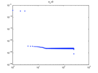
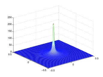
Figure 1: Distribution of singular values of ${\bf A}_{0}$ with $M=N=256$ and the magnitude of $\mathcal{I}_{\rm MU}$ on plane $z=0.0$.

We test the influence of the noisy measurements by adding a Gaussian noisy matrix with mean zero and variance $\sigma_{\rm n}^{2}/M$ to unperturbed response matrix ${\bf A}_{0}$. In our tests, the Gaussian noise is generated by MATLAB function randn. The imaging results shown in Figure 2 indicate that the imaging results become sharper as the noise level is smaller. Then we show the validity of (5.24). Noticing that $M=N$ makes $\gamma=1$ in our setting. By the analysis in Section 5, for given FAR $\delta$, POD depends on the ratio ${\sigma^{{\bf A}_{0}}_{1}}/{\sigma_{\rm n}}$. Here we only consider the critical regime in which $\sigma^{\bf A_{0}}_{1}$ is of the same order of $\sigma_{\rm n}$ (specially $\sigma^{\bf A_{0}}_{1}>\sigma_{\rm n}$). Fixing FAR $\delta$, for each ratio ${\sigma^{\bf A_{0}}_{1}}/{\sigma_{\rm n}}$, we generate 1000 Gaussian noisy matrices with mean zero and variance $\sigma_{\rm n}^{2}/M$ and add them to $\bf A_{0}$ to get according noisy response matrices $\bf A$. We compute $R$ with the help of SVD for each $\bf A$ and count the times for $R>r_{\delta}$ to get the numerical POD. Figure 3 shows the comparisons between numerical POD and (5.24) for each $\delta$. We can conclude that the numerical results are in good agreement with (5.24).

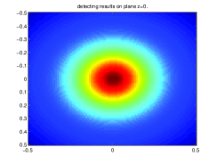
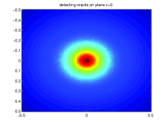
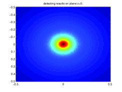
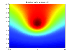
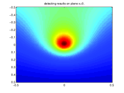
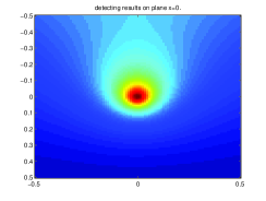
Figure 2: Detecting results on cross sectional plane $z=0$(top) and $x=0$(bottom) for different noise level $\sigma_{\rm n}$. $\sigma^{\bf A_{0}}_{1}/\sigma_{\rm n}=10,20,30$ from left to right.

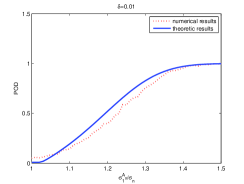
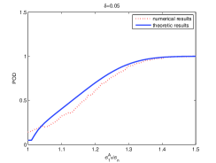
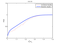
Figure 3: POD with respect to $\sigma^{\bf A_{0}}_{1}/\sigma_{\rm n}$ for different $\delta$, $\delta=0.01,0.05,0.10$ from left to right.

7 Concluding Remarks

In this paper we have provided an asymptotic expansion for the perturbations of the magnetic field due to the presence of an arbitrary shaped small conductive inclusion with smooth boundary and constant permeability and conductivity parameters. This was done under the assumption that the characteristic size of the inclusion is of the same order of magnitude as the skin depth. Our analysis can be extended to the case of variable permeability and conductivity distributions. We expect, however, that dealing with nonsmooth inclusions is challenging.

Our asymptotic formula was in turn used to construct a method for localizing conductive targets. We also presented numerical simulations for illustration. Thinking ahead, it appears that it would be very interesting to apply the findings from this paper to real-time target identification in eddy current imaging using the so called dictionary matching method [1, 2]. We are also interested in investigating target tracking from induction data at multiple frequencies. In the presence of noise, another problem of interest is to study how to estimate resolution for the localization of targets. This will be the subject of a forthcoming publication.

References

• [1] H. Ammari, T. Boulier, J. Garnier, W. Jing, H. Kang, and H. Wang, Target identification using dictionary matching of generalized polarization tensors, arXiv:1204.3035.
• [2] H. Ammari, T. Boulier, J. Garnier, and H. Wang, Shape recognition and classification in electro-sensing, arXiv:1302.6384.
• [3] H. Ammari, A. Buffa, and J.C. Nédélec, A justification of eddy currents model for the Maxwell equations, SIAM J. Appl. Math., 60 (2000), 1805–1823.
• [4] H. Ammari, J. Garnier, H. Kang, W.-K. Park, and K. Sølna, Imaging schemes for perfectly conducting cracks, SIAM J. Appl. Math., 71 (2011), 68–91.
• [5] H. Ammari, J. Garnier, and K. Sølna, A statistical approach to target detection and localization in the presence of noise, Waves Random Complex Media, 22 (2012), 40–65.
• [6] H. Ammari, E. Iakovleva, D. Lesselier, and G. Perrusson, A MUSIC-type electromagnetic imaging of a collection of small three-dimensional inclusions, SIAM J. Sci. Comput., 29 (2007), 674–709.
• [7] H. Ammari and H. Kang, Reconstruction of small inhomogeneities from boundary measurements, vol. 1846, Lecture Notes in Mathematics, Springer-Verlag, Berlin, 2004.
• [8] H. Ammari and H. Kang, Polarization and Moment Tensors: with Applications to Inverse Problems and Effective Medium Theory, Applied Mathematical Sciences, Vol. 162, Springer-Verlag, New York, 2007.
• [9] H. Ammari and A. Khelifi, Electromagnetic scattering by small dielectric inhomogeneities, J. Math. Pures Appl., 82 (2003), 749–842.
• [10] H. Ammari, M. Vogelius, and D. Volkov, Asymptotic formulas for perturbations in the electromagnetic fields due to the presence of inhomogeneities of small diameter II. The full Maxwell equations, J. Math. Pures Appl., 80 (2001), 769–814.
• [11] H. Ammari and D. Volkov, The leading-order term in the asymptotic expansion of the scattering amplitude of a collection of Finite Number of dielectric inhomogeneities of small diameter, Int. J. Mult. Comput. Eng., 3 (2005), 149–160.
• [12] B. A. Auld and J. C. Moulder, Review of advances in quantitative eddy current nondestructive evaluation, J. Nondest. Eval., 18 (1999), 3–36.
• [13] J. Baik, G. Ben Arous, and S. Péché, Phase transition of the largest eigenvalue for nonnull complex sample covariance matrices, Ann. Probab., 33 (2005), 1643–1697.
• [14] G. Benaych and R. R. Nadakuditi, The singular values and vectors of low rank perturbations of large rectangular random matrices, J. Multivariate Analysis, 111 (2012), 120–135.
• [15] M. Capitaine, C. Donati-Martin, and D. Féral, Central limit theorems for eigenvalues of deformations of Wigner matrices, Ann. Inst. H. Poincar Probab. Statist., 48 (2012), 107–133.
• [16] D. J. Cedio-Fengya, S. Moskow, and M. S. Vogelius, Identification of conductivity imperfections of small diameter by boundary measurements: Continuous dependence and computational reconstruction, Inverse Problems, 14 (1998), 553–595.
• [17] J. Garnier and K. Sølna, Applications of random matrix theory for sensor array imaging with measurement noise, submitted to special MSRI volume.
• [18] R. Hiptmair, Symmetric coupling for eddy current problems, SIAM J. Numer. Anal. 40 (2002), 41-65.
• [19] I. M. Johnstone, On the distrbution of the largest eigenvalue in principal components analysis, Ann. Statist., 29 (2001), 295–327.
• [20] V. A. Marcenko and L. A. Pastur, Distributions of eigenvalues of some sets of random matrices, Math. USSR-Sb., 1 (1967), 507–536.
• [21] J. C. Nédélec, Acoustic and Electromagnetic Equations: Integral Representations for Harmonic Problems, Springer, 2001.
• [22] S. J. Norton and I. J. Won, Identification of buried unexploded ordnance from broadband electromagnetic induction data, IEEE Trans. Geoscience Remote Sensing, 39 (2001), 2253–2261.
• [23] J. Rosell, R. Casanas, and H. Scharfetter, Sensitivity maps and system requirements for magnetic induction tomography using a planar gradiometer, Physiol. Meas., 22 (2001), 212–130.
• [24] J. Seberry, B. J. Wysocki, and T. A. Wysocki, On some applications of Hadamard matrices, Metrika, 62 (2005), 221–239.
• [25] A. Valli, Solving an electrostatics-like problem with a current dipole source by means of the duality method, Appl. Math. Lett., 25 (2012), 1410–1414.