Inflation and Birth of Cosmological Perturbations

Abstract

We review recent developments in the theory of inflation and cosmological perturbations produced from inflation. After a brief introduction of the standard, single-field slow-roll inflation, and the curvature and tensor perturbations produced from it, we discuss possible sources of nonlinear, non-Gaussian perturbations in other models of inflation. Then we describe the so-called $\delta N$ formalism, which is a powerful tool for evaluating nonlinear curvature perturbations on super Hubble scales.

I Introduction

One of the most successful applications of the theory of general relativity is cosmology. Over the past half century the big-bang theory of the universe, that the universe was born in an extremely hot and dense state, expanded explosively and cooled down to the present state, was observationally tested from various aspects and it is now firmly established. According to the big-bang theory, our universe is about 14 Giga years old, and the universe was radiation-dominated in the beginning. It became matter-dominated when the universe was about 100,000 years old, which happens to be about the same time when the photons decoupled from baryons, and started to travel freely until today, which are observed as the cosmic microwave background (CMB) radiation. The epoch when the CMB photons were scattered last before they reach us forms a 3-dimensional hypersurface, and it is called the last scattering surface (LSS).

Despite its tremendous success, there are still a couple of very basic problems that the big-bang theory cannot explain. One of them is the horizon problem or perhaps better to be called the causality problem, and the other the flatness problem or the entropy problem.

I.1 Horizon problem

Let us first consider the horizon problem. The big-bang theory assumes an homogeneous and isotropic universe on large scales. So the metric is assumed to be in the form,

$$ds^{2}=-dt^{2}+a^{2}(t)d\sigma_{(3)}^{2}\,,$$ (1)

where $d\sigma_{(3)}^{2}$ is the 3-metric of a constant curvature space with $K$ being the curvature, ${}^{(3)}R^{ij}{}_{km}=K(\delta^{i}_{k}\delta^{j}_{m}-\delta^{i}_{m}\delta^{j}_{k})$. A coordinate system that spans $d\sigma_{(3)}^{2}$ is said to be comoving because an observer staying at a fixed point on the 3-space is comoving with the expansion of the universe. In this spacetime, the time-time component of the Einstein equations, the Friedmann equation, is

$$H^{2}=\frac{\rho}{3M_{pl}^{2}}-\frac{K}{a^{2}}\,;\quad H\equiv\frac{\dot{a}}{a}\,,$$ (2)

where $M_{pl}^{2}=(8\pi G)^{-1}$ in the units $\hbar=c=1$, and the trace of the space-space components of the Einstein equations gives

$$\frac{\ddot{a}}{a}=-\frac{\rho+3P}{3M_{pl}^{2}}\,,$$ (3)

where $\rho$ is the energy density and $P$ is the pressure of the universe. This latter equation shows that the expansion of the universe is always decelerating as long as $\rho+3P>0$, which holds for both radiation $P=\rho/3$ and matter $P=0$. For simplicity, if we assume a simple equation of state $P/\rho=w=$constant and $K=0$ (which should be a good approximation in the early universe when $w=1/3$ since $\rho\propto a^{-3(1+w)}=a^{-4}$), one finds

$$a\propto t^{n}\,;\quad n=\frac{2}{3(1+w)}<1\quad\mbox{for}~{}w>-\frac{1}{3}\,.$$ (4)

This result may be regarded as a consequence of the attractive nature of the gravitational force.

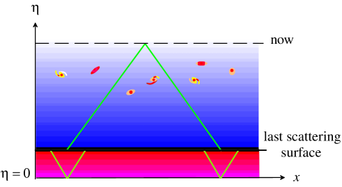
Figure 1: Horizon problem. The conformal time of the last scattering surface $\eta_{LSS}$ from $\eta=0$ is about 1/30 of that of today $\eta_{0}$.

Now we introduce the conformal time $d\eta=dt/a(t)$, and rewrite the metric as

$$ds^{2}=a^{2}(\eta)d\hat{s}^{2}\,;\quad d\hat{s}^{2}=-d\eta^{2}+d\sigma_{(3)}^{2}\,.$$ (5)

Since the conformal transformation of the metric does not change the causal structure, the static metric $d\hat{s}^{2}$ perfectly describes the causal structure of the universe. If the range of $\eta$ were infinite to the past, there would be no horizon problem. The problem is that the conformal time is finite in the past if $w>-1/3$ or $\rho+3P>0$, because

$$\eta=\int_{0}^{t}\frac{dt^{\prime}}{a(t^{\prime})}\propto\int_{0}^{t}\frac{dt^{\prime}}{t^{\prime}{}^{n}}\,;\quad n=\frac{2}{3(1+w)}\,.$$ (6)

This implies that the size of lightcone emanating from a point at the beginning of the universe when $\eta=0$ will cover only a finite fraction of spacetime. Since the comoving distance traveled by light is equal to the corresponding conformal time interval, the comoving radius of the causally connected region on the LSS is equal to its conformal time $\eta_{LSS}$. From the fact that the LSS is located at redshift $z\sim 10^{3}$ and the universe is approximately matter-dominated since then, one finds that this region will cover only a tiny fraction (about $10^{-3}$ sr) of the sky. This is the horizon problem (see Fig. 1).

The solution is clear: The horizon problem disappears if the conformal time is either infinite in the past or the beginning of the universe $\eta=0$ is extended sufficiently back in time to cover the whole visible universe. Since the comoving radius of the visible universe on the LSS is $\eta_{0}-\eta_{LSS}$ where $\eta_{0}$ is the conformal time today, the problem is solved if $\eta_{LSS}>\eta_{0}-\eta_{LSS}$. In Einstein gravity, this means that the equation of state must be $w<-1/3$ or the expansion of the universe must be accelerating ($\ddot{a}>0$) for a sufficient lapse of time in the very early universe.

Here we should note that solving the horizon problem does not mean explaining the homogeneity and isotropy of the universe. As clear from the above argument, we had to assume the homogeneity and isotropy of the universe to pose the horizon problem. This point is very often misunderstood in the literature.

I.2 Flatness problem

Again we assume a spatially homogeneous and isotropic universe, Eq. (1). The Friedmann equation (2) tells us that the curvature term $K/a^{2}$ is completely negligible in the early universe when $\rho\propto a^{-4}$. Conversely, if the curvature term was of the same order of magnitude as the density at an epoch in the early universe, the universe must have either collapsed (if $K>0$) or become completely empty (if $K<0$) by now.

Alternatively, since the energy density is dominated by radiation in the early universe and so is the entropy of the universe, the problem may be rephrased as the existence of huge entropy within the curvature radius of the universe,

$$S=T^{3}\left(\frac{a}{\sqrt{|K|}}\right)^{3}\approx T_{0}^{3}\left(\frac{a_{0}}{\sqrt{|K|}}\right)^{3}>T_{0}^{3}H_{0}^{3}\approx 10^{87}\,,$$ (7)

where $T_{0}\approx 2.7$ K is the CMB temperature today Mather:1993ij and $H_{0}\approx 72$ km/s/Mpc is the Hubble constant Freedman:2010xv . Hence the flatness problem may be called the entropy problem.

It is then apparent that the solution to the flatness problem needs huge entropy production at a sufficiently early stage of the universe.

I.3 Inflation as a solution to horizon and flatness problems

A simple and perhaps the best solution to the horizon and flatness problems is given by the inflationary universe Sato:1980yn ; Guth:1980zm . Let us assume that the universe was dominated by a spatially homogeneous scalar field. For a minimally coupled canonical scalar field $\phi$, we have

$$\rho=\frac{1}{2}\dot{\phi}^{2}+V(\phi)\,,\quad P=\frac{1}{2}\dot{\phi}^{2}-V(\phi)\,,$$ (8)

so $\rho+3P=2\bigl{(}\dot{\phi}^{2}-V(\phi)\bigr{)}$. Hence if $\dot{\phi}^{2}<V(\phi)$, we may have accelerated expansion. In particular, if the energy density is dominated by the potential energy, $\dot{\phi}^{2}\ll V(\phi)$, the motion of the scalar field can be ignored within a few expansion times $\sim H^{-1}$, and the universe expands almost exponentially,

$$H^{2}\approx\frac{\rho}{3M_{pl}^{2}}\approx\mbox{constant}.$$ (9)

The curvature term $K/a^{2}$ becomes completely negligible.

Thus if the universe is dominated by the potential energy, or the vacuum energy, and the potential energy is converted to radiation after a sufficient lapse of time of such a stage, a huge entropy is produced and the horizon and flatness problems are solved simultaneously.

II Slow-roll inflation and vacuum fluctuations

There have been a number of proposals for inflationary models. Among others, a simplest class of models, and which explains the observational data almost perfectly, is the slow-roll infation Linde:1981mu ; Albrecht:1982wi ; Linde:1983gd . The field equation for $\phi$ and the Friedmann equation are

$$\ddot{\phi}+3H\dot{\phi}+V^{\prime}(\phi)=0\,,\quad H^{2}=\frac{1}{3M_{pl}^{2}}\left[\frac{1}{2}\dot{\phi}^{2}+V(\phi)\right]\,,$$ (10)

where we have justifiably neglected the curvature term.

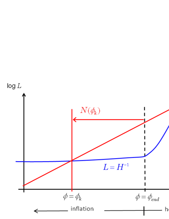
Figure 2: The Hubble radius$L=H^{-1}$ and the length scale $L=a/k$ of a comoving wavenumber $k$ in the inflationary cosmology, and the definition of the number of $e$-folds $N(\phi)$.

The standard slow-roll condition consists of two assumptions. One is that $\ddot{\phi}$ is negligible compared to $3H\dot{\phi}$ in the field equation, that is, the equation of motion is friction-dominated. The other is that the kinetic term $\dot{\phi}^{2}/2$ is negligible compared to the potential term $V$ in the energy density. Under this condition we have

$$\dot{\phi}=-\frac{V^{\prime}(\phi)}{3H}\,;\quad H^{2}=\frac{V}{3M_{pl}^{2}}\,.$$ (11)

Then the potential energy dominance implies

$$\epsilon\equiv-\frac{\dot{H}}{H^{2}}=\frac{\dfrac{3}{2}\dot{\phi}^{2}}{\dfrac{1}{2}\dot{\phi}^{2}+V}\approx\frac{3\dot{\phi}^{2}}{2V}\approx\frac{M_{pl}^{2}}{2}\frac{V^{\prime}{}^{2}}{V^{2}}\equiv\epsilon_{V}\ll 1\,,$$ (12)

that is, the universe is expanding almost exponentially, and the friction-dominated equation of motion $|\ddot{\phi}/(3H\dot{\phi})|\ll 1$ implies

$$\frac{V^{\prime\prime}}{3H^{2}}\approx M_{pl}^{2}\frac{V^{\prime\prime}}{V}\equiv\eta_{V}\ll 1\,.$$ (13)

The single-field slow-roll inflation satisfies these conditions.

The important property of slow-roll inflation is that Eq. (11) is completely integrable since $H$ is a function of $\phi$. In particular, there is one-to-one correspondence between $\phi$ and $t$. So instead of the cosmic time $t$ we may measure the time in terms of the value of the scalar field.

Here we introduce a quantity which plays a very important role in the dynamics of slow-roll inflation, namely the number of $e$-folds counted backward in time, say from the end of inflation to an epoch during inflation,

$$\frac{a(t_{end})}{a(t)}=\exp[N(t\to t_{end})]~{}\to~{}N=N(\phi)=\int_{t(\phi)}^{t_{end}}Hdt\,.$$ (14)

Its important property is that by definition it does not depend on how and when the inflation began. As shown in Fig. 2, $N$ is uniquely determined in terms of the value of the scalar field (up to a constant which depends on the choice of an epoch from which $N$ is computed), and one can associate $N$ with the time at which a given comoving wavenumber $k$ crossed the Hubble radius, $k=aH$, at which the value of the scalar field was $\phi_{k}$; $N=N(\phi_{k})$. As we shall see below, this turns out to be an essential quantity for the evaluation of the curvature perturbation from inflation.

II.1 Curvature perturbation

Let us now consider the curvature perturbation produced from inflation. It arises from the quantum vacuum fluctuations of the inflaton field $\phi$. Since a rigorous derivation would take too much space, here we give an intuitive, rather hand-waving derivation. We caution that it could well lead to an incorrect result if used blindly.

The vacuum fluctuations of the inflaton field with a comoving wave number $k$ is given simply by its positive frequency function, $\varphi_{k}$. Because of the condition $V^{\prime\prime}/H^{2}\ll 1$, on scales $k/a\gg H$, the inflaton field fluctuation behaves like a minimally coupled massless scalar. Hence we have

$$\left|\langle\delta\phi|\vec{k}\rangle\right|^{2}=|\varphi_{k}|^{2}\,,\quad\varphi_{k}\sim\frac{1}{a^{3/2}\sqrt{2\omega_{k}}}e^{-i\omega_{k}t}\,;\quad\omega_{k}=\frac{k}{a}\gg H\,.$$ (15)

As the universe expands the physical wavenumber decreases exponentially and becomes smaller than the Hubble parameter, $k/a<H$, or the physical wavelength exceed the Hubble radius. Then the oscillations of $\varphi_{k}$ are frozen. This could be regarded as “classicalization’ of the quantum fluctuations. Not that this is merely an interpretation. In a more rigorous sense, freezing of the mode function is a process toward infinite squeezing of the vacuum state.

Setting $a=k/H$ in Eq. (15) gives

$$\varphi_{k}\sim\frac{H}{\sqrt{2k^{3}}}\,;\quad\frac{k}{a}\ll H\,.$$ (16)

Therefore the mean square amplitude in unit logarithmic interval of $k$ is

$$\langle\delta\phi^{2}\rangle_{k}\equiv\frac{4\pi k^{3}}{(2\pi)^{3}}|\varphi_{k}|^{2}\approx\left(\frac{H}{2\pi}\right)_{k/a=H}^{2}\,.$$ (17)

Inclusion of the non-trivial evolution of the background spacetime and the coupling of the scalar field fluctuation with the metric fluctuation do not change the above estimate if we interpret $\delta\phi$ in the above as those evaluated on the flat slicing, that is, on hypersurfaces on which the spatial scalar curvature remains unperturbed.

It is known that the curvature perturbation on the comoving hypersurface ${\cal R}_{c}$ is conserved if the perturbation is adiabatic Kodama:1985bj . The comoving hypersurface is defined as a surface of uniform $\phi$. Then the gauge transformation from the flat slicing to the comoving slicing gives the relation between ${\cal R}_{c}$ and $\delta\phi$,

$${\cal R}_{c}=-\frac{H}{\dot{\phi}}\delta\phi\,.$$ (18)

Since this is conserved for $k/a<H$, the spectrum of the comoving curvature perturbation in unit logarithmic interval of $k$ is given by

$${\cal P}_{\cal R}(k)\equiv\frac{4\pi k^{3}}{(2\pi)^{3}}|{\cal R}_{k}|^{2}\approx\left(\frac{H^{2}}{2\pi\dot{\phi}}\right)_{k/a=H}^{2}\,.$$ (19)

A rigorous, first-principle derivation of the above result was first done in Mukhanov:1985rz ; Sasaki:1986hm .

The important relation of the above result with the number of $e$-folds was first pointed out in Starobinsky:1986fxa : If we rewrite Eq. (14) as

$$N=\int_{t}^{t_{end}}Hdt=\int_{\phi}^{\phi_{end}}\frac{H}{\dot{\phi}}d\phi\,,$$ (20)

we find

$$\delta N(\phi_{k})=\left[\frac{\partial N}{\partial\phi}\delta\phi\right]_{k/a=H}=\left[-\frac{H}{\dot{\phi}}\delta\phi\right]_{k/a=H}={\cal R}_{c}\,,$$ (21)

provided that we identify $\delta\phi$ with the scalar field fluctuation evaluated on the flat hypersurface. This is called the $\delta N$ formula.

The $\delta N$ formula implies that we only need the knowledge of the background evolution to obtain the power spectrum of the comoving curvature perturbation, once we know the amplitude of the quantum fluctuations of the scalar field at the horizon crossing (i.e. when $k/a=H$). It is quite generally given by $H/(2\pi)$ in slow-roll inflation. With careful geometrical considerations, the $\delta N$ formula can be extended to general multi-field inflation Sasaki:1995aw ,

$${\cal P}_{\cal R}(k)=\left(\frac{H}{2\pi}\right)^{2}||\nabla N||^{2};\quad||\nabla N||^{2}\equiv G^{ab}(\phi)\frac{\partial N}{\partial\phi^{a}}\frac{\partial N}{\partial\phi^{b}}\,,$$ (22)

where $G^{ab}$ is the field space metric and it is assumed that the vacuum expectation values are given by

$$\langle\delta\phi^{a}\delta\phi^{b}\rangle=G^{ab}\left(\frac{H}{2\pi}\right)^{2}\,.$$ (23)

The nonlinear generalization of the $\delta N$ formalism will be discussed in Sec. IV.

II.2 Tensor perturbation

There are not only vacuum fluctuations of the inflaton field but also those of the transverse-traceless part of the metric, $\partial^{i}h_{ij}^{TT}=\delta^{ij}h_{ij}^{TT}=0$, that is, the tensor perturbation or gravitational wave degrees of freedom. If we construct the second-order action for $h_{ij}^{TT}$, we find

$$S\sim\frac{M_{pl}^{2}}{8}\int d^{4}x\sqrt{-g}(\dot{h}_{ij}^{TT})^{2}+\cdots.$$ (24)

To quantize $h_{ij}^{TT}$ it is convenient to normalize the kinetic term to the canonical form. This gives

$$S\sim\frac{1}{2}\int d^{4}x\sqrt{-g}(\dot{\phi}_{ij})^{2}+\cdots\,;\quad\phi_{ij}\equiv\frac{M_{pl}}{2}h_{ij}^{TT}.$$ (25)

If one writes down the field equation for $\phi_{ij}$, one finds its mode function $\phi_{k}$ obeys exactly the same equation as the one for a minimally coupled massless scalar field,

$$\ddot{\phi}_{k}+3H\dot{\phi}_{k}+\frac{k^{2}}{a^{2}}\phi_{k}=0\,.$$ (26)

Since there are two independent degrees of freedom in $\phi_{ij}$, the power spectrum of the tensor perturbation $h_{ij}^{TT}$ is obtained as

$${\cal P}_{T}(k)=\frac{4}{M_{pl}}\times 2\times\frac{4\pi k^{3}}{(2\pi)^{3}}|\phi_{k}|^{2}=\frac{8H^{2}}{(2\pi)^{2}M_{pl}^{2}}\,.$$ (27)

Taking the ratio of the tensor spectrum to the curvature perturbation spectrum, we find Sasaki:1995aw

$$r\equiv\frac{{\cal P}_{T}}{{\cal P}_{\cal R}}\leq 8|n_{T}|=-2\frac{\dot{H}}{H^{2}}\,,$$ (28)

where $n_{T}$ is the tensor spectral index, $n_{T}=d\ln{\cal P}_{T}(k)/d\ln k$, and the equality holds for the case of single-field slow-roll inflation. This is a consistency relation in general slow-roll inflation. As a proto-type example, if we consider chaotic inflation Linde:1983gd , we expect to have $r\sim 0.1$.

The important point to be kept in mind is that the existence of the vacuum fluctuations of the tensor part of the metic is a proof of the existence of quantum gravity. These fluctuations exist in any theory of gravity that respects general covariance, apart from possible inessential modifications of the spectrum. Thus a clear detection of the tensor spectrum will be a confirmation of not only the inflationary universe but also quantum gravity.

III Origin of non-Gaussianity

The standard, single-field slow-roll inflation predicts that the curvature perturbation is a Gaussian random field and it has an almost scale-invariant spectrum. This seems to fit the current observational data quite well Komatsu:2010fb , it is quite possible that the actual model turns out to be non-standard. Maybe it is multi-field, maybe non-slow-roll and/or non-canonical. In such a case, the curvature perturbation may become non-Gaussian. Search for possible non-Gaussian signatures in the primordial curvature perturbation has become one of the important directions in observation in recent years Komatsu:2009kd .

Here we consider possible origins of non-Gaussianity in the curvature perturbation. Essentially one can classify the origins into three categories: (1) Self-interactions of the inflaton field and/or non-trivial vacua, (2) multi-field dynamics, and (3) nonlinearity in gravity.

The non-Gaussianities of the first category are generated on subhorizon scales during inflation, hence they are of quantum field theoretical origin. Those of the second category are usually generated on superhorizon scales either during or after inflation, and they are due to nonlinear coupling of the scalar field to gravity. Since they are generated on superhorizon scales, they are of classical origin. Finally those of the third category are due to nonlinear dynamics in general relativity. Hence they are generated after the scale of interest re-enters the Hubble horizon. Since the last category is not really primordial in nature, let us focus on the first two categories.

III.1 Non-Gaussianity from self-interaction/non-trivial vacuum

It is known that conventional self-interactions by the potential are ineffective Maldacena:2002vr . This can be seen by considering chaotic inflation, for example. In the simplest case of a quadratic potential, $V=m^{2}\phi^{2}/2$, the inflaton is actually a free field apart from the interaction through gravitation perturbations. But the gravitational interaction is Planck-suppressed, i.e., it is always suppressed by a factor $O(M_{pl}^{-2})$. In the case of a quartic potential, $V=\lambda\phi^{4}$, it is known that $\lambda$ should be extremely small $\lambda\sim 10^{-15}$ in order for it to be consistent with observation.

Thus some kind of unconventional self-interaction is necessary. A popular example is the case of a scalar field with a non-canonical kinetic term such as DBI inflation Alishahiha:2004eh . In this case the kinetic term takes the form,

$$K\sim f^{-1}(\phi)\sqrt{1-f(\phi)\dot{\phi}^{2}}\equiv f^{-1}\gamma^{-1}\,.$$ (29)

If we expand this perturbatively,

$$K=K_{0}+\delta_{1}K+\delta_{2}K+\delta_{3}K+\cdots,$$ (30)

we will find

$$\delta_{2}K\propto\gamma^{3}\,,\quad\delta_{3}K\propto\gamma^{3+2}\,,$$ (31)

since $\delta\gamma=\gamma^{3}\delta X$ where $X\equiv f\dot{\phi}^{2}/2$. If we regard the third order part as the interaction, the above implies that the scalar field fluctuation will be expressed qualitatively as

$$\delta\phi\sim\delta\phi_{0}+\gamma^{2}\delta\phi_{0}^{2}+\cdots,$$ (32)

where $\delta\phi_{0}$ is the free, Gaussian fluctuation. Thus the non-Gaussianity in $\delta\phi$ may become large if $\gamma$, which mimics the Lorentz factor, is large Mizuno:2009cv .

A non-trivial vacuum state is another source of non-Gaussianity. If the universe were a pure de Sitter spacetime, gravitational interaction would be totally negligible in vacuum, except for the effect due to graviton (tensor mode) loops. This may be regarded as due to the maximally symmetric nature of the de Sitter space, $SO(4,1)$, which has the same number of degrees of symmetry as the Poincare (Minkowski) symmetry. In slow-roll inflation, the de Sitter symmetry is slightly broken. Nevertheless the effect induced by this symmetry breaking is small because it is suppressed by the slow-roll parameter $\epsilon=-\dot{H}/H^{2}$.

However, if the vacuum state does not respect the de Sitter symmetry, there can be a large non-Gaussianity. Such a deviation from the quasi-de Sitter vacuum, usually called the Bunch-Davies vacuum, may occur in various situations, studied e.g. in Chen:2008wn ; Flauger:2009ab .

III.2 Non-Gaussianity from multi-field dynamics

Non-Gaussianity may appear if the energy momentum tensor depends nonlinearly on the scalar field even if the fluctuation of the scalar filed itself is Gaussian. This effect is generally important when the fluctuations are on superhorizon scales, i.e., the characteristic wavelength is larger than the Hubble radius. It is small in single-field slow-roll models because the linear approximation is valid to high accuracy Salopek:1990jq , generically suppressed by the slow-roll parameter $\eta_{V}$ defined in Eq. (13).

For multi-field models, however, the contribution to the energy momentum tensor from some of the fields can be highly nonlinear as depicted in Fig. 3.

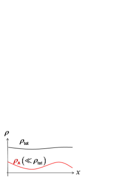
Figure 3: An illustration of the energy density configuration in the multi-field case. The density of the $A$-matter/field $\rho_{A}$ may vary nonlinearly without significantly affecting the total energy density.

The important property of non-Gaussianity in this case is that it is always of the spatially local type. Namely, to second order in nonlinearity, the curvature perturbation will take the form Komatsu:2001rj ,

$${\cal R}_{c}(x)={\cal R}_{c,0}(x)+\frac{3}{5}f_{NL}^{\rm local}\,{\cal R}_{c,0}^{2}(x)\,,$$ (33)

where ${\cal R}_{c,0}$ is the Gaussian random field and $f_{NL}^{\rm local}$ is a constant representing the amplitude of non-Gaussianity. The factor 3/5 in front of $f_{NL}^{\rm local}$ is due to a historical reason. The reason why it is of local type is simply causality: No information can propagate over a length scale greater than the Hubble horizon scale.

Observationally, this type of non-Gaussianity can be tested by using the so-called squeezed type templates where one of the wavenumbers, say $k_{1}$ in the bispectrum $B({\vec{k}}_{1},{\vec{k}}_{2},{\vec{k}}_{3})$ is much smaller than the other two, $k_{1}\ll k_{2}\approx k_{3}$ Komatsu:2009kd , and there are a few observational indications that $f_{NL}^{\rm local}$ is actually non-vanishing. For example, the WMAP 7 year data analysis gave a one-sigma bound $11<f_{NL}^{\rm local}<53$ ($68\%$ CL) Komatsu:2010fb .

IV $\bm{\delta N}$ formalism

As mentioned in Sec. II, the $\delta N$ formalism is a powerful tool to evaluate the comoving curvature perturbation on superhorizon scales. It then turned out that it can be easily extended to the evaluation of nonlinear, non-Gaussian curvature perturbations Lyth:2004gb ; Lyth:2005fi . Let us recapitulate its definition and properties:

• $\delta N$ is the perturbation in the number of $e$-folds counted backward in time from a fixed final time, say $t=t_{f}$, to some initial time $t=t_{i}$.

• The final time $t_{f}$ should be chosen such that the evolution of the universe has become unique by that time, i.e., the universe has reached the adiabatic limit. Then the hypersurface $t=t_{f}$ should be identified with a comoving (or uniform density) slice, and the initial hypersurface $t=t_{i}$ should be identified with a flat slice.

• $\delta N$ is equal to the conserved (nonlinear) comoving curvature perturbation on superhorizon scales at $t>t_{f}$.

• By definition, it is nonlocal in time. However, because of its purely geometrical definition, it is valid independent of which theory of gravity one considers, provided that the adiabatic limit is reached by $t=t_{f}$.

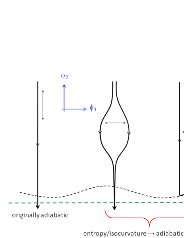
Figure 4: Three different types of $\delta N$. The field space $(\phi_{1},\phi_{2})$ in the figure represents the degrees of freedom in the initial condition of the universe. The adiabatic limit is defined to be the stage by which all the trajectories converge to a unique one.

There are various kinds of sources that generate $\delta N$. They may be classified into three types, as depicted in Fig. 4. The left one describes a perturbation along the evolutionary trajectory of the universe. This case is the same as that of single-field slow-roll inflation, in which the comoving curvature perturbation is conserved all the way until it re-enters the horizon. The middle one is the case when a small difference in the initial data develops into a substantial difference in $\delta N$. Typically this is realized when there is some instability orthogonal to the trajectory, like the case when the scalar field moves along a ridge. This type of sources of $\delta N$ usually induces a feature in the spectrum and/or bispectrum of the curvature perturbation. The right one represents the case when the perturbation orthogonal to the trajectory does not contribute to the curvature perturbation until or after the end of inflation, but $\delta N$ is generated due to a sudden transition that brings the universe into an adiabatic stage. Typical examples are curvaton models Lyth:2001nq ; Moroi:2001ct ; Sasaki:2006kq and multi-brid inflation models Sasaki:2008uc ; Naruko:2008sq .

Here, for the sake of completeness, let us present the precise definition of the nonlinear $\delta N$ formula. See Fig. 5. It is based on the leading order approximation in the spatial gradient expansion or the separate universe approach Lyth:2004gb , where spatial derivatives are assumed to be negligible in comparison with time derivatives. At leading order of the spatial gradient expansion, if we express the spatial volume element as $\sqrt{{}^{(3)}\gamma}=a^{3}(t)\exp[3{\cal R}(t,x)]$ where $a(t)$ is the scale factor of a fiducial homogeneous and isotropic universe, we easily find that the perturbation in the number of $e$-folds along a comoving trajectory between two hypersurfaces $t=t_{1}$ and $t=t_{2}$ is given by

$$\delta N(t_{2},t_{1};x^{i})={\cal R}(t_{2},x^{i})-{\cal R}(t_{1},x^{i})\,,$$ (34)

where $x^{i}$ are the comoving coordinates. Here we note that this is purely a geometrical relation. It has nothing to do with any equations of motion.

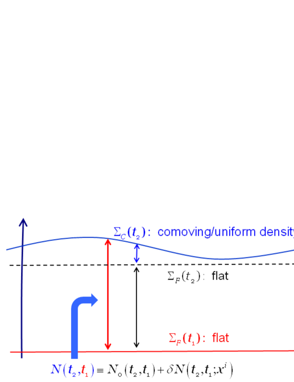
Figure 5: Definition of nonlinear $\delta N$. It is defined as the perturbation in the number of $e$-folds from an initial flat slice to a final comoving slice.

First we fix the final hypersurface $t=t_{2}$. It should be taken at the stage when the evolution of the universe has become unique. That is, there exists no isocurvature perturbation any longer that could develop into an adiabatic perturbation at later epochs. Thus the comoving curvature perturbation is conserved at $t>t_{2}$. In the context of the concordance $\Lambda$CDM model of the universe, this corresponds to the final radiation-dominated stage of the universe.

Next we choose the initial slice $t=t_{1}$. It should be chosen to be flat. Here ‘flat’ means that the perturbation in the spatial volume element vanishes. Namely, the flat slice is defined as a hypersurface on which ${\cal R}=0$. We note that despite its name, the scalar curvature vanishes only in the linear theory limit: It is non-vanishing in general in the nonlinear case.

Applying the above choice of the initial and final hypersurfaces to Eq. (34), it is trivial to see that we have

$$\delta N(t_{2},t_{1};x^{i})={\cal R}_{c}(t_{2},x^{i})\,.$$ (35)

Now by assumption ${\cal R}_{c}$ is conserved at $t>t_{2}$. So it is the quantity we want to evaluate. This completes the derivation of the nonlinear $\delta N$ formula.

As mentioned above, since Eq. (34) is a pure geometrical relation, so is the nonlinear $\delta N$ formula (35). This is the reason why it can be applied to any theory of gravity as long as it is a geometrical (i.e. general covariant) theory.

Of course, the above definition tells us nothing about how to evaluate it in practice. In this respect, we have a very fortunate situation in the case of inflationary cosmology. It is the fact that the evaluation of the quantum fluctuations of the inflaton field, whether it is single- or multi-component, can be most easily done in a gauge in which the time slicing is chosen to be flat Sasaki:1995aw . Thus we can choose the initial slice to be an epoch when the scale of our interest has just exited the horizon during inflation. Let the fluctuations of a multi-component scalar field on the flat slice at $t=t_{1}$ to be $\delta\phi^{a}$. Then assuming that the values of the scalar field determine the evolution of the universe completely, which is the case for slow-roll inflation, the nonlinear $\delta N$ can be simply evaluated as

$$\delta N=N(\phi^{a}+\delta\phi^{a})-N(\phi^{a})\,,$$ (36)

where $N(\phi^{a})$ is the $e$-folding number of the fiducial background. In particular, to second order in $\delta\phi^{a}$, we obtain

$${\cal R}_{c}=\delta N=\frac{\partial N}{\partial\phi^{a}}\delta\phi^{a}+\frac{1}{2}\frac{\partial^{2}N}{\partial\phi^{a}\partial\phi^{b}}\delta\phi^{a}\delta\phi^{b}+\cdots\,,$$ (37)

Comparing this with Eq. (33), we see that the curvature perturbation takes a bit more complicated form that the simplest form. Nevertheless if we consider the bispectrum, i.e., the Fourier component of the three-point function $\langle{\cal R}_{c}(x_{1}){\cal R}_{c}(x_{2}){\cal R}_{c}(x_{3})\rangle$, we find there is a quantity that exactly corresponds to $f_{NL}^{\rm local}$ defined in Eq. (33). Namely Lyth:2005fi ,

$$\frac{3}{5}f_{NL}^{\rm local}=\frac{G^{ab}G^{cd}N_{a}N_{bc}N_{d}}{2\left(||\nabla N||^{2}\right)^{2}}\,;\quad N_{a}\equiv\frac{\partial N}{\partial\phi^{a}}\,,\ N_{ab}\equiv\frac{\partial^{2}N}{\partial\phi^{a}\partial\phi^{b}}\,.$$ (38)

Before concluding this section, we mention the fact that the $\delta N$ formalism does not require the scalar field fluctuations to be Gaussian. In fact, except for the last equation in the above, Eq. (38) which assumes the Gaussianity of $\delta\phi^{a}$, the general $\delta N$ formula (36) or its second order version (37) can be used for non-Gaussian $\delta\phi^{a}$ Byrnes:2007tm . Such a case may happen, for example, in multi-field DBI inflation.

V Summary

It has been about 30 years since the inflationary universe was first proposed, and there is increasing observational evidence that inflation did take place in the very early universe. Among others, the measured CMB temperature anisotropy is fully consistent with the predictions of inflation that the primordial curvature perturbation spectrum is almost scale-invariant and it is statistically Gaussian.

Inflation also predicts a scale-invariant tensor spectrum, and if the energy scale of inflation is high enough as in the case of chaotic inflation, the tensor-scalar ratio $r$ can be as large as 0.1. If this is the case, the tensor perturbation will be detected in the near future, and it will confirm not only the inflationary universe but also quantum gravity.

Even if the tensor perturbation will not be detected, there may be other interesting signatures of inflation. Non-Gaussianity from inflation is attracting attention as one of those signatures that can distinguish or constrain models of inflation significantly.

We discussed that the origins of primordial non-Gaussianities may be classified into three categories, according to different length scales on which different mechanisms are effective:

• Quantum theoretical origin on subhorizon scales during inflation.

• Classical nonlinear scalar field dynamics on superhorizon scales during or after inflation.

• Nonlinear gravitational dynamics after the horizon re-entry.

In particular we argued that non-Gaussianities in the second case are always of spatially local type. We then mentioned that there are three different kinds of situations in which such local non-Gaussianities can be generated, and described in some detail a very efficient method to compute them, namely, the $\delta N$ formalism.

Apparently identifying properties of primordial non-Gaussianities in the observational data is extremely important for understanding the physics of the early universe. Here we mentioned only the bispectrum or the 3-point function. But if it is detected, higher order $n$-point functions may become important as a model discriminator. Other types of non-Gaussianity discriminators may also become necessary.

What is important is that we are now beginning to test observationally the physics of the very early universe, the physics at an energy scale closer to the Planck scale, at a scale that can never be attained in high energy accelerator experiments.

Cosmology has become not only a precision science, but now it constitutes a truly indispensable part of fundamental physics. General relativity is the backbone of cosmology. I wonder what Einstein would say if he were here in this very exciting era – 100 years after he visited Prague.

References

References

- (1) J. C. Mather et al., Astrophys. J. 420, 439 (1994).
- (2) W. L. Freedman and B. F. Madore, Ann. Rev. Astron. Astrophys. 48, 673 (2010) [arXiv:1004.1856 [astro-ph.CO]].
- (3) K. Sato, Mon. Not. Roy. Astron. Soc. 195, 467 (1981).
- (4) A. H. Guth, Phys. Rev. D 23, 347 (1981).
- (5) A. D. Linde, Phys. Lett. B 108, 389 (1982).
- (6) A. Albrecht and P. J. Steinhardt, Phys. Rev. Lett. 48, 1220 (1982).
- (7) A. D. Linde, Phys. Lett. B 129, 177 (1983).
- (8) H. Kodama and M. Sasaki, Prog. Theor. Phys. Suppl. 78, 1 (1984).
- (9) V. F. Mukhanov, JETP Lett. 41, 493 (1985).
- (10) M. Sasaki, Prog. Theor. Phys. 76, 1036 (1986).
- (11) A. A. Starobinsky, JETP Lett. 42, 152 (1985).
- (12) M. Sasaki and E. D. Stewart, Prog. Theor. Phys. 95, 71 (1996). [astro-ph/9507001].
- (13) E. Komatsu et al. [WMAP Collaboration], Astrophys. J. Suppl. 192, 18 (2011) [arXiv:1001.4538 [astro-ph.CO]].
-
(14)
E. Komatsu et al.,
arXiv:0902.4759 [astro-ph.CO].
See also articles in the focus section, (ed.) M. Sasaki and D. Wands, “Non-linear and non-Gaussian cosmological perturbations,” Class. Quant. Grav. 27, 120301 (2010). - (15) J. M. Maldacena, JHEP 0305, 013 (2003) [astro-ph/0210603].
- (16) M. Alishahiha, E. Silverstein and D. Tong, Phys. Rev. D 70, 123505 (2004) [hep-th/0404084].
- (17) S. Mizuno, F. Arroja, K. Koyama and T. Tanaka, Phys. Rev. D 80, 023530 (2009) [arXiv:0905.4557 [hep-th]].
- (18) X. Chen, R. Easther and E. A. Lim, JCAP 0804, 010 (2008) [arXiv:0801.3295 [astro-ph]].
- (19) R. Flauger, L. McAllister, E. Pajer, A. Westphal and G. Xu, JCAP 1006, 009 (2010) [arXiv:0907.2916 [hep-th]].
- (20) D. S. Salopek and J. R. Bond, Phys. Rev. D 42, 3936 (1990).
- (21) E. Komatsu and D. N. Spergel, Phys. Rev. D 63, 063002 (2001) [astro-ph/0005036].
- (22) D. H. Lyth, K. A. Malik and M. Sasaki, JCAP 0505, 004 (2005). [astro-ph/0411220].
- (23) D. H. Lyth and Y. Rodriguez, Phys. Rev. Lett. 95, 121302 (2005) [astro-ph/0504045].
- (24) D. H. Lyth and D. Wands, Phys. Lett. B 524, 5 (2002) [hep-ph/0110002].
- (25) T. Moroi and T. Takahashi, Phys. Lett. B 522, 215 (2001) [Erratum-ibid. B 539, 303 (2002)] [hep-ph/0110096].
- (26) M. Sasaki, J. Valiviita and D. Wands, Phys. Rev. D 74, 103003 (2006) [astro-ph/0607627].
- (27) M. Sasaki, Prog. Theor. Phys. 120, 159 (2008) [arXiv:0805.0974 [astro-ph]].
- (28) A. Naruko and M. Sasaki, Prog. Theor. Phys. 121, 193 (2009) [arXiv:0807.0180 [astro-ph]].
- (29) C. T. Byrnes, K. Koyama, M. Sasaki and D. Wands, JCAP 0711, 027 (2007) [arXiv:0705.4096 [hep-th]].