A transient solution for droplet deformation under electric fields

Abstract

A transient analysis to quantify droplet deformation under DC electric fields is presented. The full Taylor-Melcher leaky dielectric model is employed where the charge relaxation time is considered to be finite. The droplet is assumed to be spheroidal in shape for all times. The main result is an ODE governing the evolution of the droplet aspect ratio. The model is validated by extensively comparing predicted deformation with both previous theoretical and numerical studies, and with experimental data. Furthermore, the effects of parameters and stresses on deformation characteristics are systematically analyzed taking advantage of the explicit formulae on their contributions. The theoretical framework can be extended to study similar problems, e.g., vesicle electrodeformation and relaxation.

I Introduction

When a liquid droplet suspended in another immiscible fluid is subject to an applied electric field, it undergoes deformation due to the electrostatic stresses exerted on the interface. Extensive research on this phenomenon has been conducted to study the deformation due to its relevance in a variety of industrial applications, including electrohydrodynamic atomization Wu and Clark (2008), electrohydrodynamic emulsification Kanazawa et al. (2008), and ink-jet printing Basaran (2002), among others. Historically, the deformation dynamics is divided into two regimes: electrohydrostatics (EHS) and electrohydrodynamics (EHD). In the first, EHS deformation, the droplet is idealized as a perfect conductor immersed in a perfect insulating fluid; or both of the fluids are treated as perfect dielectrics with no free charge Allan and Mason (1962); Taylor (1964); Miksis (1981); Sherwood (1988); Ha and Yang (2000); Dubash and Mestel (2007). For this case, the electric field only induces a normal electrostatic stress, which is balanced by surface tension, and the final equilibrium shape is always prolate. At the steady state, the hydrodynamic flow is usually absent. In the second, EHD deformation, both fluids are considered to be leaky dielectrics Taylor (1966); Torza et al. (1971); Ajayi (1978); Sherwood (1988); Vizika and Saville (1992); Feng and Scott (1996); Baygents et al. (1998); Feng (1999); Hirata et al. (2000); Ha and Yang (2000); Bentenitis and Krause (2005); Sato et al. (2006); Lac and Homsy (2007). For this case, when an electric field is applied, free charges accumulate on the droplet surface which induces a tangential electrostatic stress in addition to the normal one. Driven by this force, the fluids inside and outside the droplet present toroidal circulations and a viscous stress is generated in response to balance the tangential electrostatic stress Taylor (1966). The droplet deforms into either a prolate or an oblate spheroid shape depending on the specific electrical properties of the fluids. With different electrical properties, the effects of the electrostatic and hydrodynamic stresses on droplet deformation are distinctive.

This work focuses on a solution method for problems of the second kind, namely, EHD deformation. This type of problem is more challenging to solve. In the literature, all theoretical solutions were obtained largely under two specific assumptions: (i) The deformations are small. The analysis is performed by assuming that the equilibrium shape of the droplet only slightly deviates from sphericity. Solutions using this assumption can be found in Taylor (1966); Torza et al. (1971); Ajayi (1978). (ii) For large deformations, the shape is assumed to be spheroidal during the entire deformation process. Results using this assumption are given in Bentenitis and Krause (2005). When compared with experimental data, predictions from the small-deformation theories always quantitatively underpredict the aspect ratio especially when the deformation is large. In contrast, the large-deformation theory has a better agreement both qualitatively and quantitatively. In all of the above, the theoretical analysis only leads to solutions in the steady state. The Taylor-Melcher leaky dielectric model Melcher and Taylor (1969); Saville (1997); Zhang et al. (2011) with the assumption of instantaneous charge relaxation has always been used. On the other hand, the theoretical analysis of transient droplet deformation seems to attract less attention. Only Dubash and Mestel Dubash and Mestel (2007) developed a transient deformation theory for an inviscid, conducting droplet. This analysis, which solves a EHS deformation problem, is not applicable to study EHD deformations. In general, to fully solve the transient EHD problem, numerical simulations have been employed Baygents et al. (1998); Feng (1999); Hirata et al. (2000); Lac and Homsy (2007).

In this work, we present a transient analysis of droplet deformation under direct-current (DC) electric fields. Following Bentenitis and Krause Bentenitis and Krause (2005), we assume the droplet remains spheroidal in shape. The full Taylor-Melcher leaky dielectric model is employed where the charge relaxation time is considered finite. In this framework, instantaneous charge relaxation is treated as a special limiting case. This generalization allows direct comparison with experimental data which were usually obtained in fluids with very low conductivities Ha and Yang (2000). The main result is an ordinary differential equation (ODE) governing the evolution of the droplet aspect ratio. The availability of this equation allows us to explicitly analyze the effects of parameters and stresses on the deformation characteristics. The model is validated by extensively comparing predicted deformation with both previous theoretical and numerical studies, and with experimental data.

II Theory

A schematic of the problem configuration is shown in Fig. 1(a). An uncharged, neutrally buoyant liquid droplet of radius $r_{0}$ is suspended in another fluid, and is subject to an applied electric field of strength $E_{0}$. We assume that the fluids are immiscible leaky dielectrics with constant electrical and mechanical properties. $\sigma,\>\epsilon,$ and $\mu$ are the electrical conductivity, permittivity, and fluid viscosity, and the subscripts $i$ and $e$ denote internal and external, respectively. Under the influence of an applied electric field, free charges accumulate at the interface, which induces droplet deformation and EHD flows both inside and outside the droplet. Taylor Taylor (1966) predicted that droplets may deform into prolate or oblate shapes depending on the electrical properties of the fluids. In the following analysis, we focus on developing a solution for prolate deformations, whereas a solution for oblate deformations can be pursued in a similar manner (not presented here).

We assume that the droplet remains spheroidal in shape throughout the process. This approximation is consistent with experimental observations by Ha and Yang Ha and Yang (2000) and Bentenitis and Krause Bentenitis and Krause (2005). Following Tayor Taylor (1964), Bentenitis and Krause Bentenitis and Krause (2005), and Dubash and Mestel Dubash and Mestel (2007), the natural coordinate system to analyze this problem is the prolate spheroidal coordinate system, and a schematic is shown in Fig. 1(b). The geometry is assumed to be axisymmetric about the $z$ axis, which aligns with the direction of the applied electric field. The spheroidal coordinates $(\xi,\>\eta)$ are related to the cylindrical coordinates $(r,\>z)$ through the equations:

$$z=c\xi\eta,$$ (1)

$$r=c\sqrt{(\xi^{2}-1)(1-\eta^{2})}.$$ (2)

Here $c=\sqrt{a^{2}-b^{2}}$ is chosen to be the semi-focal length of the spheroidal droplet, and $a$ and $b$ are the major and minor semi-axis, respectively. The contours for constant $\xi$ are spheroids, and $\xi\in[1,\>+\infty)$. The contours for constant $\eta$ are hyperboloids, and $\eta\in[-1,\>1]$. The surface of the prolate spheroid is conveniently given as

$$\xi=\xi_{0}\equiv\frac{a}{c}.$$ (3)

For the derivation below, we further assume that the volume of the droplet is conserved. We subsequently obtain

$$a=r_{0}(1-\xi_{0}^{-2})^{-\frac{1}{3}},\qquad b=r_{0}(1-\xi_{0}^{-2})^{\frac{1}{6}}.$$ (4)

Therefore, the droplet geometry is completely characterized by a single parameter, $\xi_{0}$, which evolves in time along with deformation. The critical idea of the current analysis is to express all variables, e.g., the electric potential and the stream function in terms of $\xi_{0}$.

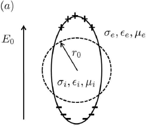
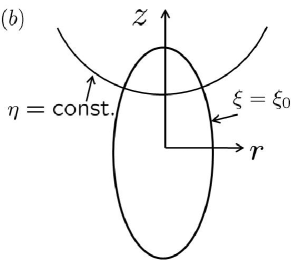
Figure 1: (a) A schematic of the problem configuration. (b) The prolate spheroidal coordinate system.

In what follows, we will solve the electrical problem first, followed by a solution of the hydrodynamic problem. An ODE for $\xi_{0}$ is obtained by applying both the stress matching and kinematic conditions.

II.1 The electrical problem

The electric potentials inside and outside the droplet obey the Laplace equation according to the Ohmic law of current conservation with uniform electrical conductivity:

$$\nabla^{2}\phi_{i}=\nabla^{2}\phi_{e}=0.$$ (5)

The matching conditions at the interface are

$$||\nabla\phi\cdot\mathbf{\bm{t}}||=0,\qquad\rm{at}\ \xi=\xi_{0},$$ (6)

$$\frac{\partial q}{\partial t}-||\sigma\nabla\phi\cdot\mathbf{\bm{n}}||=0,\qquad\rm{at}\ \xi=\xi_{0}.$$ (7)

Here $||\cdot||$ denotes a jump across an interface, and $\mathbf{\bm{t}}$ and $\mathbf{\bm{n}}$ are the unit tangential and normal interfacial vector, respectively. $q=||-\epsilon\nabla\phi\cdot\mathbf{\bm{n}}||$ is the surface charge density. Note that in Eq. (7), we have included the displacement current, $\partial q/\partial t$. This term is particularly important for fluids with very low conductivities (for example, those used in Ref. Ha and Yang (2000)) such that the interfacial charging time becomes comparable to the deformation time. However, we have ignored the effect of surface charge convection which is shown to be small by numerical simulations Feng (1999). Equation (7) can be rewritten in terms of the electric potentials,

$$\left(\frac{\epsilon_{e}}{c}\frac{\partial\phi_{e}}{\partial\xi}-\frac{\epsilon_{i}}{c}\frac{\partial\phi_{i}}{\partial\xi}\right)\frac{d\frac{c}{h_{\xi}}}{dt}-\left(\frac{\epsilon_{e}}{h_{\xi}c}\frac{\partial\phi_{e}}{\partial\xi}-\frac{\epsilon_{i}}{h_{\xi}c}\frac{\partial\phi_{i}}{\partial\xi}\right)\frac{dc}{dt}$$

$$+\left(\frac{\epsilon_{e}}{h_{\xi}}\frac{\partial^{2}\phi_{e}}{\partial\xi\partial t}-\frac{\epsilon_{i}}{h_{\xi}}\frac{\partial^{2}\phi_{i}}{\partial\xi\partial t}\right)+\frac{1}{h_{\xi}}\left(\sigma_{e}\frac{\partial\phi_{e}}{\partial\xi}-\sigma_{i}\frac{\partial\phi_{i}}{\partial\xi}\right)=0,$$

$$\qquad\qquad\qquad\qquad\qquad\qquad\qquad\qquad\qquad{\rm at}\ \xi=\xi_{0}.$$ (8)

Here $h_{\xi}$ is a metric coefficient of the prolate spheroidal coordinate system. The displacement current consists of two parts, represented by the first three terms on the LHS of the above equation. The first two terms result from a change in the droplet shape, and the third results from the charging process as if the shape remains unchanged. Here, we assume that the first term is negligible compared with the other two, and Eq. (8) can be further simplified to be

$$\epsilon_{e}\frac{\partial^{2}\phi_{e}}{\partial\xi\partial t} -\frac{\epsilon_{e}}{c}\frac{\partial\phi_{e}}{\partial\xi}\frac{dc}{dt}-\epsilon_{i}\frac{\partial^{2}\phi_{i}}{\partial\xi\partial t}+\frac{\epsilon_{i}}{c}\frac{\partial\phi_{i}}{\partial\xi}\frac{dc}{dt}$$ (9)

$$+\sigma_{e}\frac{\partial\phi_{e}}{\partial\xi}-\sigma_{i}\frac{\partial\phi_{i}}{\partial\xi}=0,\qquad{\rm at}\ \xi=\xi_{0}.$$

Indeed a consistency check a posteriori justifies the simplification. Far away from the droplet surface the electric field is uniform,

$$-\nabla\phi_{e}=E_{0}\mathbf{\bm{z}},\qquad{\rm at}\ \xi\rightarrow\infty.$$ (10)

We also require that $\phi_{i}$ remains finite at $\xi=1$. For the initial condition, we assume both the electric potential and the normal component of the displacement vector are continuous:

$$\epsilon_{e}\frac{\partial\phi_{e}}{\partial\xi}=\epsilon_{i}\frac{\partial\phi_{i}}{\partial\xi},\quad\phi_{e}=\phi_{i},\qquad{\rm at}\ \xi=\xi_{0},\;t=0.$$ (11)

Solutions for the electric potentials have been obtained previously without including the displacement current Taylor (1966); Bentenitis and Krause (2005). With its inclusion the approach is similar and the results are

$$\phi_{e}=E_{0}r_{0}\left[-\lambda\xi+\alpha Q_{1}(\xi)\right]\eta,$$ (12)

$$\phi_{i}=E_{0}r_{0}\beta\xi\eta.$$ (13)

Here, $Q_{1}(\xi)$ is a 1st-degree Legendre polynomial of the second kind. $\lambda\equiv c/r_{0}$ is the dimensionless semi-focal length. The coefficients $\alpha$ and $\beta$ are determined by the interfacial matching conditions (6) and (9) which gives

$$\alpha=\frac{\beta\xi_{0}+\lambda\xi_{0}}{Q_{1}(\xi_{0})},$$ (14)

$$\frac{\tau_{1}}{\tau_{2}}\left[\frac{Q_{1}^{{}^{\prime}}(\xi_{0})\xi_{0}}{Q_{1}(\xi_{0})}-\frac{1}{\epsilon_{r}}\right]\frac{d\beta}{d\tau}+\left[\frac{\tau_{1}}{\tau_{2}}\left(\frac{Q_{1}^{{}^{\prime}}(\xi_{0})}{Q_{1}(\xi_{0})}+\frac{Q_{1}^{{}^{\prime\prime}}(\xi_{0})Q_{1}(\xi_{0})-Q_{1}^{{}^{\prime}2}(\xi_{0})}{Q_{1}^{2}(\xi_{0})}\xi_{0}\right)\frac{d\xi_{0}}{d\tau}-\frac{\tau_{1}}{\tau_{2}}\left(\frac{Q_{1}^{{}^{\prime}}(\xi_{0})\xi_{0}}{Q_{1}(\xi_{0})\lambda}-\frac{1}{\epsilon_{r}\lambda}\right)\frac{d\lambda}{d\xi_{0}}\frac{d\xi_{0}}{d\tau}\right.$$

$$\left.+\frac{Q_{1}^{{}^{\prime}}(\xi_{0})\xi_{0}}{Q_{1}(\xi_{0})}-\frac{1}{\sigma_{r}}\right]\beta+\lambda\left[\frac{Q_{1}^{{}^{\prime}}(\xi_{0})\xi_{0}}{Q_{1}(\xi_{0})}-1\right]+\frac{\tau_{1}}{\tau_{2}}\left[\frac{Q_{1}^{{}^{\prime}}(\xi_{0})}{Q_{1}(\xi_{0})}+\frac{Q_{1}^{{}^{\prime\prime}}(\xi_{0})Q_{1}(\xi_{0})-Q_{1}^{{}^{\prime}2}(\xi_{0})}{Q_{1}^{2}(\xi_{0})}\xi_{0}\right]\lambda\frac{d\xi_{0}}{d\tau}=0,$$ (15)

$$\alpha(0)=\lambda\xi_{0}\left(\epsilon_{r}-1\right),\quad\beta(0)=\frac{\epsilon_{r}\lambda\left(Q_{1}(\xi_{0})-Q_{1}^{{}^{\prime}}(\xi_{0})\xi_{0}\right)}{\epsilon_{r}Q_{1}^{{}^{\prime}}(\xi_{0})\xi_{0}-Q_{1}(\xi_{0})}.$$ (16)

Here $\epsilon_{r}\equiv\epsilon_{e}/\epsilon_{i}$ and $\sigma_{r}\equiv\sigma_{e}/\sigma_{i}$ are the permittivity ratio and the conductivity ratio, respectively. $\tau_{1}\equiv\epsilon_{e}/\sigma_{e}$ is an electrical charging time. $\tau_{2}\equiv r_{0}\mu_{e}/\gamma$ is a characteristic flow timescale used below in the hydrodynamic problem, and $\gamma$ is the coefficient of surface tension. In the above equations, a dimensionless time $\tau\equiv t/\tau_{2}$ has been used. In general, Eq. (15) needs to be integrated together with an ODE for $\xi_{0}$ to obtain $\alpha$ and $\beta$. However, in the limit of instantaneous-charge-relaxation time, $\tau_{1}/\tau_{2}\rightarrow 0$, and Eq. (15) can be simplified to be

$$\left[\frac{Q_{1}^{{}^{\prime}}(\xi_{0})\xi_{0}}{Q_{1}(\xi_{0})}-\frac{1}{\sigma_{r}}\right]\beta+\lambda\left[\frac{Q_{1}^{{}^{\prime}}(\xi_{0})\xi_{0}}{Q_{1}(\xi_{0})}-1\right]=0.$$ (17)

This result is equivalent to a solution employing the simplified boundary condition $||\sigma\nabla\phi\cdot\mathbf{\bm{n}}||=0$ in place of Eq. (7).

The normal and tangential electrostatic stresses are given by,

$$S_{\xi\xi}=\frac{\epsilon}{2}\left(E_{\xi}^{2}-E_{\eta}^{2}\right),\qquad S_{\xi\eta}=\epsilon E_{\xi}E_{\eta},$$ (18)

where $E_{\xi}=-(\partial\phi/\partial\xi)/h_{\xi}$ and $E_{\eta}=-(\partial\phi/\partial\eta)/h_{\eta}$ are the normal and tangential electric fields, respectively. $h_{\eta}$ is a metric coefficient of the prolate spheroidal coordinate system. These stresses can be evaluated with the solutions (12) and (13), and will be used in the stress matching conditions below.

II.2 The hydrodynamic problem

In the regime of low-Reynolds-number flow, the governing equation for the hydrodynamic problem can be rewritten in terms of the stream function, $\psi$, as

$$\rm{E}^{4}\psi=0.$$ (19)

Here, the expression for the operator $\rm{E}^{2}$ can be found in Dubash and Mestel Dubash and Mestel (2007) and Bentenitis and Krause Bentenitis and Krause (2005). The stream function is related to the velocity components as

$$u=-\frac{1}{h_{\xi}h_{\theta}}\frac{\partial\psi}{\partial\xi},\qquad v=\frac{1}{h_{\eta}h_{\theta}}\frac{\partial\psi}{\partial\eta}.$$ (20)

$h_{\theta}$ is a metric coefficient of the prolate spheroidal coordinate system. At the interface, $u$ and $v$ represent the tangential and normal velocities, respectively, and they are required to be continuous

$$u_{e}=u_{i},\qquad v_{e}=v_{i},\qquad{\rm at}\ \xi=\xi_{0}.$$ (21)

In addition, we prescribe a kinematic condition relating the interfacial displacement to the normal velocity,

$$v(\xi=\xi_{0},\>\eta)=\frac{r_{0}\left(1-\xi_{0}^{-2}\right)^{-5/6}}{3\xi_{0}^{2}}\frac{\left(1-3\eta^{2}\right)}{\sqrt{\xi_{0}^{2}-\eta^{2}}}\frac{d\xi_{0}}{dt}.$$ (22)

The total force on the interface resulting from the electrical stress, the hydrodynamic stress, and the surface tension should be balanced at every point. However, this constraint is impossible to satisfy exactly within the framework of spheroidal deformation. Various authors developed reduced stress-balance conditions instead Taylor (1964); Sherwood (1988); Bentenitis and Krause (2005); Dubash and Mestel (2007). Here we follow the integrated formulae proposed by Sherwood Sherwood (1988) and Dubash and Mestel Dubash and Mestel (2007)

$$\int u\cdot\left(T_{\xi\eta}^{e}-T_{\xi\eta}^{i}+S_{\xi\eta}^{e}-S_{\xi\eta}^{i}\right)ds=0,$$ (23)

$$\int v\cdot\left(T_{\xi\xi}^{e}-T_{\xi\xi}^{i}+S_{\xi\xi}^{e}-S_{\xi\xi}^{i}-\gamma\left(\frac{1}{R_{1}}+\frac{1}{R_{2}}\right)\right)ds=0.$$ (24)

Equations (23) and (24) represent a global balance of the tangential and normal stresses, respectively derived from energy principles. Here $T$ denotes the hydrodynamic stress, $R_{1}$ and $R_{2}$ are the two principal radii of the curvature, and the integration is carried over the interface.

The general solution to (19) was proposed by Dassios et al. Dassios et al. (1994) using the method of semi-separation:

$$\psi=g_{0}(\xi) G_{0}(\eta)+g_{1}(\xi)G_{1}(\eta)$$ (25)

$$+\sum_{n=2}^{\infty}\left[g_{n}(\xi)G_{n}(\eta)+h_{n}(\xi)H_{n}(\eta)\right].$$

Here $G_{n}$ and $H_{n}$ are Gegenbauer functions of the first and second kind, respectively. $g_{n}$ and $h_{n}$ are linear combinations of $G_{n}$ and $H_{n}$. The detailed expressions for $G_{n}$, $H_{n}$, $g_{n}$, and $h_{n}$ are found in Ref. Dassios et al. (1994). Interested readers are referred to Ref. Dassios et al. (1994) for further details. After considering that the far field is quiescent, and that the velocities remain finite at $\xi=1$, the stream functions can be simplified to be

$$\psi_{e}=\sum_{n=1}^{\infty}\left[A_{2n+1}^{2n-1}H_{2n-1}(\xi)+A_{2n+1}^{2n+1}H_{2n+1}(\xi)\right.$$

$$\left.+A_{2n+1}^{2n+3}H_{2n+3}(\xi)\right]G_{2n+1}(\eta),$$ (26)

$$\psi_{i}=\sum_{n=1}^{\infty}\left[B_{2n+1}^{2n-1}G_{2n-1}(\xi)+B_{2n+1}^{2n+1}G_{2n+1}(\xi)\right.$$

$$\left.+B_{2n+1}^{2n+3}G_{2n+3}(\xi)\right]G_{2n+1}(\eta),$$ (27)

where $A$ and $B$ are unknown coefficients satisfying the relations $A_{2n+1}^{2n+3}=A_{2n+3}^{2n+1}$, $B_{2n+1}^{2n+3}=B_{2n+3}^{2n+1}$. In general, these coefficients are inter-dependent, and the full solution can be obtained only with the entire infinite series. Here we seek a truncated solution as an approximation,

$$\psi_{e}=\left[A_{3}^{1}H_{1}(\xi)+A_{3}^{3}H_{3}(\xi)\right]G_{3}(\eta),$$ (28)

$$\psi_{i}=\left[B_{3}^{3}G_{3}(\xi)+B_{3}^{5}G_{5}(\xi)\right]G_{3}(\eta).$$ (29)

Indeed, $G_{3}(\eta)$ gives a functional form in $\eta$ confirming with that in Eq. (22), which can be rewritten as

$$v(\xi=\xi_{0},\>\eta)=\frac{2c^{2}\sqrt{\xi_{0}-1}r_{0}\left(1-\xi_{0}^{-2}\right)^{-5/6}}{3\xi_{0}^{2}}\frac{G_{3}^{{}^{\prime}}(\eta)}{h_{\eta}h_{\theta}}\frac{d\xi_{0}}{dt}.$$ (30)

This agreement in part validates the spheroidal shape assumption: the shape represents the leading mode in the infinite series.

Equations (21-24) are combined to solve for the five unknown variables, namely, $A_{3}^{1}$, $A_{3}^{3}$, $B_{3}^{3}$, $B_{3}^{5}$, and $\xi_{0}$. Specifically, Eqs. (21) and (22) are first used to eliminate the $A_{3}^{1}$, $B_{3}^{3}$, $B_{3}^{5}$,

$$A_{3}^{1}=H_{3}(\xi_{0})A_{3}^{3}-M\frac{d\xi_{0}}{dt},$$ (31)

$$B_{3}^{3}=\frac{-G_{5}(\xi_{0})H_{3}^{{}^{\prime}}(\xi_{0})A_{3}^{3}+G_{5}^{{}^{\prime}}(\xi_{0})M\frac{d\xi_{0}}{dt}}{N},$$ (32)

$$B_{3}^{5}=\frac{G_{3}(\xi_{0})H_{3}^{{}^{\prime}}(\xi_{0})A_{3}^{3}-G_{3}^{{}^{\prime}}(\xi_{0})M\frac{d\xi_{0}}{dt}}{N},$$ (33)

where $M\equiv 2r_{0}^{3}/3(\xi_{0}^{3}-\xi_{0})$, and $N\equiv G_{3}(\xi_{0})G_{5}^{{}^{\prime}}(\xi_{0})-G_{3}^{{}^{\prime}}(\xi_{0})G_{5}(\xi_{0})$. Further considering Eq. (23), we can express $A_{3}^{3}$ in terms of $\xi_{0}$,

$$A_{3}^{3}=\frac{cr_{0}^{2}\epsilon_{i}E_{0}^{2}\left\{\xi_{0}\beta^{2}-\epsilon_{r}(\lambda-\alpha Q_{1}^{{}^{\prime}}(\xi_{0}))(\lambda\xi_{0}-\alpha Q_{1}(\xi_{0}))\right\}f_{11}(\xi_{0})-\mu_{i}\left\{(\mu_{r}-1)f_{12}(\xi_{0})+f_{13}(\xi_{0})\right\}M\frac{d\xi_{0}}{dt}}{-\mu_{i}\left\{\mu_{r}f_{14}(\xi_{0})+f_{15}(\xi_{0})\right\}},$$ (34)

where $\mu_{r}\equiv\mu_{e}/\mu_{i}$ is the viscosity ratio. The detailed expressions of $f_{11}(\xi_{0})-f_{15}(\xi_{0})$ are found in the Appendix. This expression is inserted into Eq. (24) to obtain the final result, an ODE governing the evolution of the $\xi_{0}$,

$$\frac{d\xi_{0}}{d\tau}=-\frac{1}{F}\left[Q_{N}f_{21}(\xi_{0})+Q_{T}\frac{\mu_{r}f_{22}(\xi_{0})+f_{23}(\xi_{0})}{\mu_{r}f_{14}(\xi_{0})+f_{15}(\xi_{0})}-f_{24}(\xi_{0})\right],$$ (35a)

$$Q_{N}=\frac{Ca_{E}}{\lambda^{2}}\left[(\lambda-\alpha Q_{1}^{{}^{\prime}}(\xi_{0}))^{2}+(\lambda-\alpha Q_{1}(\xi_{0})/\xi_{0})^{2}-2\beta^{2}/\epsilon_{r}\right],$$ (35b)

$$Q_{T}=\frac{Ca_{E}}{\lambda^{2}}\left[(\lambda-\alpha Q_{1}^{{}^{\prime}}(\xi_{0}))(\lambda-\alpha Q_{1}(\xi_{0})/\xi_{0})-\beta^{2}/\epsilon_{r}\right].$$ (35c)

The detailed expressions of $f_{21}(\xi_{0})-f_{24}(\xi_{0})$, and $F$ are also found in the Appendix. The coefficients $\alpha$ and $\beta$ are given by Eqs. (14) and (15), respectively. $Ca_{E}\equiv r_{0}\epsilon_{e}E_{0}^{2}/\gamma$ is the electric capillary number. In Eq. (35a), the three terms in the numerator on the RHS represent the contributions from the normal stress, the tangential stress, and the surface tension, respectively. At the equilibrium, the balance of the three forces determines the final shape. The leading coefficients $Q_{N}$ and $Q_{T}$ arise exclusively from the electrostatic stresses, and can be used to estimate their respective influence on deformation. In the limit of instantaneous relaxation, and by considering Eqs. (14) and (17), $Q_{N}$ and $Q_{T}$ can be simplified to be

$$Q_{N}=Ca_{E}K^{2}(\sigma_{r}^{2}+1-2\sigma_{r}^{2}/\epsilon_{r}),\\ Q_{T}=Ca_{E}K^{2}\sigma_{r}(1-\sigma_{r}/\epsilon_{r}),$$ (36)

$$K\equiv\frac{Q_{1}(\xi_{0})-\xi_{0}Q_{1}^{{}^{\prime}}(\xi_{0})}{Q_{1}(\xi_{0})-\sigma_{r}\xi_{0}Q_{1}^{{}^{\prime}}(\xi_{0})}.$$ (37)

For this case, the evolution of $\xi_{0}$ is governed by a single timescale, $\tau_{2}$. Once $\xi_{0}$ is obtained by solving the Eqs. (15) and (35a), the aspect ratio is calculated by the formula

$$\frac{a}{b}=(1-\xi_{0}^{-2})^{-\frac{1}{2}}.$$ (38)

III Comparison with previous results

In this section, we compare our model prediction extensively with results from previous work. The comparisons with theoretical/numerical results and experimental data are respectively presented in Secs. III.1 and III.2.

III.1 Comparison with previous theories and simulation

We first consider the equilibrium shape, and compare our results with those from Bentenitis and Krause Bentenitis and Krause (2005). For this case, the LHS of Eq. (35a) is simply set to zero, resulting in the so called discriminating equation,

$$Q_{N}f_{21}(\xi_{0})+Q_{T}\frac{\mu_{r}f_{22}(\xi_{0})+f_{23}(\xi_{0})}{\mu_{r}f_{14}(\xi_{0})+f_{15}(\xi_{0})}=f_{24}(\xi_{0}).$$ (39)

Here $Q_{N}$ and $Q_{T}$ are given by Eq. (36). $\xi_{0}$ is solved as a root(s) of this equation from which the equilibrium aspect ratio, $a/b$, can be obtained. Equation (39) shows that the equilibrium shape is only determined by the dimensionless parameters $Ca_{E},\>\sigma_{r},\>\epsilon_{r},$ and $\mu_{r}$. A comparison with the theoretical prediction by Bentenitis and Krause Bentenitis and Krause (2005) is shown in Fig. 2. Note that in this earlier work, the authors solved for the equilibrium shape directly without obtaining the transient solution. A good agreement is observed, although a different stress matching condition has been used by Bentenitis and Krause Bentenitis and Krause (2005) [see Eqs. (38) and (45) therein].

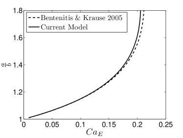
Figure 2: The equilibrium aspect ratio as a function of electric capillary number. The parameters are $\sigma_{r}=1.19\times 10^{-3}$, $\epsilon_{r}=3.24\times 10^{-1}$, and $\mu_{r}=7.33\times 10^{-2}$.

We next compare with the results from Dubash and Mestel Dubash and Mestel (2007). In this work, the authors developed a theoretical model, also with the spheroidal shape assumption, to predict the transient deformation of a conducting, inviscid droplet immersed in a viscous, nonconductive solution. This special consideration leads to significant simplifications: both the electric and hydrodynamic fields are absent within the droplet. In addition, at the equilibrium state (if one is permitted), the hydrodynamic flow outside the droplet is also quiescent, giving rise to the phenomenon termed EHS.

In our generalized framework, the solution for this case is simply achieved by setting $\sigma_{r}\rightarrow 0$ and $\mu_{r}\rightarrow\infty$ in Eqs. (35a) and (36). Note that $\sigma_{r}\rightarrow 0$ directly leads to instantaneous charge relaxation. The resulting comparisons are shown in Fig. 3 in which the aspect ratio ($a/b$) is plotted as a function of time for four different electric capillary numbers ($Ca_{E}$). For the two lower values of $Ca_{E}$, the current model has excellent agreement with both the theoretical and numerical predictions by Dubash and Mestel Dubash and Mestel (2007) [Fig. 3(a)]. For these $Ca_{E}$ values, final equilibria are achieved. As $Ca_{E}$ increases [Fig. 3(b)], the deformation becomes unstable and an equilibrium shape is no longer possible. The rapid expansion with a sharp slope at the later stage preludes droplet breakup. For these two cases, the theoretical models still agree with each other, whereas some discrepancies exist with respect to the numerical simulation, in particular for $Ca_{E}$=0.206. However, this discrepancy is in general only noticeable when the $Ca_{E}$ number is above and very close to the critical threshold of breakup ($Ca_{E}\sim$0.2044 for the case studied), due to a slight underprediction of the rate of deformation by the theoretical models. A similar trend is observed when comparing with the numerical simulation by Hirata et al. Hirata et al. (2000) (not shown). Overall, our model can serve as a good approximation to the numerical model which is considered more accurate.

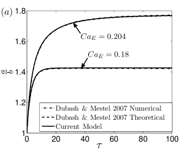
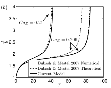
Figure 3: The deformation of a conducting droplet in a highly viscous medium. (a) $Ca_{E}=0.18$ and 0.204. (b) $Ca_{E}=0.206$ and 0.21. The dimensionless time $\tau$ is defined as $\tau=t/\tau_{2}$, where $\tau_{2}=r_{0}\mu_{e}/\gamma$.

III.2 Comparison with experimental data

The main source of experimental data comes from Ha and Yang Ha and Yang (2000). We also begin with an examination of the final aspect ratio when an equilibrium shape can be achieved. Figure 4 shows the equilibrium aspect ratio of a castor oil droplet immersed in silicone oil from Ha and Yang Ha and Yang (2000), as well as predicted by various models. The current prediction is shown as a solid line, whereas the results from first-order Taylor (1966) and second-order Ajayi (1978) theories are shown as dot-dashed and dashed lines, respectively. Following Lac and Homsy Lac and Homsy (2007), we rescale $Ca_{E}$ to best match Ajayi’s second-order correction. This rescaling is equivalent to adjusting the surface tension from $\gamma=3.3\times 10^{-3}\;{\rm N}/{\rm m}$ used by Ha and Yang Ha and Yang (2000) (which is a fitting parameter in that work) to $\gamma=4.3\times 10^{-3}\;{\rm N}/{\rm m}$. The latter value is close to the lower bound, $\gamma=4.5\times 10^{-3}\;{\rm N}/{\rm m}$, measured by Salipante and Vlahovska Salipante and Vlahovska (2010). In addition, we use $\sigma_{r}=0.03$ according to the measurements by Torza et al. Torza et al. (1971), Vizika and Saville Vizika and Saville (1992), and Salipante and Vlahovska Salipante and Vlahovska (2010), which is slightly different from the value of $\sigma_{r}=0.04$ used by Lac and Homsy Lac and Homsy (2007). The results show good agreement between the current model and the experimental data. Most importantly, our theory correctly predicts a critical $Ca_{E}$ ($\sim$0.244) for droplet breakup. In contrast, the small deformation theories can not capture this critical phenomenon.

We have also compared our theoretical prediction with the experimental data from Bentenitis and Krause Bentenitis and Krause (2005), which measured the equilibrium aspect ratio of a DGEBA droplet immersed in a PDMS solution. Since our result is in good agreement with the theoretical prediction in the same work (see Fig. 2), which in turn agrees well with the data, the comparison is not shown here for brevity.

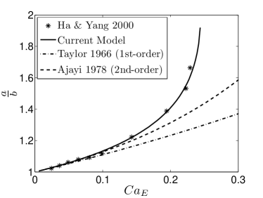
Figure 4: The prediction from current model is compared with the small deformation theories Taylor (1966); Ajayi (1978) and experimental data Ha and Yang (2000). The parameters are $\sigma_{r}=0.03$, $\epsilon_{r}=0.73$, and $\mu_{r}=1.14$.

Next, we will compare the transient solution from our model with data from Ha and Yang Ha and Yang (2000). In Fig. 5(a), the data is extracted from Fig. 3 in the latter work, which captures the deformation of a water droplet in silicone oil. The droplet is fitted with an ellipse at every instant, based on which the aspect ratio is calculated. A 10% fitting error is estimated, and is shown as error bars in Fig. 5(a) [the same approach is adopted to extract the data presented in Figs. 5(b) and 6]. The model prediction is calculated with Eqs. (35a) and (36), and with $\sigma_{r}=1\times 10^{-6}$, $\epsilon_{r}=3.55\times 10^{-2}$, $\mu_{r}=1000$, $E_{0}=3.2\;{\rm kV/cm}$, $r_{0}=0.25\;{\rm cm}$, and $\mu_{e}=0.98\;{\rm Pa\cdot s}$ all directly taken from Ha and Yang Ha and Yang (2000). For medium permittivity, we use $\epsilon_{e}=2.478\times 10^{-11}\;{\rm F}/{\rm m}$ following the measurements by Torza et al. Torza et al. (1971), Vizika and Saville Vizika and Saville (1992), and Salipante and Vlahovska Salipante and Vlahovska (2010). For surface tension, we use $\gamma=3.037\times 10^{-2}\;{\rm N}/{\rm m}$, which is consistent with the values reported by Torza et al. Torza et al. (1971) and Vizika and Saville Vizika and Saville (1992). In this case, the model is able to predict the deformation process with good quantitative accuracy. In Fig. 5(b), a similar comparison is shown for a water-ethanol droplet in silicone oil. The data is based on Fig. 4 in Ref. Ha and Yang (2000). For our calculation, $\sigma_{r}=1\times 10^{-5}$, $\epsilon_{r}=0.05$, $\mu_{r}=23.3$, $E_{0}=4.5\;{\rm kV/cm}$, $r_{0}=0.14\;{\rm cm}$, $\mu_{e}=0.98\;{\rm Pa\cdot s}$, and $\epsilon_{e}=2.478\times 10^{-11}\;{\rm F}/{\rm m}$. Because the droplet is doped with polyvinylpyrrolidone (a polymer solution), the surface tension is not directly available, and is used as a fitting parameter instead to generate the best agreement between theory and data. The resulting value is $\gamma=3.432\times 10^{-2}\;{\rm N}/{\rm m}$, 11% higher than that for water/silicone oil which is used in Fig. 5(a).

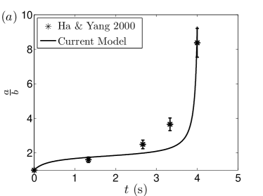
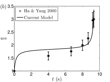
Figure 5: Comparison of transient droplet deformation. (a) A water droplet in silicone oil. The parameters are $\sigma_{r}=1\times 10^{-6}$, $\epsilon_{r}=3.55\times 10^{-2}$, $\mu_{r}=1000$, $E_{0}=3.2\;{\rm kV/cm}$, $r_{0}=0.25\;{\rm cm}$, $\mu_{e}=0.98\;{\rm Pa\cdot s}$, $\epsilon_{e}=2.478\times 10^{-11}\;{\rm F}/{\rm m}$, and $\gamma=3.037\times 10^{-2}\;{\rm N}/{\rm m}$. (b) A water-ethanol droplet in silicone oil. The parameters are $\sigma_{r}=1\times 10^{-5}$, $\epsilon_{r}=0.05$, $\mu_{r}=23.3$, $E_{0}=4.5\;{\rm kV/cm}$, $r_{0}=0.14\;{\rm cm}$, $\mu_{e}=0.98\;{\rm Pa\cdot s}$, $\epsilon_{e}=2.478\times 10^{-11}\;{\rm F}/{\rm m}$, and $\gamma=3.432\times 10^{-2}\;{\rm N}/{\rm m}$.

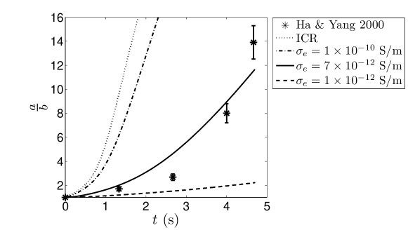
Figure 6: Droplet deformation in the limit of extremely low conductivities. The parameters are $\sigma_{r}=0.03$, $\epsilon_{r}=0.73$, $\mu_{r}=1.14$, $E_{0}=3.2\;{\rm kV/cm}$, $r_{0}=0.16\;{\rm cm}$, $\mu_{e}=0.9\;{\rm Pa\cdot s}$, $\epsilon_{e}=2.478\times 10^{-11}\;{\rm F}/{\rm m}$, and $\gamma=5\times 10^{-3}\;{\rm N}/{\rm m}$. The best agreement between the data and the theory is found for $\sigma_{e}=7\times 10^{-12}\;{\rm S/m}$. For reference, the dotted line shows the calculation according to the instantaneous-charge-relaxation (ICR) model.

In contrast to the regime of instantaneous charge relaxation examined in Fig. 5, Fig. 6 represents droplet deformation in the finite-charging-time regime. The data is extracted from Fig. 7 in Ref. Ha and Yang (2000). For this case, the droplet is made of castor oil, and is immersed in silicone oil. The extremely low conductivities of these media lead to a charging time ($\sim$seconds) comparable to the deformation time, and the full model, Eqs. (35a)-(35c), has to be used. For our calculation, $\sigma_{r}=0.03$, $\epsilon_{r}=0.73$, $\mu_{r}=1.14$, $E_{0}=3.2\;{\rm kV/cm}$, $r_{0}=0.16\;{\rm cm}$, $\mu_{e}=0.9\;{\rm Pa\cdot s}$, $\epsilon_{e}=2.478\times 10^{-11}\;{\rm F}/{\rm m}$, and $\gamma=5\times 10^{-3}\;{\rm N}/{\rm m}$. Note that the values for the surface tension and the conductivity ratio follow the measurements by Torza et al. Torza et al. (1971), Vizika and Saville Vizika and Saville (1992), and Salipante and Vlahovska Salipante and Vlahovska (2010) which are believed to be more accurate than the original values of $\sigma_{r}=0.1$ and $\gamma=3.3\times 10^{-3}\;{\rm N}/{\rm m}$ given by Ha and Yang Ha and Yang (2000). In addition, the actual conductivity of silicone oil varies from $10^{-10}\;{\rm S/m}$ to $10^{-13}\;{\rm S/m}$ in the literature Park et al. (2009); Salipante and Vlahovska (2010); Kim et al. (2011). In Fig. 6, we show the calculation with three representative values within this range, namely, $\sigma_{e}=1\times 10^{-10}$, $7\times 10^{-12}$, and $1\times 10^{-12}\;{\rm S/m}$. The best agreement is found for $\sigma_{e}=7\times 10^{-12}\;{\rm S/m}$. For comparison, the calculation according to the instantaneous-charge-relaxation model [Eqs. (35a) and (36)] is also shown, and is denoted by ICR. This simplified model clearly overpredicts deformation by a significant degree.

In general, our model agrees well with experimental data in both steady and transient states, and for a large parametric range. These comparisons provide a strong validation for our model.

IV The effects of stresses on deformation

In this section, we demonstrate the utility of our theoretical results by analyzing in-depth the governing equation. For simplicity, we focus on the regime of instantaneous relaxation, where $Q_{N}$ and $Q_{T}$ are given by Eq. (36). A main contribution of the current work is that Eq. (35a) clearly separates the effects by different forces. In the numerator of the RHS, the three terms represent respectively the effects of the normal stresses (both electrical and hydrodynamic), the tangential stresses (both electrical and hydrodynamic), and the surface tension. Furthermore, all the functions in this equation are positive ($f_{14}$, $f_{15}$, $f_{21}-f_{24}$, $F$), such that the signs of $Q_{N}$ and $Q_{T}$ completely determine whether the normal and tangential stresses would promote or suppress deformation. Due to the inverse relationship between $\xi_{0}$ and the aspect ratio, $a/b$ [see Eq. (38)], a positive $Q_{N}$ or $Q_{T}$ indicates a positive contribution. Evidently, surface tension always resists deformation. Because $Q_{N}$ and $Q_{T}$ depend exclusively on the electrical properties in a simple manner [see Eq. (36)], their influences can be conveniently analyzed using a phase diagram shown in Fig. 7. The dashed and dotted lines correspond to $Q_{N}=0$ and $Q_{T}=0$, respectively. These lines separate the phase space into three regimes, where $N$ and $T$ denote the normal and tangential stresses, and the superscripts ${}^{\prime}+^{\prime}$ and ${}^{\prime}-^{\prime}$ denote a positive or negative contribution to deformation, respectively. In addition, the solid line is obtained by solving for the root of Taylor’s discriminating function Taylor (1966), which separates the prolate (denoted by ${}^{\prime}Pr^{\prime}$) and oblate (denoted by ${}^{\prime}Ob^{\prime}$) regimes [this line can be equivalently obtained by looking for the steady-state solution of $a/b=1$ from Eq. (39)].

Figure 7 can be used to shed light on the physical processes governing deformation. First, the line for $Q_{T}=0$ separates the $T^{+}$ and $T^{-}$ regimes, which corroborates with the previous results Taylor (1966); Lac and Homsy (2007). On this dividing line, the velocity field becomes zero, so does the tangential electrical stress. In Ref. Lac and Homsy (2007), the viscosity ratio has opposite effects on deformation in the $T^{+}$ and $T^{-}$ regimes. This behavior is clearly explained by Eq. (35a). Second, there is a small region within the oblate regime, namely, the area between the solid and dashed lines where $Q_{N}$ is positive. This suggests that the normal stress still tends to stretch the droplet along the direction of the applied field. However, because $Q_{T}$ is negative, the tangential stresses overcome the normal stresses, and stretch the droplet into an oblate shape. This new insight is not available from previous analysis or simulations.

Third, in the prolate regime where $Q_{N}$ is always positive, the sign of $Q_{T}$ leads to different deformation behavior. Figure 8 shows the equilibrium aspect ratio as a function of $Ca_{E}$ for three specific cases. Note that the new variable

$$D=\frac{a-b}{a+b}.$$ (40)

In this new definition, $D=0$ corresponds to $a/b=1$, and $D=1$ corresponds to $a/b\rightarrow\infty$. For all three cases, $\epsilon_{r}=10$ and $\mu_{r}=1$. For $\sigma_{r}=0.05$, $Q_{T}>0$. We observe hysteresis, and $D$ approaches 1 rapidly in the upper brunch. The cases of $\sigma_{r}=1$ and $\sigma_{r}=30$ correspond to $Q_{T}=0$ and $Q_{T}<0$, respectively. In general, as $Q_{T}$ decreases, the deformation becomes weaker for comparable $Ca_{E}$ values. Most interestingly, for $\sigma_{r}=30$ ($Q_{T}<0$), $D$ converges to a value less than 1 in the limit of $Ca_{E}\rightarrow\infty$. This means that even for the very large applied electric field strength, a finite equilibrium aspect ratio can be achieved. We emphasize this scenario is only possible in the $T^{-}$ regime. For large $E_{0}$ values, corresponding to large $Ca_{E}$, the resistive effect from surface tension is negligible, and the only way to obtain a finite equilibrium aspect ratio is therefore by balancing the normal and tangential stresses. Since $Q_{N}$ is positive, $Q_{T}$ has to be negative.

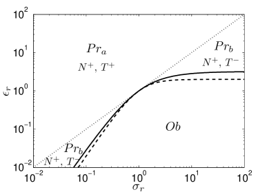
Figure 7: Phase diagram for droplet deformation. Here the dotted line is calculated by satisfying $Q_{T}=0$. The solid line is calculated by solving for the root of Taylor’s discriminating function. The dashed line represents $Q_{N}=0$. $Pr$ and $Ob$ denote prolate and oblate deformation, respectively. $N$ and $T$ denote the effect of normal and tangential stresses, respectively, and a ${}^{\prime}+^{\prime}$ or ${}^{\prime}-^{\prime}$ sign denotes facilitating or suppressing, respectively.

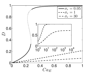
Figure 8: The behavior of equilibrium droplet deformation in different regimes. For $\sigma_{r}=0.05$, $Q_{T}>0$; $\sigma_{r}=1$, $Q_{T}=0$; $\sigma_{r}=30$, $Q_{T}<0$. As $Ca_{E}\rightarrow\infty$, an equilibrium shape is only possible in the $T^{-}$ regime. Other parameters are $\epsilon_{r}=10$ and $\mu_{r}=1$.

V Conclusions

In conclusion, we have developed a transient analysis to quantify droplet deformation under DC electric fields. The full Taylor-Melcher leaky dielectric model is employed where the charge relaxation time is considered finite. In this framework, instantaneous charge relaxation is treated as a special limiting case. The droplet is assumed to be spheroidal in shape for all times. The main result is an ODE governing the evolution of the droplet aspect ratio. The model is validated by extensively comparing predicted deformation with both previous theoretical and numerical studies, and with experimental data. In particular, the experimental results by Ha and Yang Ha and Yang (2000), which were obtained with extremely low medium conductivities are well captured by the simulation with the finite-time charge-relaxation model. The model is used to analyze the effects of parameters and stresses on the deformation characteristics. The results demonstrate clearly that in different regimes according to the sign of $Q_{T}$, the stresses contribute qualitatively differently to deformation. Last but not least, this work lays the foundation for the study of a more complex problem, namely, vesicle electrodeformation and relaxation. This problem is the pursuit of our future work.

Appendix A Appendixes

The functions $f_{11}(\xi_{0})-f_{15}(\xi_{0})$ in Eq. (34) are given in the following expressions:

$$f_{11}(\xi_{0})=\int\frac{G_{3}(\eta)\eta}{(\xi_{0}^{2}-\eta^{2})}d\eta,$$ (41)

$$f_{12}(\xi_{0})=\frac{1}{\xi_{0}^{2}-1}\left\{\int\frac{G_{3}(\eta)\eta}{(\xi_{0}^{2}-\eta^{2})}\left(\frac{(1-3\eta^{2})}{(\xi_{0}^{2}-\eta^{2})}-3\right)d\eta\right\},$$ (42)

$$f_{13}(\xi_{0})=\frac{G_{3}^{{}^{\prime\prime}}(\xi_{0})G_{5}^{{}^{\prime}}(\xi_{0})-G_{3}^{{}^{\prime}}(\xi_{0})G_{5}^{{}^{\prime\prime}}(\xi_{0})}{2N}\cdot f_{11}(\xi_{0}),$$ (43)

$$f_{14}(\xi_{0})=-\xi_{0}H_{3}^{{}^{\prime}}(\xi_{0})\int\frac{G_{3}(\eta)\eta}{(\xi_{0}^{2}-\eta^{2})^{2}}d\eta+\frac{1}{2}H_{3}^{{}^{\prime\prime}}(\xi_{0})f_{11}(\xi_{0}),$$ (44)

$$f_{15}(\xi_{0})=-\frac{H_{3}^{{}^{\prime}}(\xi_{0})\left[G_{3}(\xi_{0})G_{5}^{{}^{\prime\prime}}(\xi_{0})-G_{3}^{{}^{\prime\prime}}(\xi_{0})G_{5}(\xi_{0})\right]}{2N}f_{11}(\xi_{0})+\xi_{0}H_{3}^{{}^{\prime}}(\xi_{0})\int\frac{G_{3}(\eta)\eta}{(\xi_{0}^{2}-\eta^{2})^{2}}d\eta.$$ (45)

The functions $f_{21}(\xi_{0})-f_{24}(\xi_{0})$ and $F$ in Eq. (35a) are given in the following expressions:

$$f_{21}(\xi_{0})=\frac{1}{2}\xi_{0}^{2}\int\frac{(\eta^{2}-1)(3\eta^{2}-1)}{(\xi_{0}^{2}-\eta^{2})}d\eta,$$ (46)

$$f_{22}(\xi_{0})=\xi_{0}f_{11}(\xi_{0})\left[-H_{3}^{{}^{\prime}}(\xi_{0})\int\frac{(1-3\eta^{2})(\xi_{0}^{2}-3\xi_{0}^{2}\eta^{2}+2\eta^{4})}{(\xi_{0}^{2}-\eta^{2})^{2}}d\eta+3\xi_{0}H_{3}(\xi_{0})\int\frac{1-3\eta^{2}}{(\xi_{0}^{2}-\eta^{2})}d\eta\right],$$ (47)

$$f_{23}(\xi_{0})=\xi_{0}f_{11}(\xi_{0})\left[-\frac{49(1-3\xi_{0}^{2})G_{3}(\xi_{0})H_{3}^{{}^{\prime}}(\xi_{0})}{30N}+H_{3}^{{}^{\prime}}(\xi_{0})\int\frac{(1-3\eta^{2})(\xi_{0}^{2}-3\xi_{0}^{2}\eta^{2}+2\eta^{4})}{(\xi_{0}^{2}-\eta^{2})^{2}}d\eta\right],$$ (48)

$$f_{24}(\xi_{0})=\xi_{0}^{3}(1-\xi_{0}^{-2})^{\frac{5}{6}}\int\frac{3\eta^{2}-1}{(\xi_{0}^{2}-\eta^{2})^{\frac{3}{2}}}d\eta+\xi_{0}(1-\xi_{0}^{-2})^{-\frac{1}{6}}\int\frac{3\eta^{2}-1}{\sqrt{\xi_{0}^{2}-\eta^{2}}}d\eta,$$ (49)

$$F=-\frac{2}{3}\left(f_{25}(\xi_{0})+f_{26}(\xi_{0})/\mu_{r}\right),$$ (50)

where

$$f_{25}(\xi_{0})=-\frac{f_{22}(\xi_{0})}{\xi_{0}f_{11}(\xi_{0})}\frac{(\mu_{r}-1)f_{12}(\xi_{0})+f_{13}(\xi_{0})}{\mu_{r}f_{14}(\xi_{0})+f_{15}(\xi_{0})}-3\xi_{0}\int\frac{3\eta^{2}-1}{(\xi_{0}^{2}-\eta^{2})}d\eta-\frac{\xi_{0}}{\xi_{0}^{2}-1}\int\frac{(2\xi_{0}^{2}-\eta^{2}-1)(1-3\eta^{2})^{2}}{(\xi_{0}^{2}-\eta^{2})^{2}}d\eta,$$ (51)

$$f_{26}(\xi_{0})=-\frac{f_{23}(\xi_{0})}{\xi_{0}f_{11}(\xi_{0})}\frac{(\mu_{r}-1)f_{12}(\xi_{0})+f_{13}(\xi_{0})}{\mu_{r}f_{14}(\xi_{0})+f_{15}(\xi_{0})}-\frac{49(1-3\xi_{0}^{2})G_{3}^{{}^{\prime}}(\xi_{0})}{30N}+\frac{\xi_{0}}{\xi_{0}^{2}-1}\int\frac{(2\xi_{0}^{2}-\eta^{2}-1)(1-3\eta^{2})^{2}}{(\xi_{0}^{2}-\eta^{2})^{2}}d\eta.$$ (52)

References

- Wu and Clark (2008) Y. Wu and R. L. Clark, J. Biomater. Sci. Polymer Edn 19, 573 (2008).
- Kanazawa et al. (2008) S. Kanazawa, Y. Takahashi, and Y. Nomoto, IEEE Trans. Ind. Appl. 44, 1084 (2008).
- Basaran (2002) O. A. Basaran, AIChE J. 48, 1842 (2002).
- Allan and Mason (1962) R. S. Allan and S. G. Mason, Proc. R. Soc. Lond. A 267, 45 (1962).
- Taylor (1964) G. I. Taylor, Proc. R. Soc. Lond. A 280, 383 (1964).
- Miksis (1981) M. J. Miksis, Phys. Fluids 24, 1967 (1981).
- Sherwood (1988) J. D. Sherwood, J. Fluid Mech. 188, 133 (1988).
- Ha and Yang (2000) J.-W. Ha and S.-M. Yang, J. Fluid Mech. 405, 131 (2000).
- Dubash and Mestel (2007) N. Dubash and A. J. Mestel, J. Fluid Mech. 581, 469 (2007).
- Taylor (1966) G. I. Taylor, Proc. R. Soc. Lond. A 291, 159 (1966).
- Torza et al. (1971) S. Torza, R. G. Cox, and S. G. Mason, Phil. Trans. R. Soc. Lond. A 269, 295 (1971).
- Ajayi (1978) O. O. Ajayi, Proc. R. Soc. Lond. A 364, 499 (1978).
- Vizika and Saville (1992) O. Vizika and D. A. Saville, J. Fluid Mech. 239, 1 (1992).
- Feng and Scott (1996) J. Q. Feng and T. C. Scott, J. Fluid Mech. 311, 289 (1996).
- Baygents et al. (1998) J. C. Baygents, N. J. Rivette, and H. A. Stone, J. Fluid Mech. 368, 359 (1998).
- Feng (1999) J. Q. Feng, Proc. R. Soc. Lond. A 455, 2245 (1999).
- Hirata et al. (2000) T. Hirata, T. Kikuchi, T. Tsukada, and M. Hozawa, J. Chem. Engng Japan 33, 160 (2000).
- Bentenitis and Krause (2005) N. Bentenitis and S. Krause, Langmuir 21, 6194 (2005).
- Sato et al. (2006) H. Sato, N. Kaji, T. Mochizuki, and Y. H. Mori, Phys. Fluids 18, 127101 (2006).
- Lac and Homsy (2007) E. Lac and G. M. Homsy, J. Fluid Mech. 590, 239 (2007).
- Melcher and Taylor (1969) J. R. Melcher and G. I. Taylor, Annu. Rev. Fluid Mech. 1, 111 (1969).
- Saville (1997) D. A. Saville, Annu. Rev. Fluid Mech. 29, 27 (1997).
- Zhang et al. (2011) J. Zhang, J. D. Zahn, and H. Lin, J. Fluid Mech. 681, 293 (2011).
- Dassios et al. (1994) G. Dassios, M. Hadjinicolaou, and A. C. Payatakes, Q. Appl. Math. 52, 157 (1994).
- Salipante and Vlahovska (2010) P. F. Salipante and P. M. Vlahovska, Phys. Fluids 22, 112110 (2010).
- Park et al. (2009) J. K. Park, J. C. Ryu, W. K. Kim, and K. H. Kang, J. Phys. Chem. B 113, 12271 (2009).
- Kim et al. (2011) P. Kim, C. Duprat, S. S. H. Tsai, and H. A. Stone, Phys. Rev. Lett. 107, 034502 (2011).